Sun-Induced Chlorophyll Fluorescence III: Benchmarking Retrieval Methods and Sensor Characteristics for Proximal Sensing

 , , ,
, , ,  ,
,  , , , and
Abstract
:
1. Introduction
2. Background on Frequently Used SIF Retrieval Methods for Proximal Sensing
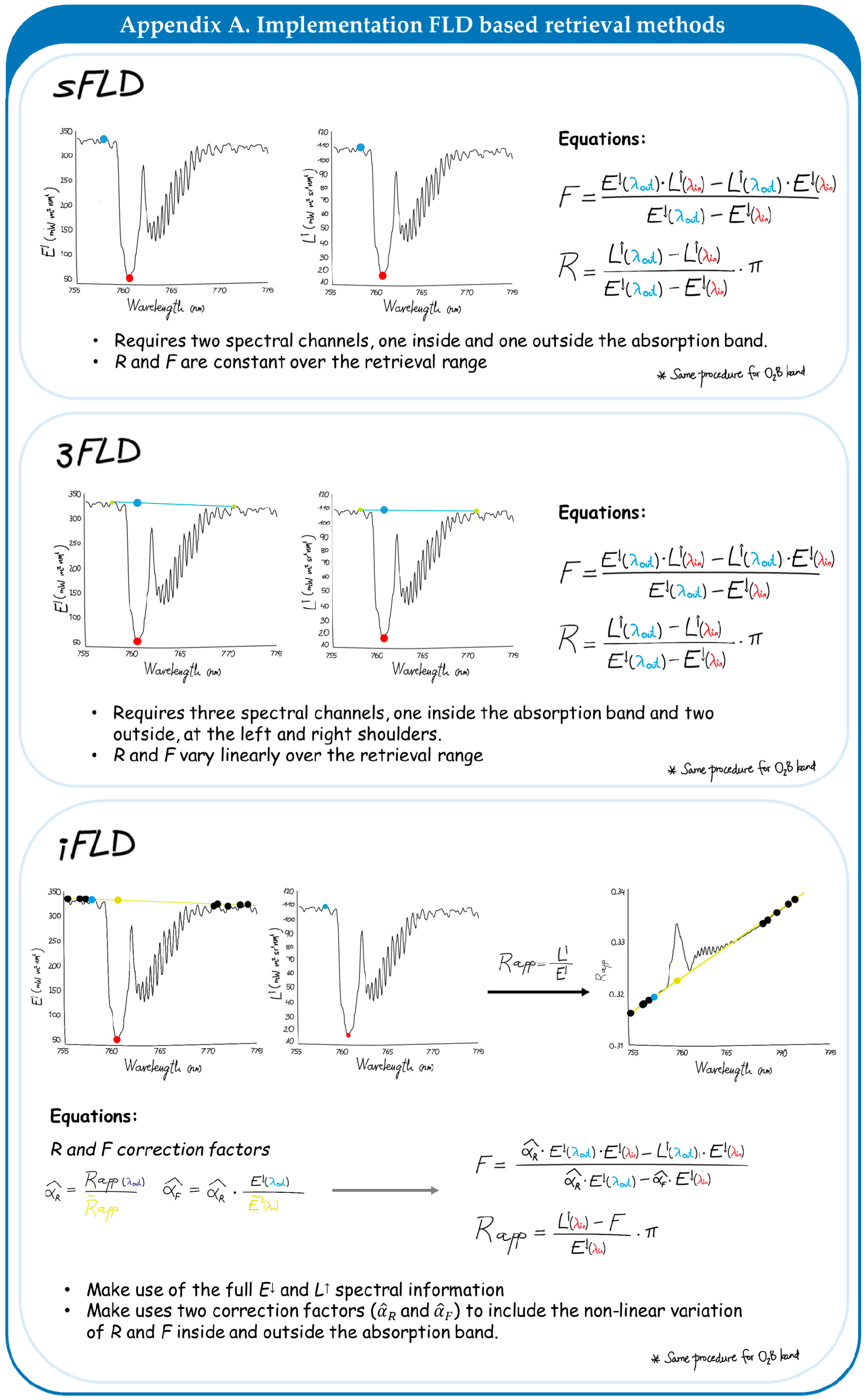
2.1. FLD-Based SIF Retrieval Methods
2.1.1. sFLD
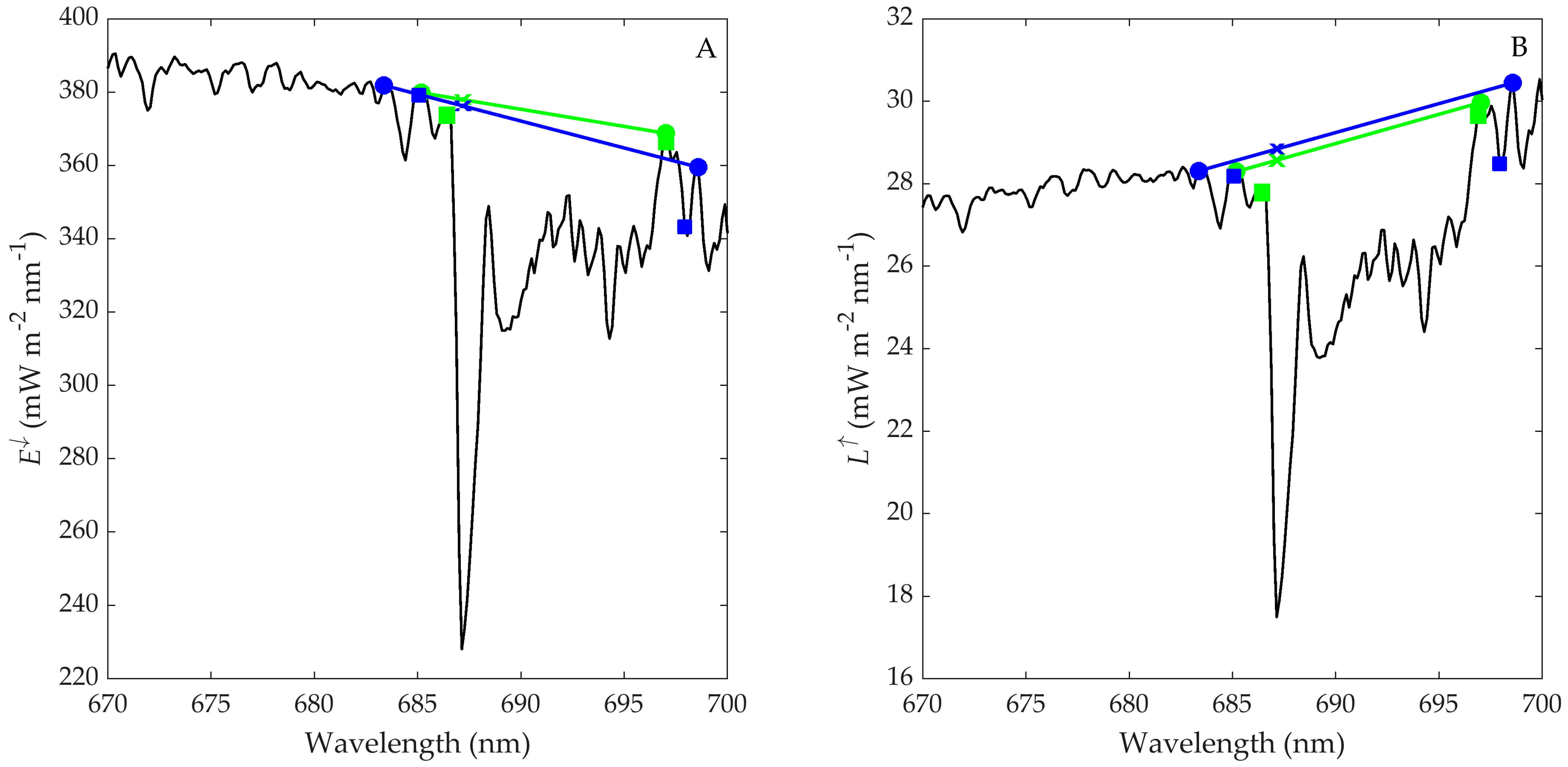
2.1.2. 3FLD
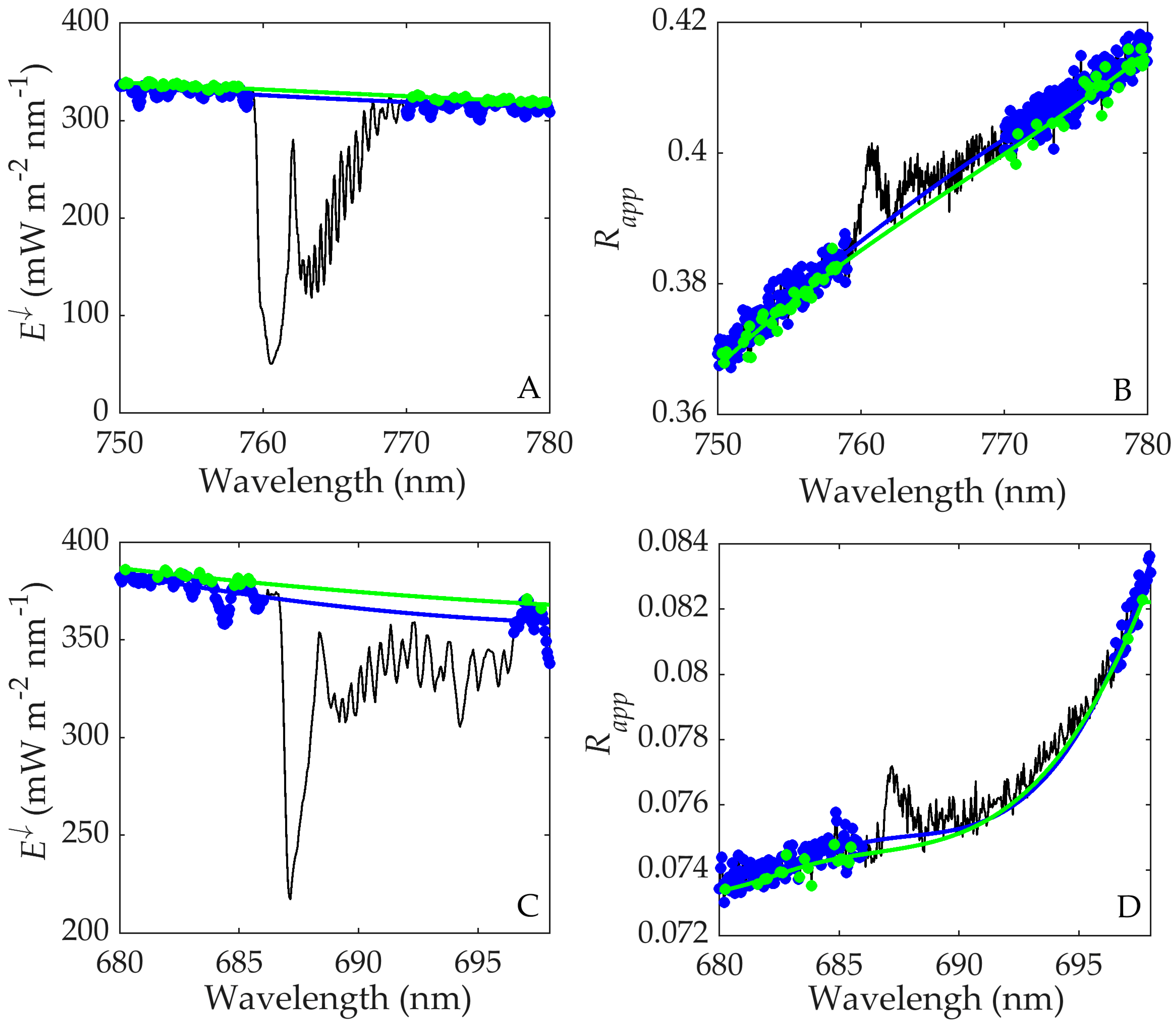
2.1.3. iFLD
2.1.4. Implementation of the FLD-Based Methods
2.2. Spectral Fitting Method-Based SIF Retrieval
2.2.1. Background of the Spectral Fitting Method
2.2.2. SFM Retrieval Method Implementation
3. Assessment of SIF Retrieval Uncertainties-Sensitivity Analysis
4. Results and Discussion
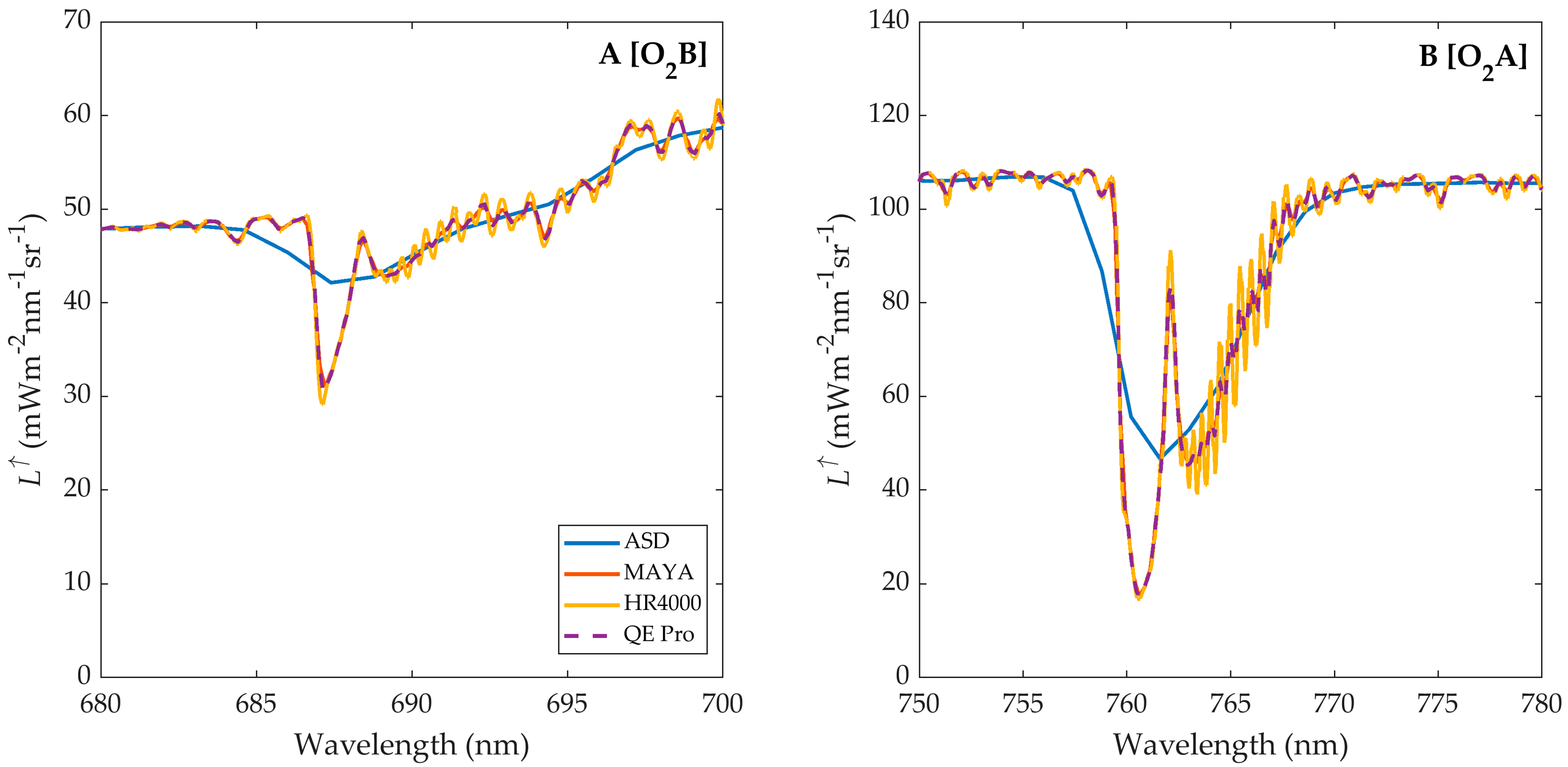
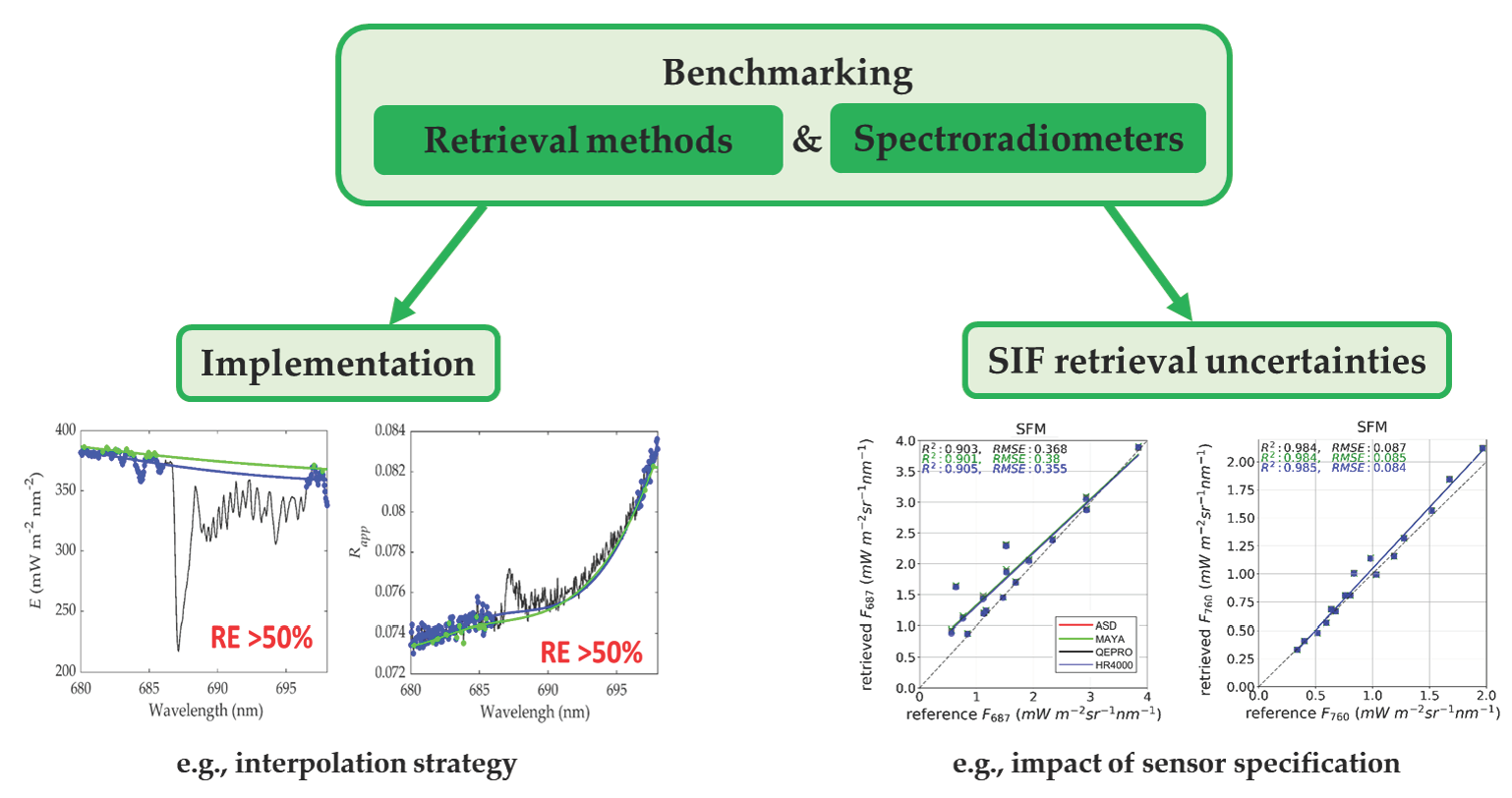
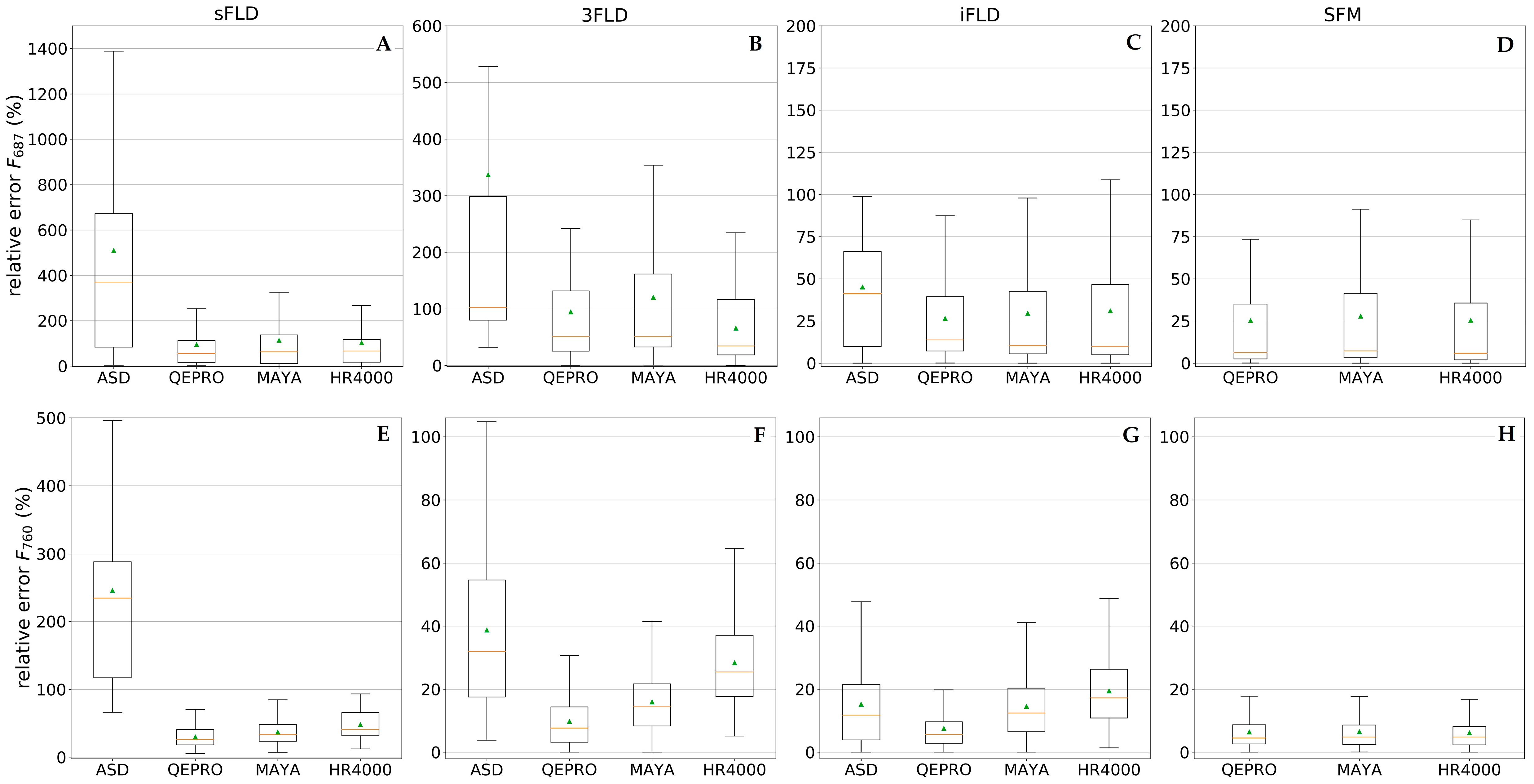
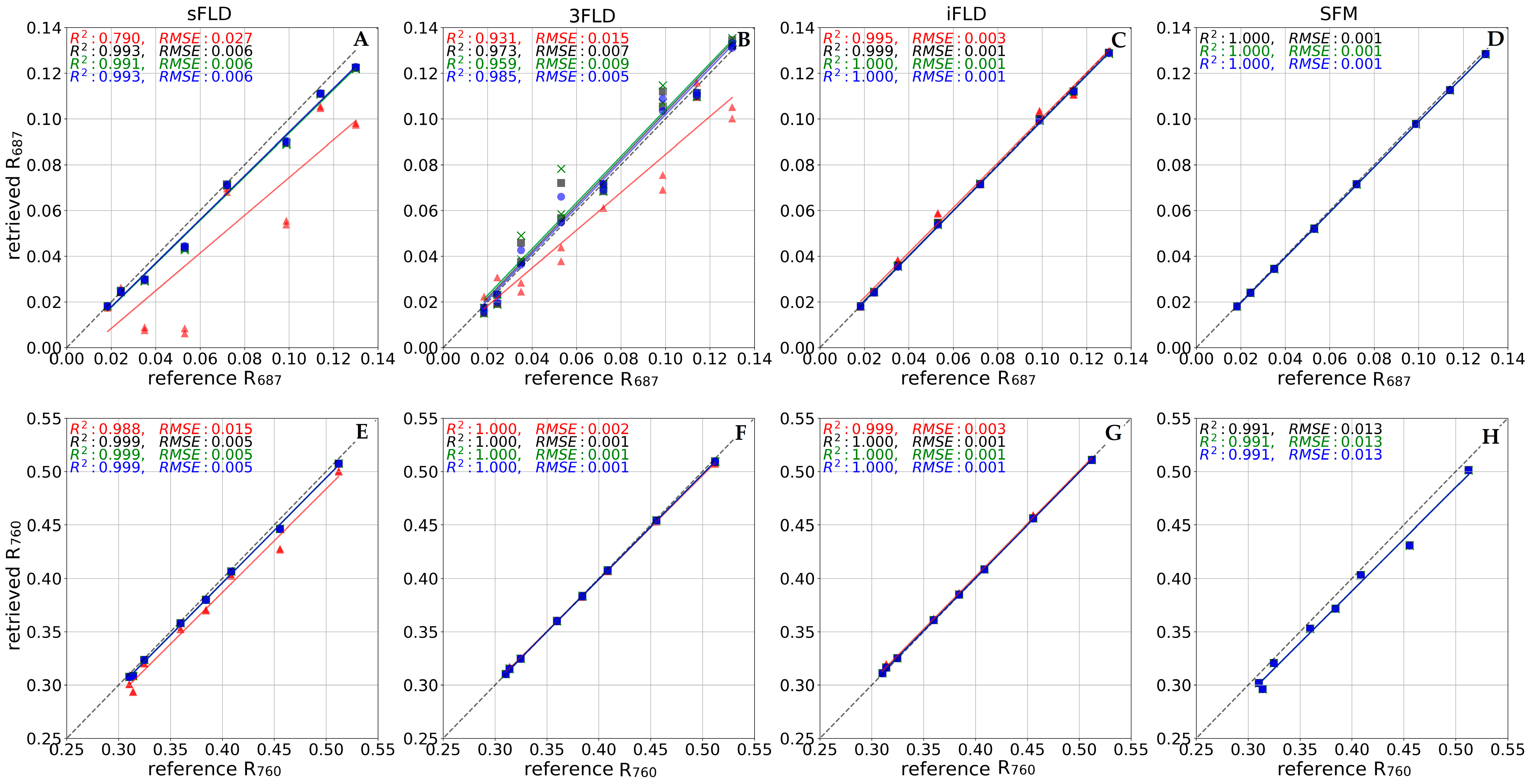
4.1. Impact of Sensor Specification on SIF Retrieval Methods
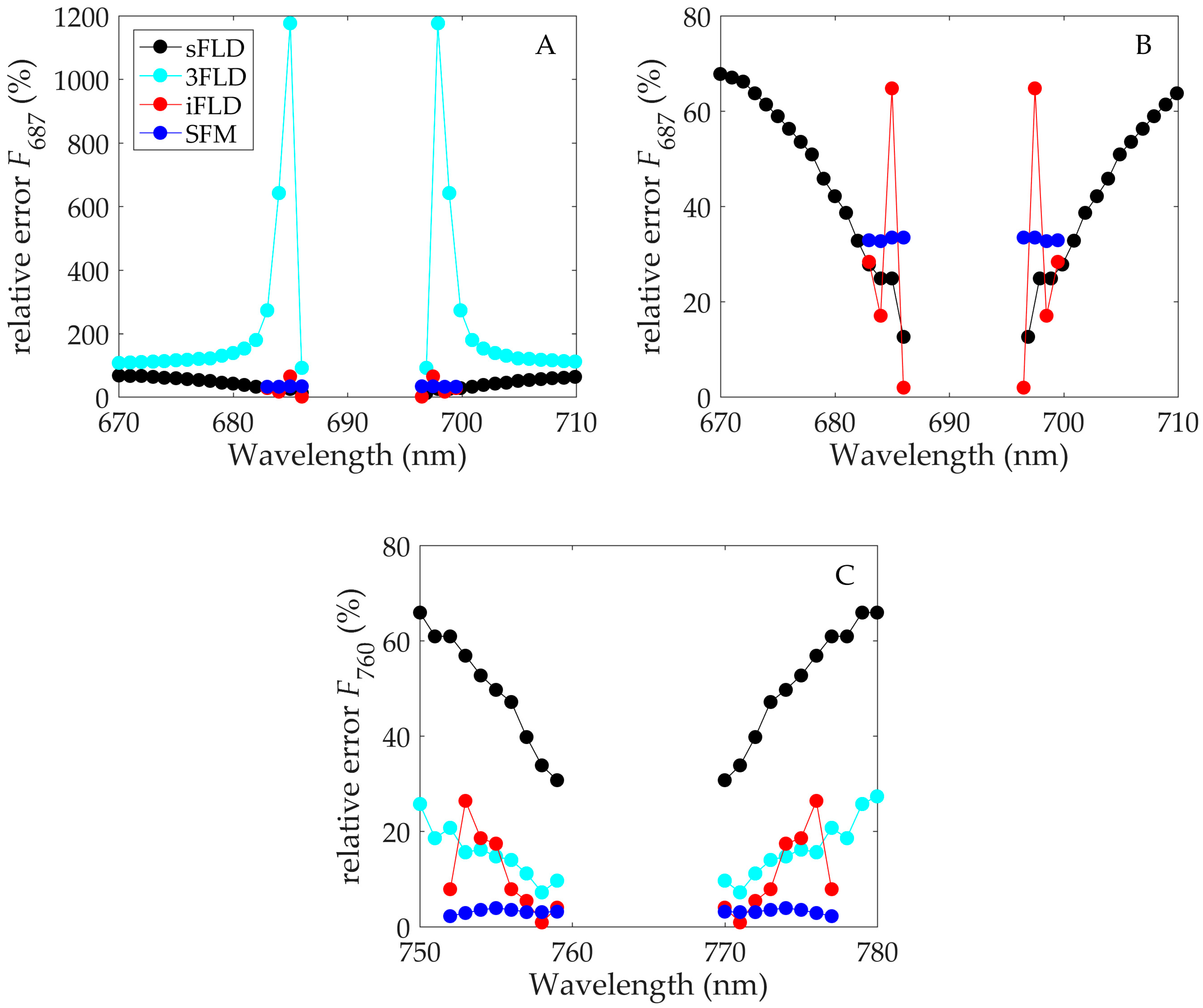
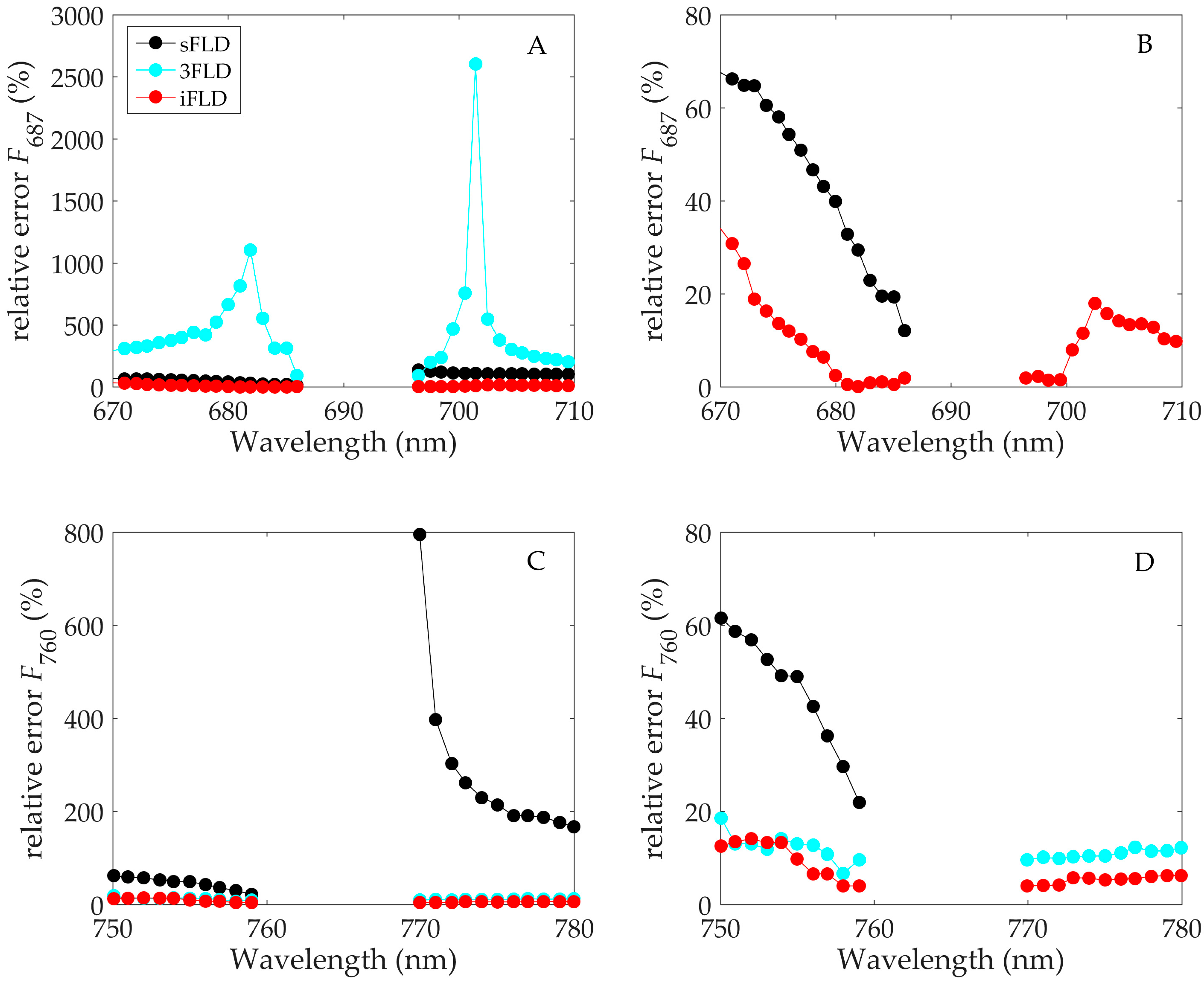
4.2. Uncertainties Caused by the Setup of Retrieval Methods
- (1)
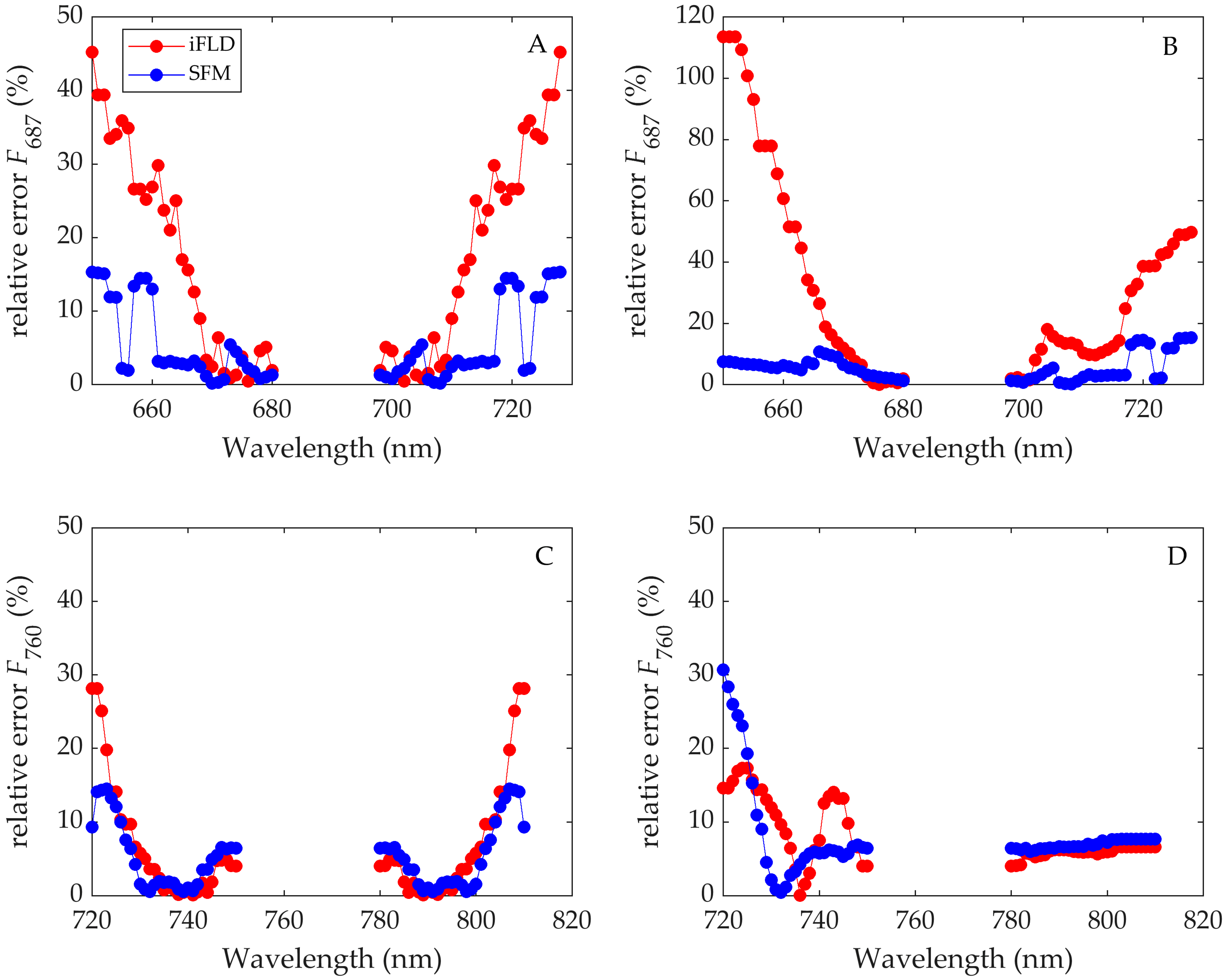
- Definition of the wavelength interval affected by O2B and O2A absorption according to instrumental spectral characteristics (FLD-based and SFM methods).
- (2)
- Selection of wavelengths at the shoulder and inside the absorption feature (FLD-based methods).
- (3)
- Interpolation strategy to estimate F and R at wavelengths affected by O2 absorption (FLD-based and SFM method).
- (4)
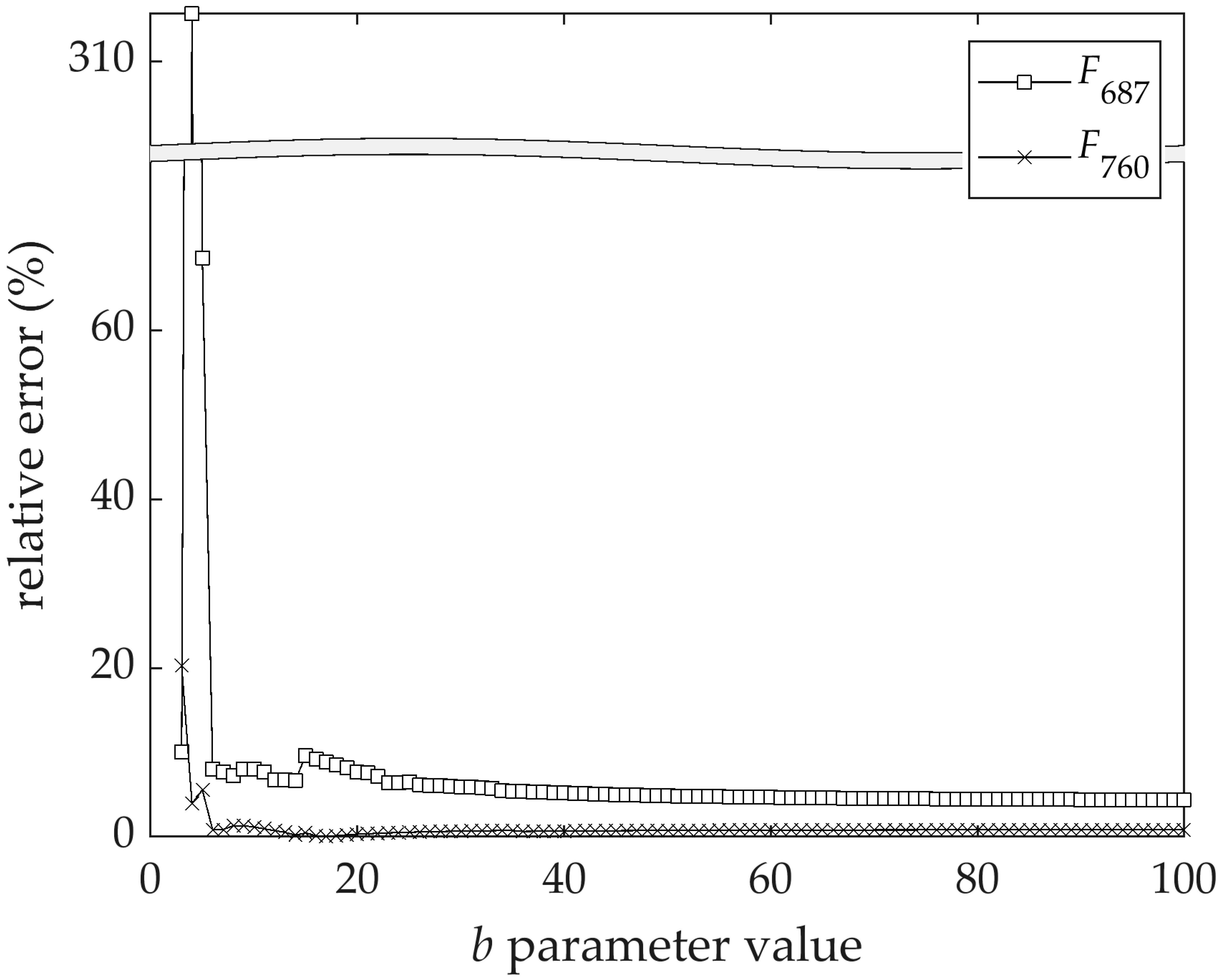
- Definition of the b parameter (SFM method).
5. Conclusions
Author Contributions
Funding
Acknowledgments
Conflicts of Interest
Abbreviations
| Description | Acronym | Units |
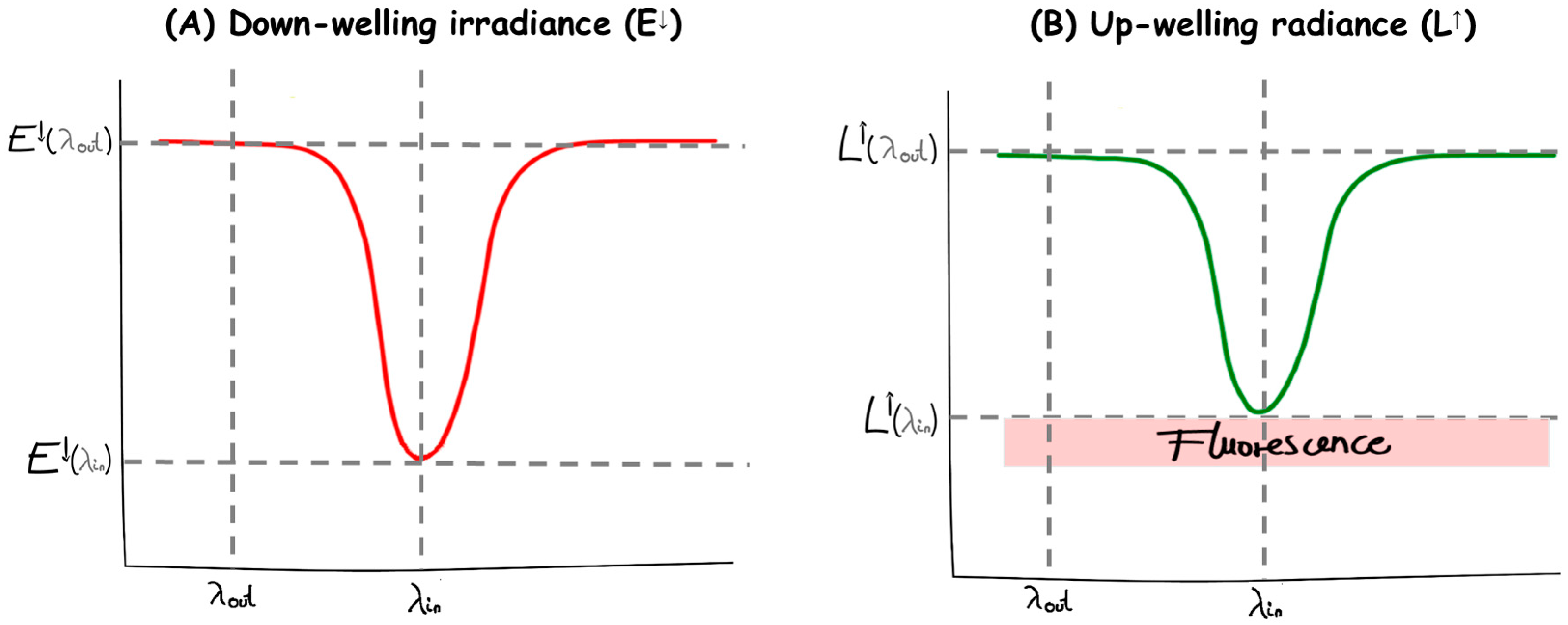
| Up-welling radiance Spectral canopy-leaving radiance in the observation direction, including both the reflected component (LR) and the emitted component (F). It is defined as the radiant flux emitted, reflected, transmitted, or received by a surface, per unit projected area per unit solid angle per wavelength. It is a directional quantity. | L↑, Lout | [mWm−2sr−1nm−1] |
| Reflected radiance Spectral reflected radiance in the observation direction. | LR, Lrefl | |
| Down-welling irradiance Spectral incoming irradiance integrated over the entire hemisphere. It is defined as the radiant flux received by a surface per unit area per wavelength. It is not a directional quantity. | E↓, Ein | [mWm−2nm−1] |
| Reflectance factor The spectrally resolved ratio of the amount of radiation reflected by a surface to the amount of radiation incident on the surface, for a specific observation geometry. | R | [-] |
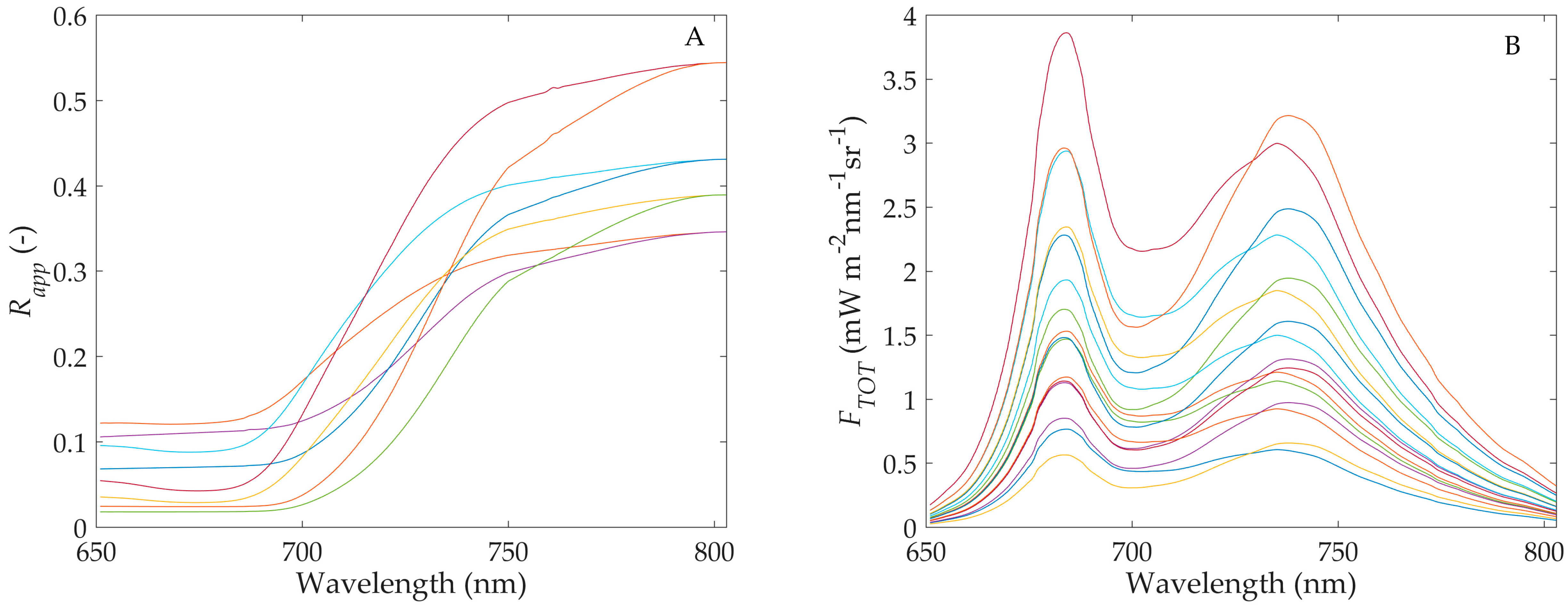
| Apparent reflectance factor The spectrally resolved ratio of the amount of radiation reflected and emitted by a surface (i.e., including fluorescence) to the amount of radiation incident on the surface, for a specific observation geometry. | Rapp, R* | [-] |
| Spectroradiometer A device designed to measure spectrally resolved radiance/irradiance over a defined region of the electromagnetic spectrum. | ||
| Spectral resolution Describes the ability of a spectrometer to define fine wavelength intervals. The finer the spectral resolution, the narrower the wavelength range for a particular band. | SR | [nm, µm] |
| Spectral sampling interval Distance between the central wavelength of two consecutive spectral bands. | SSI | [nm, µm] |
| Full width half maximum Width, at half of its maximum amplitude, of a function describing the spectral response of a spectral band. | FWHM | [nm, µm] |
| Signal-to-noise ratio Ratio between the power of a signal to the power of instrument noise, measured for the same spectral band. | SNR | [-, dB] |
| Spectral band/Spectral line A certain region of the electromagnetic spectrum sampled with an instrument, defined by its FWHM and central wavelength. Resulting from the emission, reflection, absorption, or transmission of light in a narrow frequency range. | ||
| Spectral window A certain region of the electromagnetic spectrum, defined inside a minimum and maximum wavelength range. | ||
| Multispectral Involving a limited number (e.g., 3–20) distinct regions of the electromagnetic spectrum with a relatively coarse spectral resolution (e.g., 10–50 nm FWHM). | ||
| Hyperspectral Involving a large number of nearly contiguous, partially overlapping spectral regions (e.g., 100–1000) with a relatively high spectral resolution (e.g., 0.01–3 nm FWHM). | ||
| Radiative transfer model A set of equations describing the interaction between the electromagnetic radiation and a certain medium (e.g., atmosphere, vegetation). | RTM | |
| Solar and Earth atmosphere absorption features Spectral regions in which the incoming radiance at ground level is strongly reduced due to absorption by specific chemical compounds. | ||
| Absorption features due to absorption in the solar atmosphere (i.e., solar Fraunhofer lines). These spectral regions appear “dark” also at top of Earth atmosphere. | e.g., Hα, FeI, KI | |
| Absorption features due to absorption in the Earth atmosphere (i.e., telluric). | e.g., O2A, O2B, H2O | |
| Shoulder of the absorption features The closest spectral region to an absorption feature that is not influenced by the absorption, usually referred to as left shoulder (towards shorter wavelengths) or right shoulder (towards longer wavelengths). | ||
| Sun-induced fluorescence | SIF | |
| Spectral fluorescence radiance in the observation direction | F | [mWm−2sr−1nm−1] |
| Integral of the F spectrum over the full retrieval range (e.g., 670–780 nm, 650–850 nm) | FINT | [mWm−2sr−1] |
| F emitted in the red region of the spectrum at a specific wavelength (not an integrated value), depending on the retrieval method used. | FR | [mWm−2sr−1nm−1] |
| F emitted in the far-red region of the spectrum at a specific wavelength (not an integrated value), depending on the retrieval method used. | FFR | [mWm−2sr−1nm−1] |
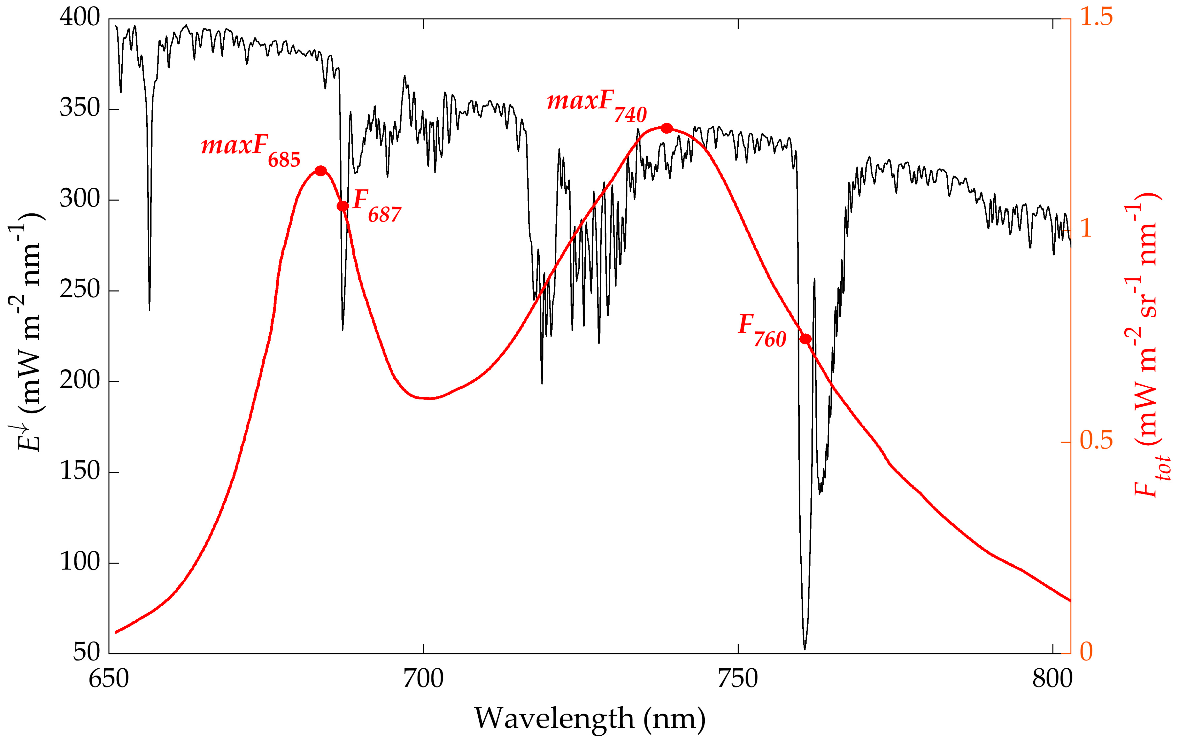
| Maximum value of F in the red region | maxFR | [mWm−2sr−1nm−1] |
| Maximum value of F in the far-red region | maxFFR | [mWm−2sr−1nm−1] |
| F value at 687 nm | F687 | [mWm−2sr−1nm−1] |
| F value at 740 nm | F740 | [mWm−2sr−1nm−1] |
| F value at 760 nm | F760 | [mWm−2sr−1nm−1] |
Appendix A. Implementation FLD-Based Retrieval Methods
Appendix B. Implementation SFM Retrieval Methods

Appendix C.
| O2A FLD methods | |||||||||
| Method | E and R Interpolation WI | Abs. Feature WI | Left Shoulder Band | Right Shoulder Band | Interpolation Method | ||||
| sFLD | - | 759–770 nm | From E↓ spectrum the local maximum between 745–759 nm closer to the abs. band. | - | - | ||||
| 3FLD | - | From E↓ spectrum the local maximum between 770–780 nm closer to the abs. band. | E↓: Linear L↑: Linear | ||||||
| iFLD | 750–780 nm | From E↓ spectrum all local maximum between 745–759 nm. | From E↓ spectrum all maximum between 770–780 nm closer to the abs. band. | E↓: polynomial 2nd grade R: cubic spline | |||||
| O2B FLD methods | |||||||||
| Method | E and R interpolation WI | Abs. feature WI | Left shoulder band | Right shoulder band | Interpolation method | ||||
| sFLD | - | 686–697 nm | From E↓ spectrum the local maximum between 680–686 nm closer to the abs. band. | - | - | ||||
| 3FLD | - | From E↓ spectrum the local maximum between 697–698 nm closer to the abs. band. | E↓: Linear L↑: Linear | ||||||
| iFLD | 680–698 nm | From E↓ spectrum all local maximum between 680–686 nm. | From E↓ spectrum all maximum between 697–698 nm closer to the abs. band. | E↓: polynomial 2nd grade R: cubic spline | |||||
| O2B and O2A SFM method | |||||||||
| Method | F and R fitting WI | Abs. feature WI | Model function | Gaussian function parameters | Cost function | ||||
| a | ctr | b | Function tolerance | Step tolerance | |||||
| SFM | O2A | 750–780 nm | 759–770 nm | F: Gaussian R: Cubic spline | iFLD retrieved fluorescence ub = 15 lb = 0 | 740 nm | 24 ub = +Inf lb = - Inf | 1 × 10⁻¹² | 1 × 10⁻¹⁵ |
| O2B | 680–698 nm | 686–697 nm | 684 nm | 8 ub = +Inf lb = - Inf | 1 × 10⁻¹⁴ | 1 × 10⁻¹ | |||
Appendix D.
References
- Sitch, S.; Huntingford, C.; Gedney, N.; Levy, P.E.; Lomas, M.; Piao, S.L.; Betts, R.; Ciais, P.; Cox, P.; Friedlingstein, P.; et al. Evaluation of the terrestrial carbon cycle, future plant geography and climate-carbon cycle feedbacks using five Dynamic Global Vegetation Models (DGVMs). Glob. Chang. Biol. 2008, 14, 2015–2039. [Google Scholar] [CrossRef]
- Zhu, X.-G.; Long, S.P.; Ort, D.R. Improving photosynthetic efficiency for greater yield. Annu. Rev. Plant Biol. 2010, 61, 235–261. [Google Scholar] [CrossRef]
- Drusch, M.; Moreno, J.; Bello, U.D.; Franco, R.; Goulas, Y.; Huth, A.; Kraft, S.; Middleton, E.M.; Miglietta, F.; Mohammed, G.; et al. The fluorescence explorer mission concept—ESA’s earth explorer 8. IEEE Trans. Geosci. Remote Sens. 2017, 55, 1273–1284. [Google Scholar] [CrossRef]
- Porcar-Castell, A.; Tyystjärvi, E.; Atherton, J.; van der Tol, C.; Flexas, J.; Pfündel, E.E.; Moreno, J.; Frankenberg, C.; Berry, J.A. Linking chlorophyll a fluorescence to photosynthesis for remote sensing applications: Mechanisms and challenges. J. Exp. Bot. 2014, 65, 4065–4095. [Google Scholar]
- Franck, F.; Juneau, P.; Popovic, R. Resolution of the photosystem I and photosystem II contributions to chlorophyll fluorescence of intact leaves at room temperature. Biochim. Biophys. Acta BBA Bioenerg. 2002, 1556, 239–246. [Google Scholar] [CrossRef]
- Joiner, J.; Yoshida, Y.; Vasilkov, A.P.; Yoshida, Y.; Corp, L.A.; Middleton, E.M. First observations of global and seasonal terrestrial chlorophyll fluorescence from space. Biogeosciences 2011, 8, 637–651. [Google Scholar] [CrossRef]
- Rascher, U.; Alonso, L.; Burkart, A.; Cilia, C.; Cogliati, S.; Colombo, R.; Damm, A.; Drusch, M.; Guanter, L.; Hanus, J.; et al. Sun-induced fluorescence—A new probe of photosynthesis: First maps from the imaging spectrometer HyPlant. Glob. Chang. Biol. 2015, 21, 4673–4684. [Google Scholar] [CrossRef]
- Grossmann, K.; Frankenberg, C.; Magney, T.S.; Hurlock, S.C.; Seibt, U.; Stutz, J. PhotoSpec: A new instrument to measure spatially distributed red and far-red solar-induced chlorophyll fluorescence. Remote Sens. Environ. 2018, 216, 311–327. [Google Scholar] [CrossRef]
- Meroni, M.; Rossini, M.; Guanter, L.; Alonso, L.; Rascher, U.; Colombo, R.; Moreno, J. Remote sensing of solar-induced chlorophyll fluorescence: Review of methods and applications. Remote Sens. Environ. 2009, 113, 2037–2051. [Google Scholar] [CrossRef]
- Plascyk, J. The MK II fraunhofer line discriminator (FLD-II) for airborne and orbital remote sensing of solar-stimulated luminescence. Opt. Eng. 1975, 14, 144339. [Google Scholar] [CrossRef]
- Maier, S.W.; Günther, K.P.; Stellmes, M. Sun-induced fluorescence: A new tool for precision farming. In Digital Imaging and Spectral Techniques: Applications to Precision Agriculture and Crop Physiology; Schepers, J., Van Toai, T., Eds.; American Society of Agronomy: Madison, WI, USA, 2003; pp. 209–222. [Google Scholar]
- Alonso, L.; Gomez-Chova, L.; Vila-Frances, J.; Amoros-Lopez, J.; Guanter, L.; Calpe, J.; Moreno, J. Improved fraunhofer line discrimination method for vegetation fluorescence quantification. IEEE Geosci. Remote Sens. Lett. 2008, 5, 620–624. [Google Scholar] [CrossRef]
- Cogliati, S.; Verhoef, W.; Kraft, S.; Sabater, N.; Alonso, L.; Vicent, J.; Moreno, J.; Drusch, M.; Colombo, R. Retrieval of sun-induced fluorescence using advanced spectral fitting methods. Remote Sens. Environ. 2015, 169, 344–357. [Google Scholar] [CrossRef]
- Guanter, L.; Zhang, Y.; Jung, M.; Joiner, J.; Voigt, M.; Berry, J.A.; Frankenberg, C.; Huete, A.R.; Zarco-Tejada, P.; Lee, J.-E.; et al. Global and time-resolved monitoring of crop photosynthesis with chlorophyll fluorescence. Proc. Nalt. Acad. Sci. USA 2014, 111, E1327–E1333. [Google Scholar] [CrossRef]
- Sun, Y.; Frankenberg, C.; Jung, M.; Joiner, J.; Guanter, L.; Köhler, P.; Magney, T. Overview of solar-induced chlorophyll fluorescence (SIF) from the orbiting carbon observatory-2: Retrieval, cross-mission comparison, and global monitoring for GPP. Remote Sens. Environ. 2018, 209, 808–823. [Google Scholar] [CrossRef]
- Frankenberg, C.; Fisher, J.B.; Worden, J.; Badgley, G.; Saatchi, S.S.; Lee, J.-E.; Toon, G.C.; Butz, A.; Jung, M.; Kuze, A.; et al. New global observations of the terrestrial carbon cycle from GOSAT: Patterns of plant fluorescence with gross primary productivity. Geophys. Res. Lett. 2011, 38, L17706. [Google Scholar] [CrossRef]
- Guanter, L.; Frankenberg, C.; Dudhia, A.; Lewis, P.E.; Gómez-Dans, J.; Kuze, A.; Suto, H.; Grainger, R.G. Retrieval and global assessment of terrestrial chlorophyll fluorescence from GOSAT space measurements. Remote Sens. Environ. 2012, 121, 236–251. [Google Scholar] [CrossRef]
- Frankenberg, C.; O’Dell, C.; Berry, J.; Guanter, L.; Joiner, J.; Köhler, P.; Pollock, R.; Taylor, T.E. Prospects for chlorophyll fluorescence remote sensing from the Orbiting Carbon Observatory-2. Remote Sens. Environ. 2014, 147, 1–12. [Google Scholar] [CrossRef]
- Joiner, J.; Guanter, L.; Lindstrot, R.; Voigt, M.; Vasilkov, A.P.; Middleton, E.M.; Huemmrich, K.F.; Yoshida, Y.; Frankenberg, C. Global monitoring of terrestrial chlorophyll fluorescence from moderate-spectral-resolution near-infrared satellite measurements: Methodology, simulations, and application to GOME-2. Atmos. Meas. Tech. 2013, 6, 2803–2823. [Google Scholar] [CrossRef]
- Köhler, P.; Guanter, L.; Joiner, J. A linear method for the retrieval of sun-induced chlorophyll fluorescence from GOME-2 and SCIAMACHY data. Atmos. Meas. Tech. 2015, 8, 2589–2608. [Google Scholar] [CrossRef]
- Köhler, P.; Frankenberg, C.; Magney, T.S.; Guanter, L.; Joiner, J.; Landgraf, J. Global retrievals of solar-induced chlorophyll fluorescence with TROPOMI: First results and intersensor comparison to OCO-2. Geophys. Res. Lett. 2018, 45, 10456–10463. [Google Scholar] [CrossRef]
- MacArthur, A.; Robinson, I.; Rossini, M.; Davis, N.; MacDonald, K. A dual-field-of-view spectrometer system for reflectance and fluorescence measurements (Piccolo Doppio) and correction of etaloning. In Proceedings of the 5th International Workshop on Remote Sensing of Vegetation Fluorescence (ESA 2014), Paris, France, 22–24 April 2014. [Google Scholar]
- Zhou, X.; Liu, Z.; Xu, S.; Zhang, W.; Wu, J. An Automated comparative observation system for sun-induced chlorophyll fluorescence of vegetation canopies. Sensors 2016, 16, 775. [Google Scholar] [CrossRef]
- Cendrero Mateo, M.P.; Burkart, A.; Julietta, T.; Cogliati, S.; Celesti, M.; Alonso, L.; Pinto, F.; Rascher, U. HyScreen: Hyperspectral ground imaging system for reflectance and fluorescence. In Proceedings of the 6th International Workshop on Remote Sensing of Vegetation Fluorescence, Frascatti, Italy, 17–19 January 2017. [Google Scholar]
- Goulas, Y.; Fournier, A.; Daumard, F.; Champagne, S.; Ounis, A.; Marloie, O.; Moya, I. Gross primary production of a wheat canopy relates stronger to far red than to red solar-induced chlorophyll fluorescence. Remote Sens. 2017, 9, 97. [Google Scholar] [CrossRef]
- Miao, G.; Guan, K.; Yang, X.; Bernacchi, C.J.; Berry, J.A.; DeLucia, E.H.; Wu, J.; Moore, C.E.; Meacham, K.; Cai, Y.; et al. Sun-induced chlorophyll fluorescence, photosynthesis, and light use efficiency of a soybean field from seasonally continuous measurements. J. Geophys. Res. Biogeosci. 2018, 123, 610–623. [Google Scholar] [CrossRef]
- Migliavacca, M.; Perez-Priego, O.; Rossini, M.; El-Madany, T.S.; Moreno, G.; van der Tol, C.; Rascher, U.; Berninger, A.; Bessenbacher, V.; Burkart, A.; et al. Plant functional traits and canopy structure control the relationship between photosynthetic CO2 uptake and far-red sun-induced fluorescence in a Mediterranean grassland under different nutrient availability. New Phytol. 2017, 214, 1078–1091. [Google Scholar] [CrossRef]
- Pinto, F.; Müller-Linow, M.; Schickling, A.; Cendrero-Mateo, M.P.; Ballvora, A.; Rascher, U. Multiangular observation of canopy sun-induced chlorophyll fluorescence by combining imaging spectroscopy and stereoscopy. Remote Sens. 2017, 9, 415. [Google Scholar] [CrossRef]
- Wieneke, S.; Burkart, A.; Cendrero-Mateo, M.P.; Julitta, T.; Rossini, M.; Schickling, A.; Schmidt, M.; Rascher, U. Linking photosynthesis and sun-induced fluorescence at sub-daily to seasonal scales. Remote Sens. Environ. 2018, 219, 247–258. [Google Scholar] [CrossRef]
- Pacheco-Labrador, J.; Hueni, A.; Mihai, L.; Sakowska, K.; Julitta, T.; Kuusk, J.; Sporea, D.; Alonso, L.; Burkart, A.; Cendrero-Mateo, M.P.; et al. Sun-induced chlorophyll fluorescence I: Instrumental considerations for proximal spectroradiometers. Remote Sens. 2019, 11, 960. [Google Scholar] [CrossRef]
- Aasen, H.; Van Wittenberghe, S.; Sabater, N.; Damm, A.; Goulas, Y.; Wieneke, S.; Hueni, A.; Malenovský, Z.; Alonso, L.; Pacheco-Labrador, J.; et al. Sun-induced chlorophyll fluorescence II: Review of passive measurement setups, protocols and their application at leaf to canopy level. Remote Sens. 2019, 11, 927. [Google Scholar] [CrossRef]
- Damm, A.; Erler, A.; Hillen, W.; Meroni, M.; Schaepman, M.E.; Verhoef, W.; Rascher, U. Modeling the impact of spectral sensor configurations on the FLD retrieval accuracy of sun-induced chlorophyll fluorescence. Remote Sens. Environ. 2011, 115, 1882–1892. [Google Scholar] [CrossRef]
- Guanter, L.; Rossini, M.; Colombo, R.; Meroni, M.; Frankenberg, C.; Lee, J.-E.; Joiner, J. Using field spectroscopy to assess the potential of statistical approaches for the retrieval of sun-induced chlorophyll fluorescence from ground and space. Remote Sens. Environ. 2013, 133, 52–61. [Google Scholar] [CrossRef]
- Daumard, F.; Champagne, S.; Fournier, A.; Goulas, Y.; Ounis, A.; Hanocq, J.-F.; Moya, I. A field platform for continuous measurement of canopy fluorescence. IEEE Trans. Geosci. Remote Sens. 2010, 48, 3358–3368. [Google Scholar] [CrossRef]
- Alonso, L.; Sabater, N.; Vicent, J.; Cogliati, S.; Rossini, M.; Moreno, J. Novel algorithm for the retrieval of solar-induced fluorescence from hyperspectral data based on peak height of apparent reflectance at absorption features. In Proceedings of the 5th International Workshop on Remote Sensing of Vegetation Fluorescence (ESA 2014), Paris, France, 22–24 April 2014. [Google Scholar]
- GomezChova, L.; AlonsoChorda, L.; Amoros Lopez, J.; Vila Frances, J.; del ValleTascon, S.; Calpe, J.; Moreno, J. Solar induced fluorescence measurements using a field spectroradiometer. AIP Conf. Proc. 2006, 852, 274–281. [Google Scholar]
- Meroni, M.; Colombo, R. Leaf level detection of solar induced chlorophyll fluorescence by means of a subnanometer resolution spectroradiometer. Remote Sens. Environ. 2006, 103, 438–448. [Google Scholar] [CrossRef]
- Morcillo-Pallares, P.; Cendrero Mateo, M.P.; Alonso, L.; Rivera, J.P.; Belda, S.; Burriel, H.; Moreno, J.; Verrelst, J. FLUORT: A GUI FLUOresence retrieval toolbox for automating and optimizing sun-induced chlorophyll fluorescence retrieval from spectroscopy data. In Proceedings of the 7th International Network on Remote Sensing of Terrestrial and Aquatic Fluorescence (ESA 2019), Davos, Switzerland, 4–8 March 2019. [Google Scholar]
- Mazzoni, M.; Meroni, M.; Fortunato, C.; Colombo, R.; Verhoef, W. Retrieval of maize canopy fluorescence and reflectance by spectral fitting in the O2–A absorption band. Remote Sens. Environ. 2012, 124, 72–82. [Google Scholar] [CrossRef]
- Julitta, T.; Wutzler, T.; Rossini, M.; Colombo, R.; Cogliati, S.; Meroni, M.; Burkart, A.; Migliavacca, M. An R package for field spectroscopy: From system characterization to sun-induced chlorophyll fluorescence Retrieval. In Proceedings of the 6th International Workshop on Remote Sensing of Vegetation Fluorescence, Frascatti, Italy, 17–19 January 2017. [Google Scholar]
- Berk, A.; Cooley, T.W.; Anderson, G.P.; Acharya, P.K.; Bernstein, L.S.; Muratov, L.; Lee, J.; Fox, M.J.; Adler-Golden, S.M.; Chetwynd, J.H.; et al. MODTRAN5: A reformulated atmospheric band model with auxiliary species and practical multiple scattering options. In Proceedings of the Remote Sensing of Clouds and the Atmosphere IX, Orlando, FL, USA, 1 June 2005. [Google Scholar]
- Miller, J.R.; Berger, M.; Goulas, Y.; Jacquemoud, S.; Louis, J.; Moise, N. Development of a Vegetation Fluorescence Canopy Model; ESTEC: Noordwijk, The Netherlands, 2005. [Google Scholar]
- Verhoef, W.; Bach, H. Coupled soil-leaf-canopy and atmosphere radiative transfer modeling to simulate hyperspectral multi-angular surface reflectance and TOA radiance data. Remote Sens. Environ. 2007, 109, 166–182. [Google Scholar] [CrossRef]
- Zhang, C.; Pacheco-Labrador, J.; Julietta, T.; Porcar-Castell, A.; Atherton, J.; Filella, I.; Penuelas, J.; Migliavacca, M. Improving the robustness of the F retrieval. In Proceedings of the OPTIMISE Final Conference, Sofia, Bulgaria, 21–23 February 2018. [Google Scholar]


| Spectrometer | Range (nm) | SSI (nm) | FWHM (nm) | SNR |
|---|---|---|---|---|
| ASD FieldSpec | 350−1000 | 1.4 | 3 | 4000 |
| OceanOptics MAYA * | 650−803 | 0.08 | 0.44 | 450:1 |
| OceanOptics HR4000 * | 650−840 | 0.05 | 0.28 | 300:1 |
| OceanOptics QEPRO * | 651−803 | 0.13 | 0.38 | 1100:1 |
| Parameter | Unit | Values |
|---|---|---|
| FluorMODleaf | ||
| Internal structure parameter N | - | 1.5 |
| Chlorophyll ab | µg cm−2 | 20, 80 |
| Leaf water | cm | 0.025 |
| Dry matter | g cm−2 | 0.01 |
| Fluorescence efficiency factor | 0.02, 0.04 | |
| Temperature | °C | 20 |
| FluorSAIL | ||
| LAI | - | 1.4 |
| LIDF | - | erectophile, planophile |
| Hot-spot parameter | - | 0.1 |
| MODTRAN 5 | ||
| Correlated-K option | - | yes |
| DISORT number of streams | - | 8 |
| Molecular band model resolution | cm−1 | 0.1 |
| Atmospheric profile | - | midlatitude summer |
| Aerosol model | - | rural |
| Visibility | km | 23 |
| Surface height | m | 200 |
| Water vapor | g cm−2 | 2.65 |
| CO2 | ppm | 385 |
| Solar zenith angle | deg | 30 |
| Viewing zenith angle | deg | 0 |
| Chlorophyll Content | Fs-Efficiency Factor | LAI | LAD | Canopy Type (Example) |
|---|---|---|---|---|
| 20 | 0.02 | 1 | Plan. | Sparse young unstressed wheat |
| 80 | 0.02 | 1 | Plan. | Sparse old unstressed wheat |
| 20 | 0.04 | 1 | Plan. | Sparse young stressed wheat |
| 80 | 0.04 | 1 | Plan. | Sparse old stressed wheat |
| 20 | 0.02 | 4 | Plan. | Dense senescent unstressed wheat |
| 80 | 0.02 | 4 | Plan. | Dense mid old unstressed wheat |
| 20 | 0.04 | 4 | Plan. | Dense senescent stressed wheat |
| 80 | 0.04 | 4 | Plan. | Dense mid old stressed wheat |
| 20 | 0.02 | 1 | Erec. | Sparse young unstressed bean |
| 80 | 0.02 | 1 | Erec. | Sparse old unstressed bean |
| 20 | 0.04 | 1 | Erec. | Sparse young stressed bean |
| 80 | 0.04 | 1 | Erec. | Sparse old stressed bean |
| 20 | 0.02 | 4 | Erec. | Dense senescent unstressed bean |
| 80 | 0.02 | 4 | Erec. | Dense mid old unstressed bean |
| 20 | 0.04 | 4 | Erec. | Dense senescent stressed bean |
| 80 | 0.04 | 4 | Erec. | Dense mid old stressed bean |
| F760 | F687 | |||||||
|---|---|---|---|---|---|---|---|---|
| RE | ||||||||
| sFLD | 3FLD | iFLD | SFM | sFLD | 3FLD | iFLD | SFM | |
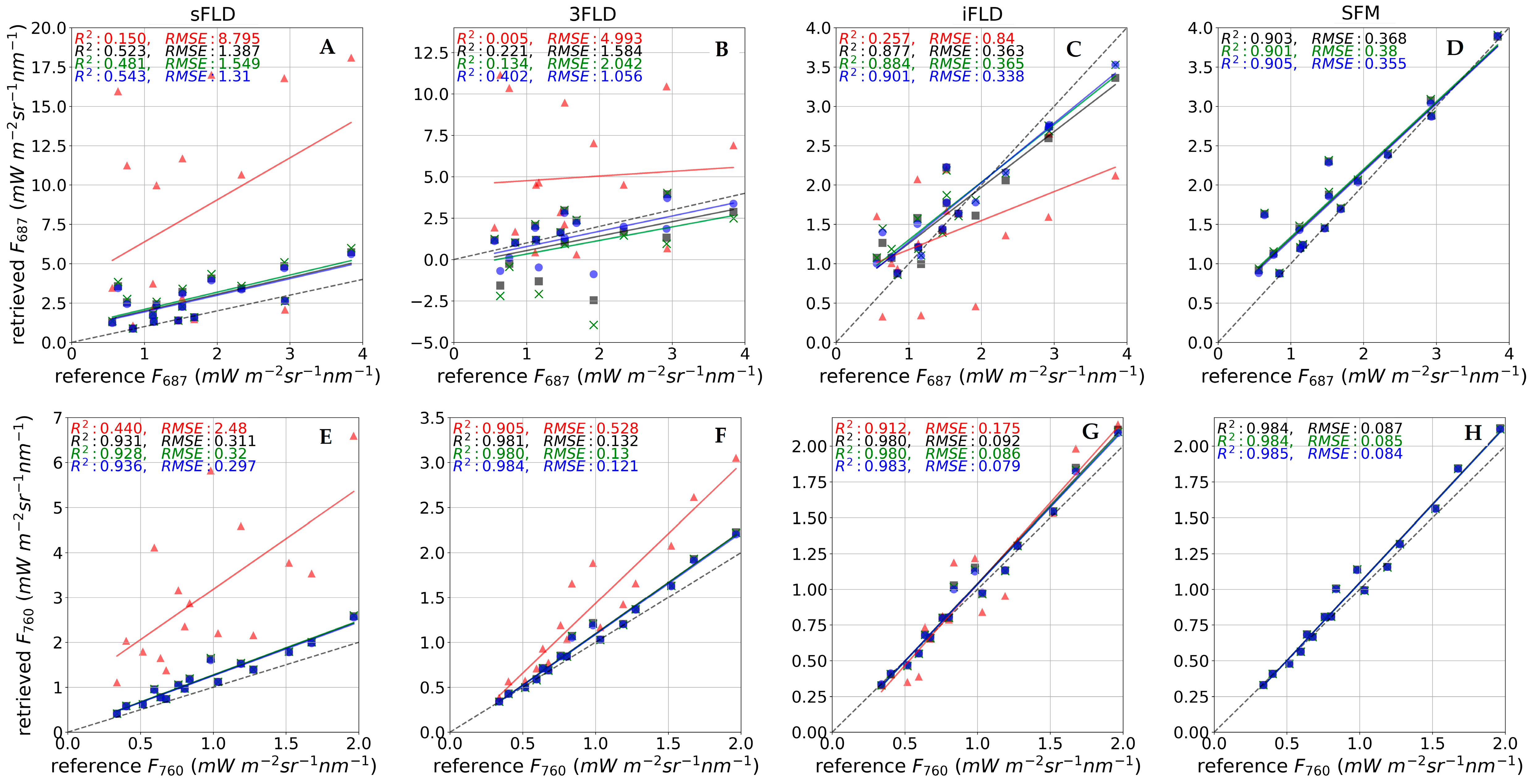
| ASD | 234.5 | 31.9 | 11.8 | --- | 370.1 | 101.9 | 41.2 | --- |
| QE Pro | 26.2 | 7.7 | 4.7 | 4.5 | 56.0 | 50.8 | 13.8 | 6.2 |
| MAYA | 33.4 | 14.4 | 7.0 | 4.9 | 62.9 | 50.8 | 10.4 | 7.2 |
| HR4000 | 40.9 | 25.4 | 9.6 | 4.8 | 66.5 | 34.5 | 9.7 | 5.9 |
| R2 | ||||||||
| ASD | 0.44 | 0.91 | 0.91 | --- | 0.15 | 0.00 | 0.26 | --- |
| QE Pro | 0.93 | 0.98 | 0.98 | 0.98 | 0.52 | 0.22 | 0.88 | 0.90 |
| MAYA | 0.93 | 0.98 | 0.98 | 0.98 | 0.48 | 0.13 | 0.88 | 0.90 |
| HR4000 | 0.94 | 0.98 | 0.98 | 0.99 | 0.54 | 0.40 | 0.90 | 0.91 |
| RMSE | ||||||||
| ASD | 2.48 | 0.53 | 0.18 | --- | 8.80 | 4.99 | 0.84 | --- |
| QE Pro | 0.31 | 0.13 | 0.09 | 0.09 | 1.39 | 1.58 | 0.36 | 0.37 |
| MAYA | 0.32 | 0.13 | 0.08 | 0.08 | 1.55 | 2.04 | 0.37 | 0.38 |
| HR4000 | 0.30 | 0.12 | 0.08 | 0.08 | 1.31 | 1.06 | 0.34 | 0.36 |
© 2019 by the authors. Licensee MDPI, Basel, Switzerland. This article is an open access article distributed under the terms and conditions of the Creative Commons Attribution (CC BY) license (http://creativecommons.org/licenses/by/4.0/).
Share and Cite
Cendrero-Mateo, M.P.; Wieneke, S.; Damm, A.; Alonso, L.; Pinto, F.; Moreno, J.; Guanter, L.; Celesti, M.; Rossini, M.; Sabater, N.; et al. Sun-Induced Chlorophyll Fluorescence III: Benchmarking Retrieval Methods and Sensor Characteristics for Proximal Sensing. Remote Sens. 2019, 11, 962. https://doi.org/10.3390/rs11080962
Cendrero-Mateo MP, Wieneke S, Damm A, Alonso L, Pinto F, Moreno J, Guanter L, Celesti M, Rossini M, Sabater N, et al. Sun-Induced Chlorophyll Fluorescence III: Benchmarking Retrieval Methods and Sensor Characteristics for Proximal Sensing. Remote Sensing. 2019; 11(8):962. https://doi.org/10.3390/rs11080962
Chicago/Turabian StyleCendrero-Mateo, M. Pilar, Sebastian Wieneke, Alexander Damm, Luis Alonso, Francisco Pinto, Jose Moreno, Luis Guanter, Marco Celesti, Micol Rossini, Neus Sabater, and et al. 2019. "Sun-Induced Chlorophyll Fluorescence III: Benchmarking Retrieval Methods and Sensor Characteristics for Proximal Sensing" Remote Sensing 11, no. 8: 962. https://doi.org/10.3390/rs11080962
APA StyleCendrero-Mateo, M. P., Wieneke, S., Damm, A., Alonso, L., Pinto, F., Moreno, J., Guanter, L., Celesti, M., Rossini, M., Sabater, N., Cogliati, S., Julitta, T., Rascher, U., Goulas, Y., Aasen, H., Pacheco-Labrador, J., & Mac Arthur, A. (2019). Sun-Induced Chlorophyll Fluorescence III: Benchmarking Retrieval Methods and Sensor Characteristics for Proximal Sensing. Remote Sensing, 11(8), 962. https://doi.org/10.3390/rs11080962