Gravity Recovery and Climate Experiment (GRACE) Storage Change Characteristics (2003–2016) over Major Surface Basins and Principal Aquifers in the Conterminous United States

Abstract

In this research, we characterized the changes in the Gravity Recovery and Climate Experiment (GRACE) monthly total water storage anomaly (TWSA) in 18 surface basins and 12 principal aquifers in the conterminous United States during 2003–2016. Regions with high variability in storage were identified. Ten basins and four aquifers showed significant changes in storage. Eight surface basins and eight aquifers were found to show decadal stability in storage. A pixel-based analysis of storage showed that the New England basin and North Atlantic Coastal Plain aquifer showed the largest area under positive storage change. By contrast, the Lower Colorado and California basins showed the largest area under negative change. This study found that historically wetter regions (with more storage) are becoming wetter, and drier regions (with less storage) are becoming drier. Fourier analysis of the GRACE data showed that while all basins exhibited prominent annual periodicities, significant sub-annual and multi-annual cycles also exist in some basins. The storage turnover period was estimated to range between 6 and 12 months. The primary explanatory variable (PEV) of TWSA was identified for each region. This study provides new insights on several aspects of basin or aquifer storage that are important for understanding basin and aquifer hydrology.

1. Introduction

Increased human activity has inevitably led to changes in the water cycle, especially water availability. Understanding changes in terrestrial water storage (sum of surface water storage, groundwater storage, soil moisture storage, canopy water storage, and snow water storage) is critical for the estimation of water availability in a region. The terrestrial water storage (TWS) is a fundamental component of a basin or continental water balance. However, there is still little understanding of this primary state variable [1], and its spatiotemporal variability is still emerging [2,3,4], primarily due to data scarcity of storage parameters—it is time consuming and challenging to conduct field campaigns over large areas [5]. Moreover, other problems, such as heterogeneous landscapes and basin complexities, introduce error while converting point-scale observations to the resolution of current large-scale hydrology and climate models [1]. Consequently, a continental-domain understanding of changes in basin storage remains elusive.

The first aspect of basin storage that requires investigation is understanding the spatiotemporal variability and the magnitude of storage change and its significance at different temporal scales. Most hydrologic studies assume storage change is insignificant at annual scales. However, several studies revealed that groundwater and other storage components of the hydrologic cycle often exhibit significant variability at seasonal and annual time scales [4,6,7,8]. Due to high variability and uneven distribution of hydrologic fluxes in space and time, basin storage could be significant even at annual time scales [1,4]. This is especially true in several regions where groundwater abstraction is a major component of the water budget. In such cases, assuming insignificant storage change could lead to inaccurate estimation of hydrologic fluxes. Hence, knowledge of spatiotemporal changes in storage and its importance with respect to basin precipitation is critical for understanding hydrologic behavior. Furthermore, in a changing world, both human impacts and climate variability could cause substantial changes in water availability [9]. Changes in water supply (precipitation and runoff distribution) and demand (human water consumption) lead to changes in inter- and intra-annual variability in basin storage and change the periodicity of storage and its turnover time in the basin. Hence, it is important to establish a baseline and monitor changes in storage over time. Another aspect to investigate is what drives the storage changes in a basin. TWS is generally driven or controlled by a combination of hydrologic fluxes. A study by Reager et al. [1] identified that there are differences among basins in terms of which flux drives TWS depending on precipitation, temperature, land cover, and soil moisture availability in the basin. However, we have an incomplete understanding on the interactions and dynamics of the various hydrologic drivers of TWS.

The Gravity Recovery and Climate Experiment (GRACE) mission is a joint National Aeronautics and Space Administration (NASA) and the German Deutsches Zentrum für Luft und Raumfahrt (DLR) project. GRACE provides direct global, monthly measurements of time-varying TWS changes and measures the temporal variations in the Earth’s gravity field. Wahr et al. [10] pointed out that GRACE gravity data can be used to recover water storage variations, but its coarser spatial resolution and accuracies inhibited the use of data over small basins and regions. Further research by Rodell and Famiglietti [6] showed that TWS accuracy could be improved by increasing the temporal interval and spatial resolution of the monitoring area (regions > 200,000 km²). The current Center for Space Research (CSR), University of Texas at Austin TWS dataset (CSR RL05 mascons) is an enhanced representation of the RL05 GRACE solutions and provides improved surface-based gridded information that can be used without further processing [11], providing an opportunity to use GRACE data for making regional water management decisions [12]. With availability of more than a decade of data (2003–2016) and improved data quality, GRACE TWS data have been used for addressing a wide range of questions. For example, GRACE storage data were used to identify extreme weather conditions, such as droughts [13,14] and floods [15,16], to analyze the impact of groundwater abstraction [17] and surface water storage [18], and more recently to understand the connections between large-scale weather patterns, such as the El Niño-Southern Oscillation (ENSO) and storage [19], and to understand hydro-climatic extremes [20,21].

Because of the importance of understanding this critical flux, several studies have analyzed basin TWS in the past using GRACE data. Apart from some continental and global studies [1,5,8,21,22], most studies have focused primarily on one or a few basins or regions [6,23,24,25,26,27,28]. Ramillien et al. [22] analyzed GRACE water mass variations over African basins and identified the potential of GRACE for management of water resources at the regional scale. Reager et al. [1] analyzed GRACE storage observations over several large basins globally. Their investigation included understanding variability in storage and analyzing hydrologic fluxes, such as precipitation, temperature, and land cover, as potential drivers of storage. Long et al. [5] performed global analysis of changes in the storage obtained from merged GRACE products. More recently, Scanlon et al. [8] compared GRACE TWS with global models in 186 river basins globally. Sun et al. [21] analyzed GRACE TWS over 35 basins globally to assess large-scale hydrologic extremes. However, these studies [1,5] covered only one or a few basins from the conterminous United States (CONUS), and storage changes over aquifers were not investigated. Furthermore, the relationship of storage with other hydrologic fluxes, such as basin runoff (Q), snow water equivalent (SWE), evapotranspiration (ET), and water balance (WB) in the CONUS region, is poorly characterized.

The goal of this study is to demonstrate myriad ways in which GRACE data can be used to improve our current knowledge on basin storage. Specific objectives of this study include analyzing GRACE storage for 18 surface basins and 12 aquifers to (a) characterize temporal variability and magnitude, (b) quantify periodicity or storage cycle, (c) identify primary hydrologic explanatory fluxes and controls of basin storage, and (d) estimate rate of change at both basin and pixel scales. The results from this study will advance current understanding of storage changes and enable resource managers to incorporate GRACE TWS in basin water-availability estimations and improve management of water resources.

2. Materials and Methods

2.1. Data Used

In this study we used 1° × 1° monthly GRACE RL05 mascon solutions obtained from the Center for Space Research, University of Texas (UT-CSR) (http://www2.csr.utexas.edu/grace) [11]. Mascon solutions provide a significant improvement in accuracy when compared to spherical harmonics data achieved through the reduction of leakage errors and reliable storage estimates in the tropics [11]. The UT-CSR mascon product was chosen because it shows gradual change along adjacent mascons as compared to sharp step changes between mascons in the unsmoothed Jet Propulsion Laboratory (JPL) mascon solutions [11]. Missing data were filled using the spline interpolation algorithm. The storage estimates obtained from the mascon product represent deviation of storage with respect to the mean period (2004–2009). The median obtained over 2003–2016 was subtracted from the monthly TWS mass deviations to obtain TWS anomaly (TWSA). This preserves the original magnitude and trend in storage. Therefore, the absolute value of storage denotes the deviation of storage from the decadal median storage estimate (2003–2016). We also derived month-to-month change in storage, ΔS, which is derived from TWSA, as described in a previous study [24] as:

$$\Delta S_t=TWS{A}_t-TWS{A}_{t-1}$$

(1)

where t and t − 1 are the current and previous months, respectively; ΔS_t is the monthly change in storage computed continuously for each month from January 2003–December 2016. Then, ΔS for a water year (ΔS_ANN) was estimated by adding monthly estimates from October to September for each year. Finally, a decadal mean annual estimate (ΔS_DM) for each basin was estimated using ΔS_ANN from all years.

The description of other datasets used in this study is presented here. Mean basin precipitation (P) over 2003–2016 was extracted from 4 km monthly parameter-elevation regressions on independent slopes model (PRISM) precipitation datasets [29,30] (http://prism.oregonstate.edu/historical/). Monthly basin runoff (Q) was extracted from gridded runoff data (2003–2016) obtained from the U.S. Geological Survey’s WaterWatch (https://waterwatch.usgs.gov/?id=romap3). Monthly regional evapotranspiration (ET) data were extracted from 1 km operational simplified surface energy balance algorithm (SSEBop) ET data (2003–2016) produced from model-assimilated weather datasets and Moderate Resolution Imaging Spectroradiometer (MODIS) thermal images [31] (https://earlywarning.usgs.gov/useta). Monthly snow water equivalent (SWE) was computed from Advanced Microwave Scanning Radiometer for Earth observing system (AMSR-E) L3 25 km ease grids (2003–2009) obtained from the National Snow and Ice Data Center [32] (http://nsidc.org/data/ae_mosno). Monthly soil moisture (SM) data (0–2 m) were obtained from National Land Data Assimilation System (NLDAS-2) monthly mosaic land surface model level 4 climatology data (0.125 × 0.125 degree) available from NASA (https://disc.gsfc.nasa.gov/datasets/NLDAS_MOS0125_MC_V002/summary) [33].

This study was carried out to understand the changes in storage over Hydrologic Unit Code 2 (HUC2) surface basins and principal groundwater aquifers in CONUS (Figure 1). The U.S. Geological Survey (USGS) has divided the United States into hydrologic units that are identified by unique numeric HUCs [34]. The entire United States is divided into 21 major surface regions (HUC2), composed of 222 sub-regions (HUC4) that are further divided into smaller basins (HUC6) and sub-basins (HUC8). The boundaries of these units are defined in terms of topographic river basin divides and sub-basins. The hydrologic unit code represents two digits each to indicate region, sub-region, basin, and sub-basin. In this study, we use 18 HUC2 surface basins covering CONUS. The approximate mean area of HUC2 is 500,000 km². Boundary information for all HUCs is obtained from the USGS (https://water.usgs.gov/GIS/huc.html). Twelve aquifers in the CONUS region were selected from the USGS Ground Water Atlas of the United States (https://water.usgs.gov/ogw/aquifer/atlas.html). The aquifer boundaries derived from this map indicate the areal extent of the uppermost principal aquifer system on a national scale. A principal aquifer system is a regionally extensive aquifer or aquifer system that has the potential to be used as a source of water abstraction for human or agricultural use.

2.2. Analysis of Temporal Variability and Magnitude in TWSA

Time series of TWSA are plotted to understand the temporal variability and magnitude of changes in the TWSA for HUC2 surface basins and principal aquifers. The goal of this exercise is to identify regions with high or low month-to-month, annual, and decadal variability in storage. Response of storage with respect to the climate variability (such as droughts and floods) is analyzed. We also validate the general assumption in hydrology—the significance of storage at annual and decadal scales. For each region, we identify the significance of storage by analyzing the mean ratio of annual ΔS_ANN and ΔS_DM with annual and decadal mean regional precipitation, respectively, during 2003–2016.

2.3. Analysis of Storage Cycle and Periodicity in Storage

First, we use an analytical approach to understand storage cycle using GRACE TWSA data. A simple algorithm was written that analyzes inflection points and turning points within the time series TWSA data to estimate average time (in months) of storage recharge and storage discharge and total time to complete one full cycle (recharge + discharge). A turning point is a point at which the TWSA derivative (slope) changes sign. The distance between two turning points can either be storage recharge period or storage discharge period, depending on the sign of the slope. A positive slope between the turning points indicates recharge period and a negative slope between two turning points indicates discharge period. This is an alternative approach to other robust algorithms [21,35] that delineate the storage cycle and periodicity in storage. However, any sudden anomalous change in TWSA slope (from positive to negative) with respect to the mean can result in a spurious or pseudo cycle, which would introduce noise or error in the estimation of the storage cycle. Hence, a 3-month moving average window was used to smooth out abrupt changes in the storage over certain months while preserving the annual and bi-annual cycles. The goal is to preserve the trend (annual and bi-annual trend) and reduce random noise in the monthly data. Analysis was performed using the mean estimate of TWSA for each of the HUC2 surface basins and aquifers. This approach is more analytical and does not provide statistical significance to the estimates of the storage cycle.

Second, we used a theoretical approach that provides statistical significance of the storage periodicity. The basin-averaged TWSA was transformed into frequency domain to investigate the dominant frequencies in the GRACE storage signal [1]. Fourier analysis of the storage time series data was undertaken to identify the dominant periodic cycles. Plots of periodograms, which are plots of the relative power spectra of individual periodic components, are used for visual interpretation. Usually, hydrological time series data are a combination of signals with multi-year, annual, and sub-annual cycles. As the relative power of the annual and multi-annual components are higher in a given TWSA time series, sub-annual components are relatively subdued. To enhance the sub-annual components and improve visibility and clarity, we used the month-to-month change in storage (ΔS) parameter, which effectively filters out the relative strong multi-annual power component from the data. The 95% confidence intervals were generated, using white noise spectra with mean of the distribution and two standard deviations of the spectra (for both TWSA and ΔS), and plotted along with the periodograms. If the power of the signal lies above the 95th percentile confidence interval of the white noise spectra, then it is considered statistically significant and different from white noise.

2.4. Analysis of Primary Explanatory Variable of Storage

To understand the hydrologic fluxes that can explain the GRACE storage signal, we investigated five independent fluxes and storage terms (P, ET, Q, SWE, SM, and WB = P-ET-Q) against the GRACE storage signal (dependent variable). Direct comparison of hydrologic fluxes with GRACE TWSA is not possible because hydrologic fluxes are direct measures, whereas the latter is an anomaly. Hence, we computed an anomaly for each hydrologic flux and storage term as a deviation from the decadal median and compared it with GRACE TWSA in the following ways: (i) the behavior of TWSA against the hydrologic variables was analyzed for each basin; (ii) using decadal mean monthly TWSA estimates produced from the 2003–2016 data, a stepwise regression was performed to identify the best model (with lowest Akaike information criterion, AIC), and a set of parameters in the best model for each basin was identified; and (iii) hydrologic variables with highest correlation with TWSA were identified. Generally, presence of multicollinearity results in extremely unstable regression coefficients which could cause serious problems when making inferences and predictions based on the regression model [36]. Hence, we used a multicollinearity diagnostic test for each regressor (explanatory variables) using “MCTEST” package in R and estimated multicollinearity in the model using the variance inflation factor (VIF). Usually, a VIF > 10 is a common threshold for detecting severe multicollinearity [37], and thus any variable with VIF > 10 will be ignored. For efficient management of basin water storage, it is important to identify the primary explanatory variables of storage. Hence, we computed the contribution of each variable in the best fit model using standardized partial regression coefficients, and the variable with the highest contribution was identified.

2.5. Analysis of Change in Storage

Several regional studies in the past have used GRACE TWS to understand change in storage over time [5] and decadal trends in TWS, for example, groundwater depletion in India [38,39] and TWS changes in the U.S. in California’s Central Valley [40,41] and in the High Plains aquifer region [41,42]. More recently, GRACE-derived TWS was used to estimate emerging trends in global freshwater availability [4]. Most of these studies have provided estimates of rate of change (mm/year) in storage obtained from GRACE. In this study, we perform the seasonal Mann-Kendall (SMK) test [43], using “rkt” package in R statistical software, using monthly GRACE TWSA over 2003–2016. For each basin, the Theil-Sen’s slope and 5% significance level (p-val ≤ 0.05) were estimated. For easy interpretation, we converted significance levels to directional p-val (containing both positive and negative p-val) based on the direction of the slope. This analysis of change in storage was performed both at the basin scale and at the pixel level to identify regions showing significant changes in storage.

3. Results

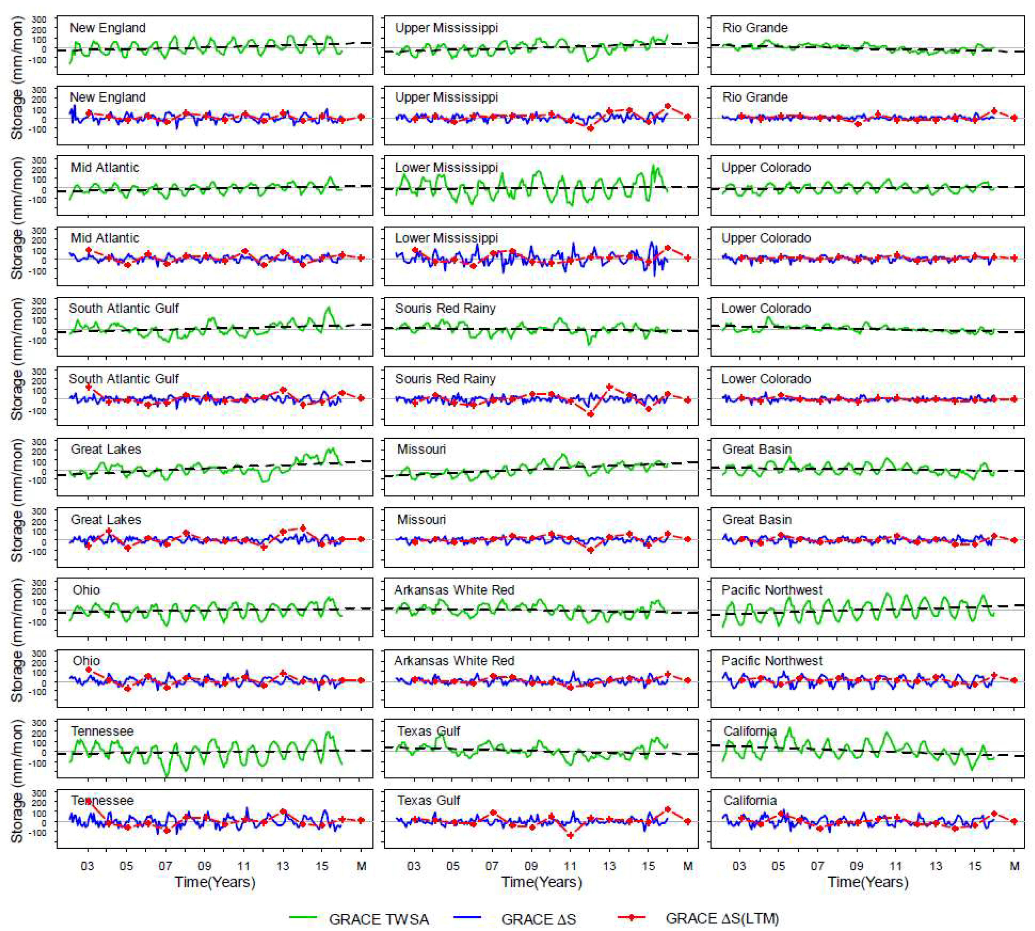
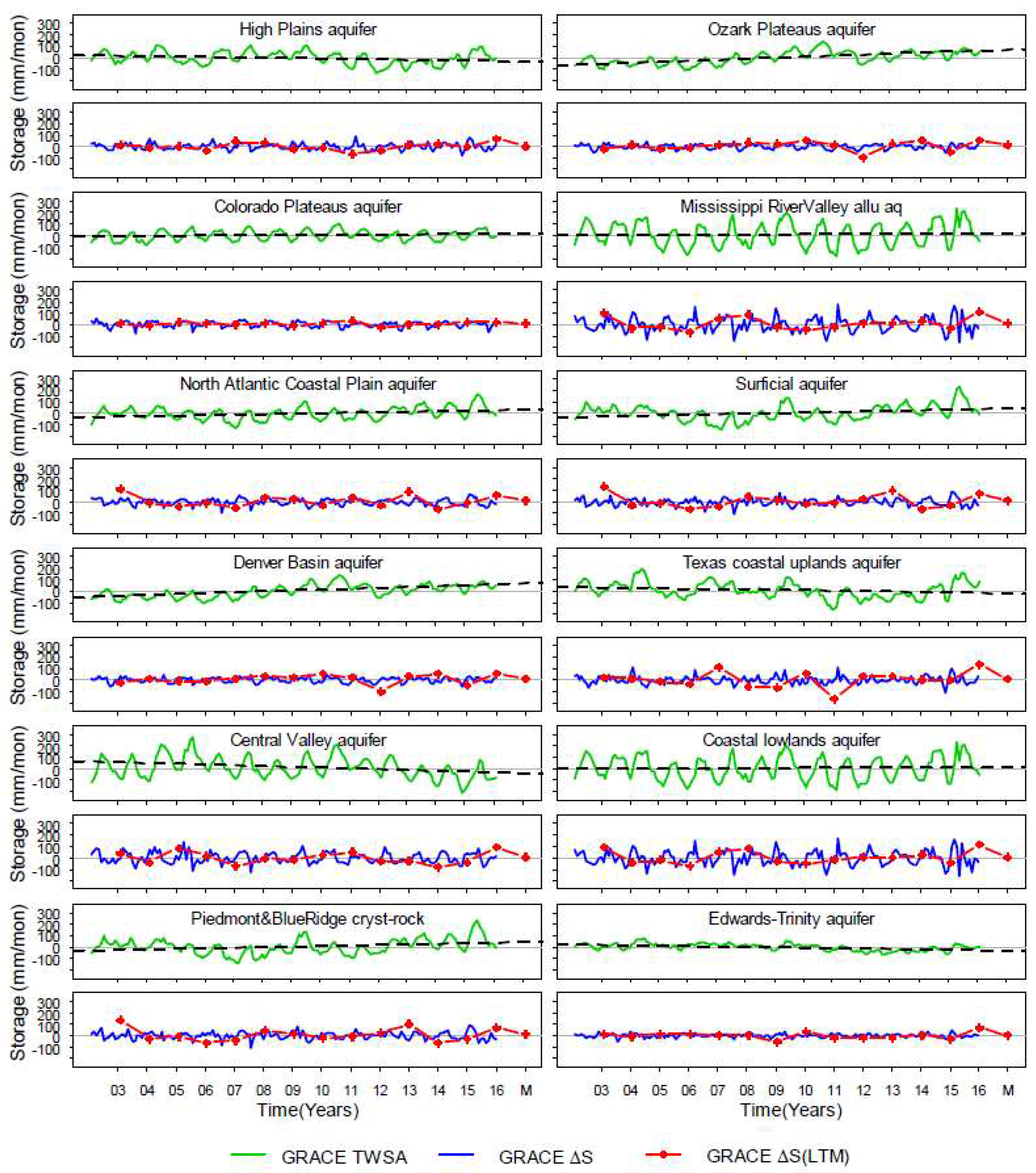
3.1. Analysis of Temporal Variability and Magnitude in Storage (2003–2016)

The temporal variability in monthly TWSA (green line), ΔS (blue line), and ΔS_{Ann, DM} (red line) for HUC2 surface basins and principal aquifers over 2003–2016 are presented in Figure 2 and Figure 3. Monthly TWSA demonstrates seasonal variability, and the slope (dashed line) is a good indicator of long-term trend. Coefficient of variability, CV ((Standard Deviation * 100) / Mean of the observation), was computed on TWSA to understand the combined monthly and decadal variability (with respect to the mean storage) in each basin or aquifer. TWSA variability for 4 out of 12 surface basins (Great Lakes, Tennessee, Texas-Gulf, and California) showed low variability (CV < 10%). Similarly, TWSA variability for 6 out of 12 aquifers (High Plains aquifer, Mississippi River alluvial aquifer, Surficial aquifer, Texas Coastal Uplands aquifer, North Atlantic Coastal Plain aquifer, and Denver Basin aquifer) showed high variability (CV > 20%). On the other hand, the Coastal lowlands aquifer and Ozark Plateaus aquifer showed low variability (CV < 10%). These results were different when ΔS was used to compute CV with a focus on quantifying month-to-month variability (not shown here). GRACE TWSA data were also found to capture variability due to climate extremes. A wet year results in an increase in storage due to high precipitation and increased water availability. For example, the Missouri River basin experienced catastrophic floods during 2011, and the GRACE TWSA signal for 2011 showed an all-time high in storage over 2003–2016. Similar peaks in storage during wet periods can also be seen in other basins, such as prolonged floods in the South Atlantic Gulf basin in 2015 and floods in Texas in 2004. A general increase in Great Lakes water levels, as indicated by the altimetry data (https://ipad.fas.usda.gov/cropexplorer/global_reservoir/), corroborates an increase in storage in the Great Lakes region. Similarly, a dry season results in loss of storage due to low precipitation, high evapotranspiration, and reduced groundwater levels. For example, the GRACE TWSA signal for Tennessee showed an all-time low storage due to the extreme drought in 2007. Similar declines in storage during dry periods can also be seen in other basins experiencing drought, such as California (2011–2015) and Texas (2011). Figure 2 and Figure 3 also demonstrate that there is high variability in inter- and intra-annual storage among HUC2 surface basins and aquifers.

The ΔS was found to demonstrate only the monthly variability. For most basins and aquifers, ΔS was found to oscillate around zero with low CV and was devoid of any decadal trend. The Great Lakes basin and California basin showed the lowest CV in ΔS. The low CV could be because the Great Lakes basin is the least disturbed basin, and hence has low variability, whereas the California basin is highly managed and variability is under control due to water management practices. However, 5 out of 18 surface basins (South Atlantic Gulf, Missouri, Arkansas-White-Red, Upper Colorado, and Pacific Northwest) show high variability (CV > 20%), indicating very large fluctuations in storage on a monthly basis. Although the annual change in storage (ΔS_ANN) was usually close to zero for most years, it was found to be considerably different from zero for some years. This means that the change in storage was not equal to zero on an annual basis. On a decadal scale, ΔS_DM (value for “M” on axis) was found to be close to zero, indicating that although ΔS_ANN may not be zero at an annual time scale, it is close to zero (insignificant) at longer time scales.

As storage changes depend on precipitation in a given region, we computed the ratio of annual ΔS/P for each region to understand the significance of change in storage within the water budget. The annual ΔS/P percent (in

Table 1. Analysis of the ratio of month-to-month change in storage and P (ΔS/P) annual max, min, and decadal mean (DM) for each region to understand the significance of change in storage in the water budget.

HUC 2 Surface Basins	Annual ΔS/P (%)			Aquifer	Annual ΔS/P (%)
	Max	Min	DM		Max	Min	DM
New England	0.7	−0.7	0.05	High Plains	0.8	−2.4	−0.10
Mid−Atlantic	0.7	−0.9	−0.01	Colorado Plateaus	1.1	−0.9	0.02
South Atlantic Gulf	0.9	−0.9	0.01	N Atlantic Coastal Plain	0.7	−1.0	0.00
Great Lakes	1.1	−1.1	0.05	Denver Basin	0.6	−0.6	−0.02
Ohio	1.2	−1.2	0.06	Central Valley	5.4	−9.9	−1.28
Tennessee	1.7	−1.8	0.03	Piedmont and Blue Ridge Cryst. Rock	0.9	−1.4	0.01
Upper Mississippi	1.1	−1.7	0.04	Ozark Plateaus	1.4	−0.8	0.09
Lower Mississippi	1.1	−1.0	0.03	Mississippi River Valley	1.6	−1.2	0.06
Souris−Red−Rainy	1.5	−3.9	−0.28	Surficial	0.8	−1.0	0.00
Missouri	0.9	−2.5	0.02	Texas Coastal Uplands	1.7	−4.4	−0.20
Arkansas−White−Red	0.7	−1.5	−0.06	Coastal Lowlands	0.7	−1.2	−0.01
Texas Gulf	1.3	−5.3	−0.32	Edwards Trinity	1.2	−8.7	−0.57
Rio Grande	0.8	−3.7	−0.26
Upper Colorado	1.3	−1.1	0.04
Lower Colorado	1.2	−1.6	−0.20
Great Basin	1.9	−1.8	−0.17
Pacific Northwest	1.1	−0.9	0.07
California	2.2	−3.2	−0.35

Note: DM is the decadal mean estimate of annual ΔS/P and Max and Min indicate maximum and minimum year-to-year changes in the ΔS/P.

) indicates that change in annual ΔS varies between ±10% of the annual P, as indicated by the minimum and maximum annual ΔS/P during 2003–2016. At an annual time scale, 5 out of 18 HUC2 surface basins (Souris-Red-Rainy, Missouri, Texas Gulf, Rio Grande, and California) and 4 out of 12 principal aquifers (Central Valley, High Plains, Texas Coastal Uplands, and Edwards Trinity) showed substantial storage (max > 2%; min < 2%). However, on a decadal time scale, the ΔS/P (DM) was found to be small (less than ±2% of basin P). This result confirms the validity of the general assumption in hydrology that storage is insignificant at longer time scales (decadal or more).

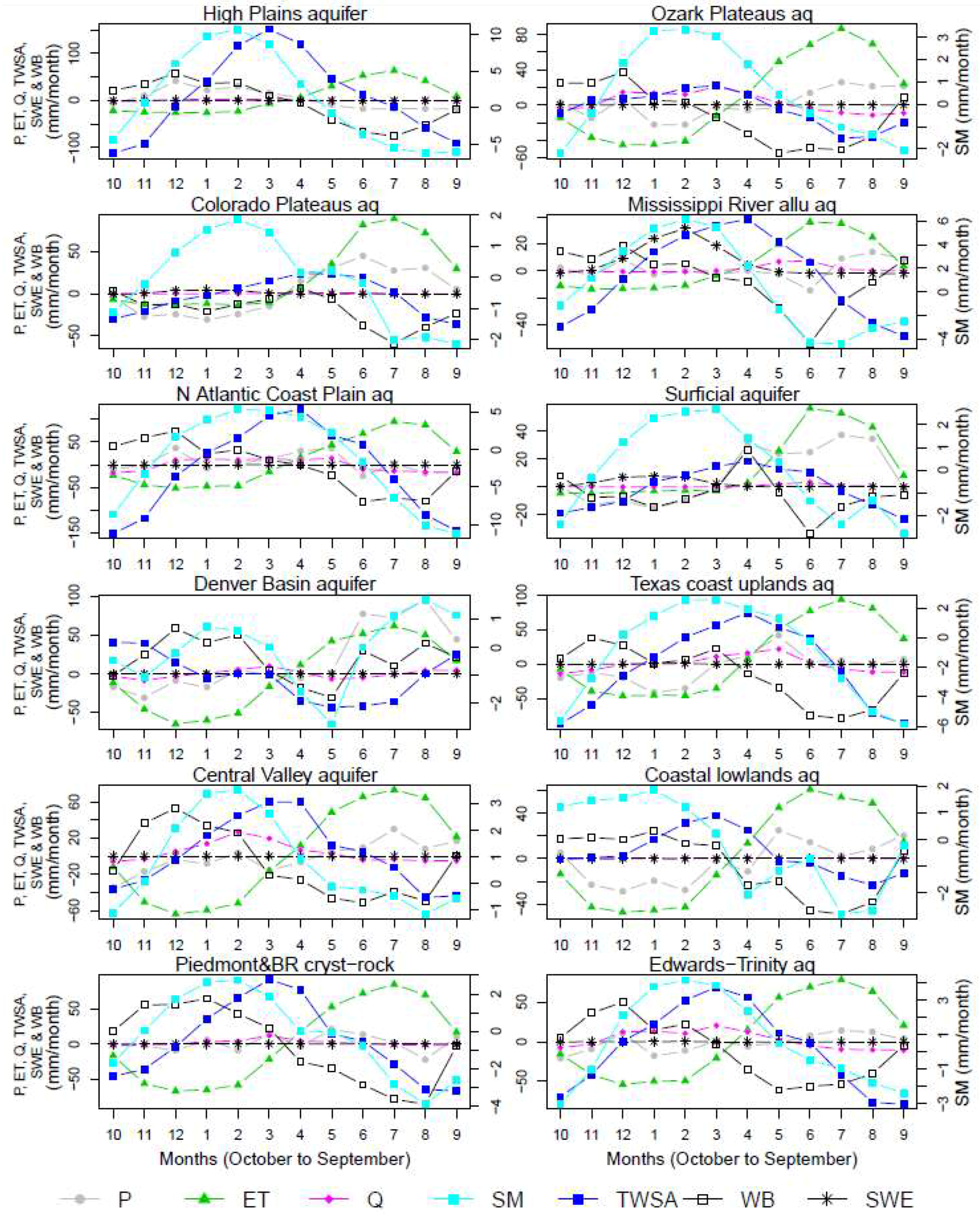
3.2. Analysis of Storage Cycle and Periodicity in Storage

Results of analysis of storage cycle are presented in

Table 2. Estimates of average storage cycle (STP) and ± standard deviation (SD) in months derived for surface basins and aquifers using GRACE TWSA.

HUC2 Surface Basins	Average STP ± SD (Months)	Aquifers	Average STP ± SD (Months)
New England	12 ± 1	High Plains	10 ± 3
Mid-Atlantic	12 ± 1	Colorado Plateaus	12 ± 1
South Atlantic Gulf	9 ± 4	N Atlantic Coastal Plain	12 ± 2
Great Lakes	10 ± 3	Denver Basin	10 ± 3
Ohio	12 ± 1	Central Valley	12 ± 1
Tennessee	11 ± 2	Peidmont and BR cryst-rock	9 ± 4
Upper Mississippi	10 ± 3	Ozark Plateaus	10 ± 3
Lower Mississippi	11 ± 2	Mississippi River Valley	12 ± 3
Souris-Red-Rainy	10 ± 3	Surficial aquifer	9 ± 3
Missouri	10 ± 3	Texas Coastal Uplands	7 ± 4
Arkansas-White-Red	10 ± 3	Coastal lowlands	12 ± 3
Texas Gulf	7 ± 4	Edwards-Trinity	6 ± 3
Rio Grande	6 ± 3
Upper Colorado	12 ± 1
Lower Colorado	9 ± 3
Great Basin	12 ± 1
Pacific Northwest	12 ± 1
California	12 ± 1

Note: Average STP is equally divided into storage recharge period (SRP) and storage discharge period (SDP).

. Storage cycle analysis indicated that HUC2 surface basins in CONUS took 6 to 12 months to complete a storage cycle, but with high year to year variability (standard deviation up to 4 months). Nine out of 18 basins showed average storage cycles of 12(±1) months. However, 9 basins showed average storage cycles of <12 months. The Rio Grande (6 months) and Texas Gulf (7 months) both showed bimodality of storage. The storage cycle analysis of aquifer systems revealed that it took 6 to 12 months to complete a storage cycle. However, only 5 out of 12 aquifer systems showed annual storage cycles (12 ± 1 months) and the rest (7 out 12) of the aquifer systems took <12 months to complete a storage cycle. The Edwards-Trinity and Texas Coastal Uplands aquifer systems showed bimodal storage cycles within a period of 12 months.

Results from the Fourier analysis of the basin-averaged GRACE signal (periodograms) are presented in Figure 4 and Figure 5. To establish statistical significance of these peaks, we generated white noise using the mean and standard deviation of the observation, and we plotted a 95th percentile confidence interval of the white noise spectra (red and dashed lines in Figure 4 and Figure 5). Any peak lying above the 95th percentile confidence interval is considered significantly different from the white noise. Fourier transformation of GRACE TWSA and ΔS signals showed prominent annual and multi-annual peaks and subdued sub-annual peaks. Fourier analysis of both TWSA and ΔS signals reveals that all basins and aquifers show a prominent annual cycle with a statistically significant peak at a frequency of 1 cycle/year. However, the signal from TWSA indicated prominent multi-annual cycle peaks for 7 out of 12 HUC2 surface basins (South Atlantic Gulf, Great Lakes, Souris-Red-Rainy, Missouri, Arkansas-White-Red, and Texas Gulf). Fourier analysis of ΔS showed amplified signals at sub-annual scales and high frequencies. Additional peaks in ΔS at higher frequencies were also seen for 7 out of 18 basins (Great Lakes, Ohio, Upper Mississippi, Souris-Red-Rainy, Missouri, Rio Grande, and Lower Colorado) and showed prominent higher order frequencies (sub-annual cycles). The presence of significant higher order frequencies could mean that in addition to prominent annual periodicity, portions or regions within the basins exhibit sub-annual storage periodicities. Identifying and understanding the presence of high spatial variability in storage periodicity within a basin is important for basin water management. Since this analysis uses monthly data, we ignore frequencies > 6 cycles/year and frequencies < 1/14 cycles/year. Fourier analysis revealed similar results for aquifer systems with prominent annual cycles (frequency of 1 cycle/year). However, 4 out of 12 aquifers (Peidmont and Blue Ridge crystalline rock aquifer, Ozark Plateaus aquifer, Surficial aquifer, and Texas Coastal Uplands aquifer) showed statistically significant peaks at cycles >1/year. Fourier analysis of ΔS showed that 3 out of 12 aquifers (High Plains aquifer, Surficial aquifer, and Edwards-Trinity aquifer systems) showed sub-annual periodicities (cycles) of storage.

3.3. Analysis of Primary Explanatory Variable of Storage

The decadal monthly GRACE TWSA derived from the water year (October–September) data during 2003–2016 is plotted against other hydrologic fluxes (computed as deviation from decadal median) in Figure 6 and Figure 7. Visual comparison of TWSA in most of the basins indicates a general trend of minimal storage in October and increasing storage in winter (November–April), and then decreasing storage in summer (April–September). This general trend in TWSA did not respond to P in most basins, as higher P in summer did not translate into higher basin storage. This could be because basin ET was found to be more than P during summer. Higher ET often results in loss of surface water, resulting in a decrease in net storage; therefore, storage showed a negative relationship with ET. For most regions, storage tends to increase until WB is positive (above its decadal median), and as ET tends to increase in summer, storage tends to decline. Runoff and SWE showed a weak relationship with storage in most of the basins. However, SWE from winter months showed a positive relationship with ΔS in some basins. Although magnitude of monthly change in soil moisture was low for most basins, it followed the general trend of storage, and hence showed a positive relationship with basin storage (Figure 6 and Figure 7). To understand the interaction between hydrologic fluxes and TWSA, we computed TWSA response lag on each variable (see

Table A1. Analysis of TWSA lag against other hydrologic variables.

No	Basin Name	P-TWSA	SM-TWSA	Q-TWSA	ET-TWSA	SWE-TWSA
HUC2 Surface Basins
1	New England	5	1	−1	−4	2
2	Mid−Atlantic	−6	1	0	−4	1
3	South Atlantic Gulf	−5	1	0	−4	2
4	Great Lakes	1	4	2	−1	4
5	Ohio	−2	1	0	−4	1
6	Tennessee	−1	2	3	−3	4
7	Upper Mississippi	−2	1	0	−3	3
8	Lower Mississippi	−1	2	2	−3	−1
9	Souris−Red−Rainy	−3	0	−1	−4	1
10	Missouri	−1	2	−1	−2	4
11	Arkansas−White−Red	−2	2	−1	−3	4
12	Texas−Gulf	−3	2	1	−4	2
13	Rio Grande	−4	2	−2	−4	2
14	Upper Colorado	6	1	−2	−3	3
15	Lower Colorado	−5	1	1	−4	2
16	Great Basin	4	2	−1	−3	3
17	Pacific Northwest	4	2	−1	−3	4
18	California	3	1	0	−4	2
Aquifers
1	High Plains	3	1	0	−4	3
2	Colorado Plateaus	−2	2	−2	−3	3
3	N Atlantic Coastal Plain	−1	2	−1	−3	2
4	Denver Basin	−10	−10	−5	−9	−1
5	Central Valley	−4	1	1	−4	5
6	Piedmont and Blue Ridge	−2	1	0	−4	3
7	Ozark Plateaus	−4	1	0	−4	1
8	Mississippi River Valley	−4	2	−2	−2	2
9	Surficial	−3	1	−2	−2	3
10	Texas Coastal Uplands	−1	1	−1	−3	2
11	Coastal Lowlands	−2	2	−2	−3	2
12	Edwards−Trinity	−4	1	0	−4	1

Note: Lag—storage lag in months. A negative lag of “n” months indicates that TWSA is reaching its peak “n” months prior to the variable or (12-n) months after the variable reaches its peak. A positive lag of “n” indicates that TWSA is reaching its peak “n” months after the variable reaches the peak; r indicates the correlation of TWSA and variable at lag “n”. NA denotes that SWE volumes were low, and hence excluded from the computation of lags.

). Our results indicate that despite P being the main driver of hydrologic processes, TWSA responds with P with a greater lag than other variables, mainly because it depends on the way P is partitioned into hydrologic fluxes (such as SM, ET, Q, and SWE). However, for most basins, soil moisture and runoff had quicker response times on TWSA. For example, in the South Atlantic Gulf basin (Figure 6), precipitation occurs for almost all months, with most of the precipitation falling in the summer months (peaking in August). During summer, theoretically, other fluxes and storage, such as soil moisture, runoff, and TWSA, should increase, but in fact, these fluxes decrease in summer. This decrease occurs because most of the P is meeting the ET demand from vegetation. During winter and spring (October–April), ET is low, and hence soil moisture is increasing, as is TWSA. While SM attains a peak in February, TWSA continues to peak until March. Runoff shows greater response to TWSA with a lag of 0. Hence, for the South Atlantic Gulf, runoff is a key explanatory variable of TWSA. Most of the other basins also have similar responses with runoff and soil moisture showing greater response (smaller lag) to TWSA. Other than soil moisture and runoff, the key driver of TWSA is ET. For most basins, the zero crossing of ET (when the monthly ET starts to increase beyond the long-term mean) corresponds to the peak of TWSA, which means any increase in ET mostly leads to a decline in TWSA.

Stepwise regression analysis results, partial regression coefficients, and the primary explanatory variable for each region (HUC2 surface basins and aquifer systems) are presented in

Table 3. Stepwise regression approach to identify a set of explanatory variables (Precipitation, P; Runoff, Q; Snow Water Equivalent, SWE; Evapotranspiration, ET; and soil moisture, SM) and a primary explanatory variable (PEV) of GRACE TWSA in the CONUS.

ID	Basin	Partial Regression Coefficients (%) for the Variables in the Best Fit Model					Model adj. R2	PEV	Individual r (TWSA vs. PEV)
		P	Q	ET	SWE	SM
HUC 2 Basins
1	New England	2	2	NA	2	93	0.98 *	SM	0.96
2	Mid-Atlantic	NA	NA	1	2	97	0.97 *	SM	0.97
3	South Atlantic Gulf	31	34	1	0.5	20	0.95 *	Q	0.93
4	Great Lakes	15	NA	17	NA	68	0.96 *	SM	0.42
5	Ohio	1	NA	NA	NA	99	0.97 *	SM	0.98
6	Tennessee	NA	NA	5	NA	95	0.92 *	SM	0.94
7	Upper Mississippi	NA	48	7	4	41	0.98 *	Q	0.88
8	Lower Mississippi	NA	NA	12	NA	88	0.93 *	SM	0.74
9	Souris-Red-Rainy	NA	30	12	21	37	0.96 *	SM	0.63
10	Missouri	1	NA	22	1	69	0.96 *	SM	0.61
11	Arkansas-White-Red	10	30	19	3	38	0.95 *	SM	0.84
12	Texas-Gulf	13	75	NA	12	NA	0.76 *	Q	0.73
13	Rio Grande	26	NA	NA	22	52	0.67 *	SM	0.57
14	Upper Colorado	NA	6	19	NA	75	0.96	SM	0.67
15	Lower Colorado	12	88	NA	NA	NA	0.82 *	Q	0.85
16	Great Basin	NA	5	16	4	75	0.94 *	SM	0.64
17	Pacific Northwest	NA	NA	16	6	78	0.56 *	SM	0.77
18	California	NA	89	NA	11	NA	0.87 *	Q	0.89
Principal aquifers
1	Central Valley	NA	82	NA	NA	18	0.84 *	Q	0.82
2	High Plains	NA	88	NA	12	NA	0.77 *	Q	0.84
3	Missi. River Valley	NA	NA	17	NA	83	0.88 *	SM	0.88
4	Surficial	NA	NA	100	NA	NA	0.37 *	ET	−0.59
5	Coastal Lowlands	NA	92	8	NA	NA	0.66 *	Q	0.82
6	Texas Coastal Uplands	NA	32	14	NA	54	0.88 *	SM	0.77
7	N Atlantic Coast. Plain	22	69	9	NA	NA	0.90 *	Q	0.9
8	Colorado Plateaus	NA	36	NA	64	NA	0.66 *	SWE	0.6
9	Denver Basin	4	12	NA	6	78	0.88 *	SM	0.66
10	Ozark Plateaus	NA	NA	6	2	92	0.96 *	SM	0.93
11	Edwards-Trinity	60	40	NA	NA	NA	0.54 *	P	−0.53
12	Piedmont and BR	1	73	22	4	NA	0.90 *	Q	0.9

Note: NA denotes variable not used in the regression model (omitted due to multicollinearity); * model significant at 0.05 level.

. Variables discarded due to multicollinearity and those that are not identified in the best fit model are represented as “NA”. For all the basins, the existence of the WB term resulted in high multicollinearity, because WB is a derivative of other hydrologic fluxes (P, Q, and ET), hence WB was removed from the analysis.

Results indicated that SM was found to be the primary explanatory variable of storage in 13 of the 18 HUC2 surface basins. Runoff (Q) was found to explain storage patterns in 5 basins (South Atlantic Gulf, Upper Mississippi, Texas Gulf, Lower Colorado, and California). With respect to storage changes in the aquifer systems, we have mixed results. Runoff was found to explain storage changes in 5 out of 12 aquifers (Central Valley, High Plains, Coastal lowlands, North Atlantic Coastal Plain, and Piedmont and Blue Ridge crystalline-rock aquifers). Soil moisture (SM) was found to explain storage changes in four aquifers (Mississippi River valley aquifer, Texas Coastal Uplands, Denver Basin, and Ozark Plateaus aquifers). The fluxes ET and SWE were found to be primary explanatory variables in the Surficial aquifer and Colorado Plateaus aquifers, respectively. Precipitation (P) was found to be the primary explanatory variable for the Edwards-Trinity aquifer. Fluxes Q, SWE, and SM exhibited positive individual correlation with storage. However, P showed a negative relationship due to the lagged response of TWSA. Evapotranspiration showed an expected negative correlation, indicating that high ET corresponds to decline in storage, and vice versa.

3.4. Analysis of Change in Storage

Theil-Sen’s slope estimate obtained from the Mann-Kendall analysis of TWSA data (2003–2016) yielded rate of change estimates for each region (

Table 4. Rate of change (cm/year) in storage and surface area under change derived using GRACE TWSA data (2003-2016) for HUC2 surface basins and principal aquifers in the CONUS.

No	Name	GRACE TWSA		Basin/Aquifer Area (%) under
		Rate of Change (cm/yr)	P value	Negative Change	Positive Change	No Change
HUC2 Surface Basins
1	New England	4.3	0.0009	2	98	0
2	Mid-Atlantic	3.8	0.0188	0	77	23
3	South Atlantic Gulf	5.9	0.2232	0	25	75
4	Great Lakes	8.8	0.0348	5	63	32
5	Ohio	4.2	0.0431	0	56	44
6	Tennessee	3.1	0.4078	0	3	97
7	Upper Mississippi	7	0.0298	3	74	23
8	Lower Mississippi	1.7	0.6456	1	5	94
9	Souris-Red-Rainy	−2.1	0.3875	31	6	63
10	Missouri	9.9	0.003	0	82	18
11	Arkansas-White-Red	−4.6	0.2361	32	1	67
12	Texas-Gulf	−6	0.2196	14	0	86
13	Rio Grande	−5.1	0.0104	67	0	33
14	Upper Colorado	1.8	0.2267	3	31	66
15	Lower Colorado	−4.9	0.003	79	0	21
16	Great Basin	−2.8	0.1774	18	3	79
17	Pacific Northwest	7.9	0.0006	1	86	12
18	California	−9.1	0.0279	60	7	33
Principal Aquifers
1	High Plains	−4.1	0.2304	33	40	26
2	Colorado Plateaus	1.5	0.2475	20	19	61
3	N Atlantic Coastal Plain	3.9	0.1332	0	63	38
4	Denver Basin	10	0.0023	17	17	67
5	Central Valley	−8.8	0.0332	80	0	20
6	Piedmont and Blue Ridge crystalline-rock	5.3	0.2451	0	5	95
7	Ozark Plateaus	10	0.0023	0	33	68
8	Mississippi River Valley alluvial	1.4	0.6005	0	11	89
9	Surficial	5.3	0.2451	0	52	48
10	Texas Coastal Uplands	−5.6	0.2406	0	0	100
11	Coastal lowlands	1.4	0.6005	0	0	100
12	Edwards-Trinity	−4.9	0.0118	7	0	93

Note: directional p-val shown in italics are significant at 95% confidence level.

). Seven out of 18 basins showed large increases in storage and 3 basins (in the western United States) showed large decreases in storage. The highest significant rate of change in storage was found in the Missouri (9.9 cm/year), followed by the Great Lakes (8.8 cm/year) and Pacific Northwest (7.9 cm/year) basins. The largest decline in storage occurred in the California basin (−9.9 cm/year). For the aquifer systems, only two aquifers (Denver Basin and Ozark Plateaus) showed large increases in storage (10 cm/year each); the Central Valley and Edwards-Trinity aquifers showed large declines in storage (−8.8 and −4.9 cm/year, respectively).

Analysis of change in storage at basin or aquifer scale provides information on overall change occurring in the region. However, it does not provide information on spatial variability in storage change within a region. Hence, pixel-scale analysis of rate of change in storage is presented in Figure 8 (top graphics). Although some basins showed overall significant ± changes in GRACE storage, not all areas within these basins or aquifers showed significant ± change in storage. Regions shaded in blue indicate positive rates of change and regions shaded in yellow to brown indicate negative rates of change. Figure 8 (bottom graphics) shows areas that are statistically significant at the 95% (0.05) level. Parts of the Missouri, Pacific Northwest, Upper Mississippi, Great Lakes, and South Atlantic Gulf regions show significant positive changes in storage. Similarly, northern parts of the High Plains aquifer and Surficial aquifer show significant positive changes in storage (Figure 8). Regions in southwestern CONUS covering parts of the California, Lower Colorado, Rio Grande, and Arkansas-Red-Rainy basins and the northwestern tip of the Texas Gulf basin show significant negative changes in storage (Figure 8). These regions are characterized by arid to semi-arid conditions, where precipitation is scarce and groundwater irrigation is common. The negative change in storage is more prominent along the Central Valley and southern High Plains aquifer regions (Figure 8), where irrigation is predominant. This regionalized information on changes in GRACE storage can be helpful for water resource managers. Based on the statistical probability estimates, we computed the area under change (positive, negative, or no change) for each region. Results presented in Table 4 indicate that for the New England basin, 98% of the basin experiences an increase (positive change) in storage. Conversely, 79% of the Lower Colorado basin experiences a negative change (decrease in storage). On the other hand, the Tennessee and Lower Mississippi basins are stable with no significant changes occurring during 2003–2016 in >90% of the basin areas, while small areas of the basins experience a negative change. Similarly, the North Atlantic Coastal Plain and Surficial aquifers show >50% of their areas under increasing change in storage; nearly 80% of the Central Valley aquifer experiences negative change in storage. The Texas Coastal Uplands and Coastal lowlands aquifers demonstrate stability in storage, with 100% of these aquifer systems having no change in storage during 2003–2016.

4. Discussion

In this study, we used monthly GRACE CSR RL05 mascons and derived TWSA, ΔS_ANN, and ΔS_DM, as described in Section 2.1. This study demonstrates that each of these derivatives of storage parameters provide useful and sometimes supplemental information on storage characteristics. However, care should be exercised in the use of these parameters. For example, TWSA is important in understanding annual and decadal variability with respect to the mean period (2003–2016); however, TWSA would be of little use in understanding information on the actual magnitude of month-to-month change in storage, which is provided by ΔS. For this reason, TWSA should not be used in analyses or studies that require absolute estimates of storage or storage change. For example, to understand the significance of monthly change in storage with respect to the basin P (or other hydrologic fluxes), ΔS should be used instead of TWSA. Similarly, since TWSA is an anomaly term, it should not be directly compared with hydrologic fluxes. However, since ΔS provides absolute estimates of change in storage over a month, it can be directly compared with hydrologic fluxes. TWSA should be used to analyze decadal rate of change and for computation of ΔS, because ΔS is simply a time derivative of TWSA. In this study, we derived ΔS_DM as it provides unique information that other storage parameters (TWSA and ΔS) fail to provide, i.e., to test the assumption of stationarity of ΔS.

Over annual time scales, we found that ΔS can vary from year to year and it could be a substantial component in the water budget in some regions. Although several hydrologic studies assume that ΔS = 0 on an annual time scale, we found this to be true in only some regions analyzed in this study. Five out of 18 basins and 4 out of 12 aquifers showed high year to year variability with basin precipitation, where the assumption of ΔS = 0 would be invalid. Hence, care should be exercised in making the assumption that ΔS = 0 on annual time steps. Also, it is helpful to use GRACE ΔS data to check the validity of the assumption that annual ΔS = 0 beforehand. Nevertheless, the ΔS_DM was found to be insignificant (<2% of the precipitation) for all the basins and aquifer regions analyzed in this study, validating the general assumption that ΔS = 0 over longer time scales.

One advantage of having time series data (2003–2016) on storage from GRACE is to derive the rate of change in storage (cm/year). Because GRACE data can provide a large-scale picture of changes in storage for each basin or aquifer, time series information is critical for the management of the basins. Several researchers have estimated rates of change in storage [4,6,12,38,39]; however, the rate of change analysis depends on the analysis window. In this study, we used GRACE data during 2003–2016. Our results indicate that storage changes in the eastern CONUS are increasing while the arid to semi-arid regions (mostly southwestern CONUS) are showing declining storage during 2003–2016. Overall, wet regions are becoming wetter (increasing storage) and dry regions are becoming drier (decreasing storage), although the rate of change in all the regions is not statistically significant. As GRACE follow-on data become available, the rate of change in storage over different basins using data from longer time periods needs to be re-estimated to understand how storage is changing in each basin.

For the PEV analysis, we used TWSA versus the anomaly of the hydrologic fluxes (derived by subtracting the decadal median from the monthly estimates). For most basins, TWSA showed a negative correlation with individual P because TWSA was found to be declining during April–August, where the anomaly P was positive and dominant. This finding is counterintuitive because we would expect water available from precipitation to result in immediate increase in storage. However, in most regions, there was considerable lag between precipitation occurrence and its response to storage.

The PEV was identified based on step-wise regression and partial regression coefficients of the fluxes in the best fit models. The variable with highest partial regression coefficients (also the variable with highest correlation with the GRACE variable) was identified as the PEV. However, we found that the results of the PEV analysis are subject to the selection of the fluxes being evaluated. For example, the results (not shown) would be different if we used ΔS instead of TWSA as the dependent variable and other fluxes in absolute magnitude (not anomalies), with ET switching with SM as the PEV for the most regions. There is no right or wrong variable to use for this analysis. The primary explanatory variables identified from TWSA and ΔS are equally relevant. The choice of fluxes to be used in this analysis should be made based on the variable of interest (TWSA or ΔS) for the study. Such information can be used to predict GRACE estimates during the data gap period between GRACE and GRACE follow-on missions.

In this study, we compared different hydrological fluxes that are subject to some level of uncertainty. Most of the uncertainties in the study can be attributed to the fluxes used. PRISM precipitation data used in this study are the U.S. Department of Agriculture’s official climatological data and are considered to be the highest quality gridded climate data available for the United States [44]. Similarly, the gridded runoff data obtained from the USGS are derived from observed gage data with minimal errors (less than 10%) [45]. Hence, precipitation and runoff contribute the least to the overall uncertainty in the regression model. Other fluxes used are subject to some degree of uncertainty. Uncertainty in the evapotranspiration data used in this study was quantified to be < 20% at the basin scale [46]. Snow water equivalent (SWE) can introduce high uncertainty (up to 50%) in areas of high forested basins due to masking of the microwave signal by vegetation [47]. However, the error would be low in the arid to semi-arid basins and aquifers in the West, where dense vegetation is absent. Uncertainty in the modeled soil moisture across CONUS has not been quantified thus far, but it is well known that soil moisture uncertainty varies in space [48]. Similarly, uncertainties in GRACE TWSA estimates have not been rigorously quantified and characterized. Hence, identification and interpretation of the PEV of TWSA should be analyzed with caution. The results presented in this study are more reliable at seasonal and temporal scales, where the impact of random errors is minimized. Improved data sets will help reveal a more complete understanding of the interactions among the different water budget components at finer spatiotemporal scales.

5. Conclusions

Storage is one of the key hydrologic parameters that can reduce the uncertainty in the estimation of basin water availability. We analyzed GRACE basin TWSA for 18 HUC2 surface basins and 12 principal aquifers in the CONUS over the period 2003–2016. Results indicate that basin storage change can be substantial on annual and sub-annual time scales but insignificant at decadal time scales. This result emphasizes the fact that storage is an important variable for hydrologic modeling and cannot be assumed to be insignificant. The storage term obtained from GRACE should be considered wherever necessary in hydrologic modeling studies conducted at annual or sub-annual time steps. Analysis of periodicity of storage revealed that although basins showed prominent annual periodicity, some basins showed sub-annual and multi-annual periodicities. GRACE data were also used to evaluate basin storage turnover periods, and results indicated that basins within CONUS took 6–12 months to complete a cycle. Soil moisture anomaly was found to be the primary explanatory variable for GRACE TWSA. This result is in line with the findings by Reager and Famiglietti [1], who reported that basin temperature and land cover (main drivers of soil moisture) are important factors controlling basin storage. Rate of change analysis of storage revealed that dry regions are becoming drier (losing storage) and wet regions are becoming wetter (gaining storage). Seven out of 18 basins showed significant increases in storage and 3 basins (in the western United States) showed significant decreases in storage. Within aquifer systems, the majority of aquifers in the CONUS were found to be stable, with only two aquifers showing significant increases in storage (10 cm/year each) and two showing significant decreases. Pixel-based analysis of rate of change revealed that the New England basin and the North Atlantic Coastal Plain aquifer have the largest areas under positive change in storage. Conversely, the largest areas under negative change were observed in the Lower Colorado and the California basins.

The results from this study improve our understanding of storage in surface water basins and principal aquifers of the CONUS and will aid in better management of these water resources. In addition, this study will enable the prediction of future water storage using primary hydrologic variables identified for each basin or aquifer. This statistical approach to prediction of basin storage could offer a simple and alternative solution to fill data gaps between the current GRACE data and data obtained from GRACE follow-on missions. While such simple models to predict storage time series may not account for all of the complexities of basin hydrology, they offer a simple and first means for prediction within the limits of stable ecosystems [1]. Further study will be directed toward improving estimations of basin water availability in large basins using GRACE data and developing methods to downscale storage for small basins (<200,000 km²) using other hydrologic fluxes and statistical modeling techniques.

References

1. Reager, J.; Famiglietti, J.S. Characteristic mega-basin water storage behavior using GRACE. Water Resour. Res. 2013, 49, 3314–3329. [Google Scholar] [CrossRef] [PubMed] [Green Version]
2. Rodell, M.; Chen, J.; Kato, H.; Famiglietti, J.S.; Nigro, J.; Wilson, C.R. Estimating groundwater storage changes in the Mississippi River basin (USA) using GRACE. Hydrogeol. J. 2007, 15, 159–166. [Google Scholar] [CrossRef]
3. Rodell, M.; Famiglietti, J. Detectability of variations in continental water storage from satellite observations of the time dependent gravity field. Water Resour. Res. 1999, 35, 2705–2723. [Google Scholar] [CrossRef] [Green Version]
4. Rodell, M.; Famiglietti, J.; Wiese, D.; Reager, J.; Beaudoing, H.; Landerer, F.; Lo, M.-H. Emerging trends in global freshwater availability. Nature 2018, 557, 651. [Google Scholar] [CrossRef] [PubMed]
5. Long, D.; Pan, Y.; Zhou, J.; Chen, Y.; Hou, X.; Hong, Y.; Scanlon, B.R.; Longuevergne, L. Global analysis of spatiotemporal variability in merged total water storage changes using multiple GRACE products and global hydrological models. Remote Sens. Environ. 2017, 192, 198–216. [Google Scholar] [CrossRef]
6. Rodell, M.; Famiglietti, J. An analysis of terrestrial water storage variations in Illinois with implications for the Gravity Recovery and Climate Experiment (GRACE). Water Resour. Res. 2001, 37, 1327–1339. [Google Scholar] [CrossRef] [Green Version]
7. Seneviratne, S.I.; Viterbo, P.; Lüthi, D.; Schär, C. Inferring changes in terrestrial water storage using ERA-40 reanalysis data: The Mississippi River basin. J. Clim. 2004, 17, 2039–2057. [Google Scholar] [CrossRef]
8. Scanlon, B.R.; Zhang, Z.; Save, H.; Sun, A.Y.; Schmied, H.M.; van Beek, L.P.; Wiese, D.N.; Wada, Y.; Long, D.; Reedy, R.C. Global models underestimate large decadal declining and rising water storage trends relative to GRACE satellite data. Proc. Natl. Acad. Sci. USA 2018, 115, E1080–E1089. [Google Scholar] [CrossRef] [Green Version]
9. Fung, F.; Lopez, A.; New, M. Water Availability in+ 2 C and+ 4 C Worlds. Available online: https://royalsocietypublishing.org/doi/full/10.1098/rsta.2010.0293 (accessed on 17 April 2019).
10. Wahr, J.; Molenaar, M.; Bryan, F. Time variability of the Earth’s gravity field: Hydrological and oceanic effects and their possible detection using GRACE. J. Geophys. Res. Solid Earth 1998, 103, 30205–30229. [Google Scholar] [CrossRef]
11. Save, H.; Bettadpur, S.; Tapley, B.D. High-resolution CSR GRACE RL05 mascons. J. Geophys. Res. Solid Earth 2016, 121, 7547–7569. [Google Scholar] [CrossRef]
12. Famiglietti, J.S.; Rodell, M. Water in the balance. Science 2013, 340, 1300–1301. [Google Scholar] [CrossRef] [PubMed]
13. Houborg, R.; Rodell, M.; Li, B.; Reichle, R.; Zaitchik, B.F. Drought indicators based on model-assimilated Gravity Recovery and Climate Experiment (GRACE) terrestrial water storage observations. Water Resour. Res. 2012, 48, 1–17. [Google Scholar] [CrossRef]
14. Thomas, A.C.; Reager, J.T.; Famiglietti, J.S.; Rodell, M. A GRACE-based water storage deficit approach for hydrological drought characterization. Geophys. Res. Lett. 2014, 41, 1537–1545. [Google Scholar] [CrossRef] [Green Version]
15. Chen, J.L.; Wilson, C.R.; Tapley, B.D. The 2009 exceptional Amazon flood and interannual terrestrial water storage change observed by GRACE. Water Resour. Res. 2010, 46, 1–12. [Google Scholar] [CrossRef]
16. Reager, J.; Famiglietti, J. Global terrestrial water storage capacity and flood potential using GRACE. Geophys. Res. Lett. 2009, 36, 1–6. [Google Scholar] [CrossRef]
17. Doell, P.; Mueller Schmied, H.; Schuh, C.; Portmann, F.T.; Eicker, A. Global-scale assessment of groundwater depletion and related groundwater abstractions: Combining hydrological modeling with information from well observations and GRACE satellites. Water Resour. Res. 2014, 50, 5698–5720. [Google Scholar] [CrossRef] [Green Version]
18. Becker, M.; Meyssignac, B.; Xavier, L.; Cazenave, A.; Alkama, R.; Decharme, B. Past terrestrial water storage (1980–2008) in the Amazon Basin reconstructed from GRACE and in situ river gauging data. Hydrol. Earth Syst. Sci. 2011, 15, 533–546. [Google Scholar] [CrossRef] [Green Version]
19. Ni, S.; Chen, J.; Wilson, C.R.; Li, J.; Hu, X.; Fu, R. Global Terrestrial Water Storage Changes and Connections to ENSO Events. Surv. Geophys. 2018, 39, 1–22. [Google Scholar] [CrossRef]
20. Kusche, J.; Eicker, A.; Forootan, E.; Springer, A.; Longuevergne, L. Mapping probabilities of extreme continental water storage changes from space gravimetry. Geophys. Res. Lett. 2016, 43, 8026–8034. [Google Scholar] [CrossRef] [Green Version]
21. Sun, A.; Scanlon, B.; AghaKouchak, A.; Zhang, Z. Using GRACE Satellite Gravimetry for Assessing Large-Scale Hydrologic Extremes. Remote Sens. 2017, 9, 1287. [Google Scholar] [CrossRef]
22. Ramillien, G.; Frappart, F.; Seoane, L. Application of the regional water mass variations from GRACE Satellite Gravimetry to large-scale water management in Africa. Remote Sens. 2014, 6, 7379–7405. [Google Scholar] [CrossRef]
23. Awange, J.; Forootan, E.; Kuhn, M.; Kusche, J.; Heck, B. Water storage changes and climate variability within the Nile Basin between 2002 and 2011. Adv. Water Resour. 2014, 73, 1–15. [Google Scholar] [CrossRef] [Green Version]
24. Senay, G.B.; Velpuri, N.M.; Bohms, S.; Demissie, Y.; Gebremichael, M. Understanding the hydrologic sources and sinks in the Nile Basin using multisource climate and remote sensing data sets. Water Resour. Res. 2014, 50, 8625–8650. [Google Scholar] [CrossRef] [Green Version]
25. Syed, T.; Famiglietti, J.; Chen, J.; Rodell, M.; Seneviratne, S.; Viterbo, P.; Wilson, C. Total basin discharge for the Amazon and Mississippi River basins from GRACE and a land-atmosphere water balance. Geophys. Res. Lett. 2005, 32, 1–5. [Google Scholar] [CrossRef]
26. Yeh, P.J.F.; Swenson, S.; Famiglietti, J.; Rodell, M. Remote sensing of groundwater storage changes in Illinois using the Gravity Recovery and Climate Experiment (GRACE). Water Resour. Res. 2006, 42, 1–7. [Google Scholar] [CrossRef]
27. Swenson, S.; Yeh, P.J.F.; Wahr, J.; Famiglietti, J. A comparison of terrestrial water storage variations from GRACE with in situ measurements from Illinois. Geophys. Res. Lett. 2006, 33, 1–5. [Google Scholar] [CrossRef]
28. Zmijewski, K.; Becker, R. Estimating the Effects of Anthropogenic Modification on Water Balance in the Aral Sea Watershed Using GRACE: 2003–12. Earth Interact. 2014, 18, 1–16. [Google Scholar] [CrossRef]
29. Daly, C.; Smith, J.W.; Smith, J.I.; McKane, R.B. High-resolution spatial modeling of daily weather elements for a catchment in the Oregon Cascade Mountains, United States. J. Appl. Meteorol. Climatol. 2007, 46, 1565–1586. [Google Scholar] [CrossRef]
30. Daly, C.; Taylor, G.; Gibson, W.; Parzybok, T.; Johnson, G.; Pasteris, P. High-quality spatial climate data sets for the United States and beyond. Trans. ASAE 2000, 43, 1957–1962. [Google Scholar] [CrossRef]
31. Senay, G.B.; Bohms, S.; Singh, R.K.; Gowda, P.H.; Velpuri, N.M.; Alemu, H.; Verdin, J.P. Operational evapotranspiration mapping using remote sensing and weather datasets: A new parameterization for the SSEB approach. J. Am. Water Resour. Assoc. 2013, 49, 577–591. [Google Scholar] [CrossRef]
32. Tedesco, M.; Kelly, R.; Foster, J.L.; Chang, A.T.C. AMSR-E/Aqua Monthly L3 Global Snow Water Equivalent EASE-Grids. Version 2; NASA DAAC at the National Snow and Ice Data Center: Boulder, CO, USA, 2004; Available online: http://dx.doi.org/10.5067/AMSR-E/AE_MOSNO.002 (accessed on 15 April 2019).
33. Xia, Y.; Mitchell, K.; Ek, M.; Sheffield, J.; Cosgrove, B.; Wood, E.; Luo, L.; Alonge, C.; Wei, H.; Meng, J. Continental-scale water and energy flux analysis and validation for the North American Land Data Assimilation System project phase 2 (NLDAS-2): 1. Intercomparison and application of model products. J. Geophys. Res. Atmos. 2012, 117, 1–27. [Google Scholar] [CrossRef]
34. Seaber, P.R.; Kapinos, F.P.; Knapp, G.L. Hydrologic Unit Maps. U.S. Geological Survey Water-Supply Paper 2294. Available online: http://pubs.usgs.gov/wsp/wsp2294/index.html (accessed on 16 March 2015).
35. Reager, J.; Thomas, B.; Famiglietti, J. River basin flood potential inferred using GRACE gravity observations at several months lead time. Nat. Geosci. 2014, 7, 588–592. [Google Scholar] [CrossRef]
36. Montgomery, D.C.; Peck, E.A.; Vining, G.G. Introduction to Linear Regression Analysis; John Wiley & Sons: Hoboken, NJ, USA, 2012. [Google Scholar]
37. Kroll, C.N.; Song, P. Impact of multicollinearity on small sample hydrologic regression models. Water Resour. Res. 2013, 49, 3756–3769. [Google Scholar] [CrossRef] [Green Version]
38. Long, D.; Chen, X.; Scanlon, B.R.; Wada, Y.; Hong, Y.; Singh, V.P.; Chen, Y.; Wang, C.; Han, Z.; Yang, W. Have GRACE satellites overestimated groundwater depletion in the Northwest India Aquifer? Sci. Rep. 2016, 6, 24398. [Google Scholar] [CrossRef] [PubMed] [Green Version]
39. Rodell, M.; Velicogna, I.; Famiglietti, J.S. Satellite-based estimates of groundwater depletion in India. Nature 2009, 460, 999. [Google Scholar] [CrossRef]
40. Famiglietti, J.; Lo, M.; Ho, S.; Bethune, J.; Anderson, K.; Syed, T.; Swenson, S.; De Linage, C.; Rodell, M. Satellites measure recent rates of groundwater depletion in California’s Central Valley. Geophys. Res. Lett. 2011, 38, 1–4. [Google Scholar] [CrossRef]
41. Scanlon, B.R.; Faunt, C.C.; Longuevergne, L.; Reedy, R.C.; Alley, W.M.; McGuire, V.L.; McMahon, P.B. Groundwater depletion and sustainability of irrigation in the US High Plains and Central Valley. Proc. Natl. Acad. Sci. USA 2012, 109, 9320–9325. [Google Scholar] [CrossRef] [PubMed] [Green Version]
42. Breña-Naranjo, J.A.; Kendall, A.D.; Hyndman, D.W. Improved methods for satellite-based groundwater storage estimates: A decade of monitoring the high plains aquifer from space and ground observations. Geophys. Res. Lett. 2014, 41, 6167–6173. [Google Scholar] [CrossRef] [Green Version]
43. Hirsch, R.M.; Slack, J.R. A nonparametric trend test for seasonal data with serial dependence. Water Resour. Res. 1984, 20, 727–732. [Google Scholar] [CrossRef]
44. Di Luzio, M.; Johnson, G.L.; Daly, C.; Eischeid, J.K.; Arnold, J.G. Constructing retrospective gridded daily precipitation and temperature datasets for the conterminous United States. J. Appl. Meteorol. Climatol. 2008, 47, 475–497. [Google Scholar] [CrossRef]
45. Sauer, V.B.; Meyer, R. Determination of Error in Individual Discharge Measurements. U.S. Geological Survey Open-File Report 92-144; 1992. Available online: https://pubs.usgs.gov/of/1992/ofr92-144/ (accessed on 15 April 2019).
46. Velpuri, N.M.; Senay, G.B.; Singh, R.K.; Bohms, S.; Verdin, J.P. A comprehensive evaluation of two MODIS evapotranspiration products over the conterminous United States: Using point and gridded FLUXNET and water balance ET. Remote Sens. Environ. 2013, 139, 35–49. [Google Scholar] [CrossRef]
47. Kelly, R.E.; Chang, A.T.; Tsang, L.; Foster, J.L. A prototype AMSR-E global snow area and snow depth algorithm. IEEE Trans. Geosci. Remote Sens. 2003, 41, 230–242. [Google Scholar] [CrossRef] [Green Version]
48. Xia, Y.; Sheffield, J.; Ek, M.B.; Dong, J.; Chaney, N.; Wei, H.; Meng, J.; Wood, E.F. Evaluation of multi-model simulated soil moisture in NLDAS-2. J. Hydrol. 2014, 512, 107–125. [Google Scholar] [CrossRef]
Figure 1. Study area regions. Hydrologic Unit Code 2 (HUC2) surface basin boundaries (left) and principal aquifer boundaries (right). The background map shows Gravity Recovery and Climate Experiment (GRACE)-derived total water storage anomaly (TWSA) for August 2003 (top) and August 2016 (bottom) in mm per month summarized for previously defined HUC2 surface basins and principal aquifers.
Remotesensing 11 00936 g001
Figure 2. Time-series plots of monthly GRACE TWSA for the HUC2 surface basins in conterminous United States (CONUS) during 2003–2016. Dashed lines indicate the slope and decadal trend. LTM stands for long term for annual (ΔSANN) and decadal (ΔSDM) change in storage. The “M” in x-axis represents a decadal time scale.
Remotesensing 11 00936 g002
Figure 3. Time-series plots of monthly GRACE TWSA for the principal aquifers in CONUS during 2003–2016. Dashed lines indicate the slope and decadal trend. LTM stands for long term for annual (ΔSANN) and decadal (ΔSDM) change in storage. The “M” in x-axis represents a decadal time scale.
Remotesensing 11 00936 g003
Figure 4. Scaled periodograms of basin-average spectra for GRACE TWSA (grey line) and GRACE ΔS (black line) derived for the surface basins. The red and the dashed black lines are the 95% confidence intervals for TWSA and ΔS, respectively.
Remotesensing 11 00936 g004
Figure 5. Scaled periodograms of basin-average spectra for GRACE TWSA (grey line) and GRACE ΔS (black line) derived for principal aquifers. The red and the dashed black lines are the 95% confidence intervals for TWSA and ΔS, respectively.
Remotesensing 11 00936 g005
Figure 6. Comparison of hydrologic basin GRACE TWSA against other important hydrologic fluxes and parameters: (precipitation (P), evapotranspiration (ET), runoff (Q), snow water equivalent (SWE), water balance, WB (P-ET-Q), and soil moisture (SM) (on secondary Y-axis)), all derived as a deviation from their respective decadal median.
Remotesensing 11 00936 g006
Figure 7. Comparison of aquifer GRACE TWSA against other important hydrologic fluxes and parameters: (precipitation (P), evapotranspiration (ET), runoff (Q), snow water equivalent (SWE), water balance, WB (P-ET-Q), and soil moisture (SM) (on secondary Y-axis)), all derived as deviation from their respective decadal median.
Remotesensing 11 00936 g007
Figure 8. Spatially explicit rate of change (cm/year) and statistical significance of GRACE storage over CONUS (directional p-val). Top left: rate of change over HUC2 surface basins, Bottom left: areas of statistical significance over HUC2 surface basins. Top right: rate of change over principal aquifer systems. Bottom right: areas of statistical significance over aquifer systems.
Remotesensing 11 00936 g008