Mapping Tidal Flats with Landsat 8 Images and Google Earth Engine: A Case Study of the China’s Eastern Coastal Zone circa 2015

 ,
,  and
and
Abstract
:
1. Introduction
2. Materials and Methods
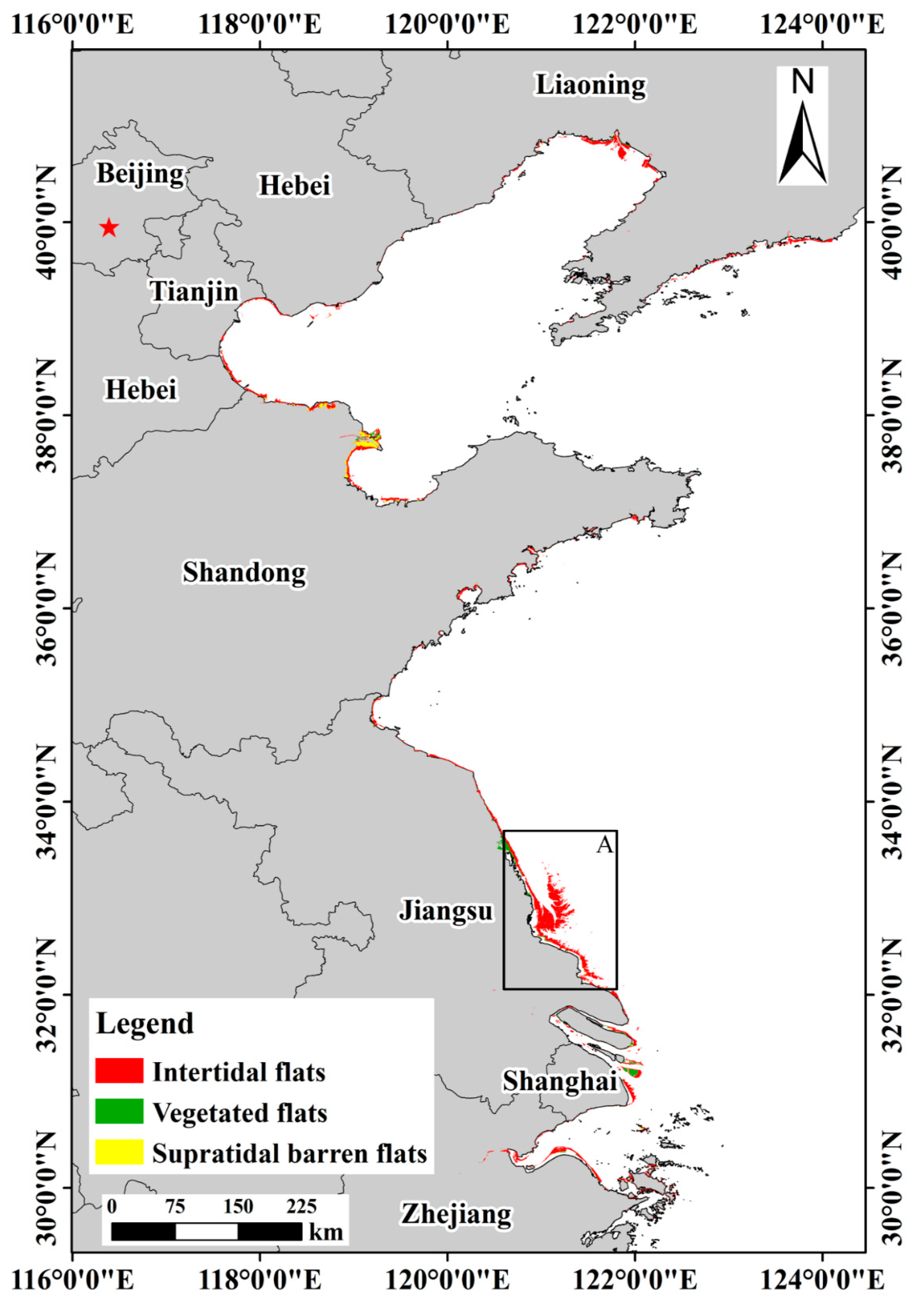
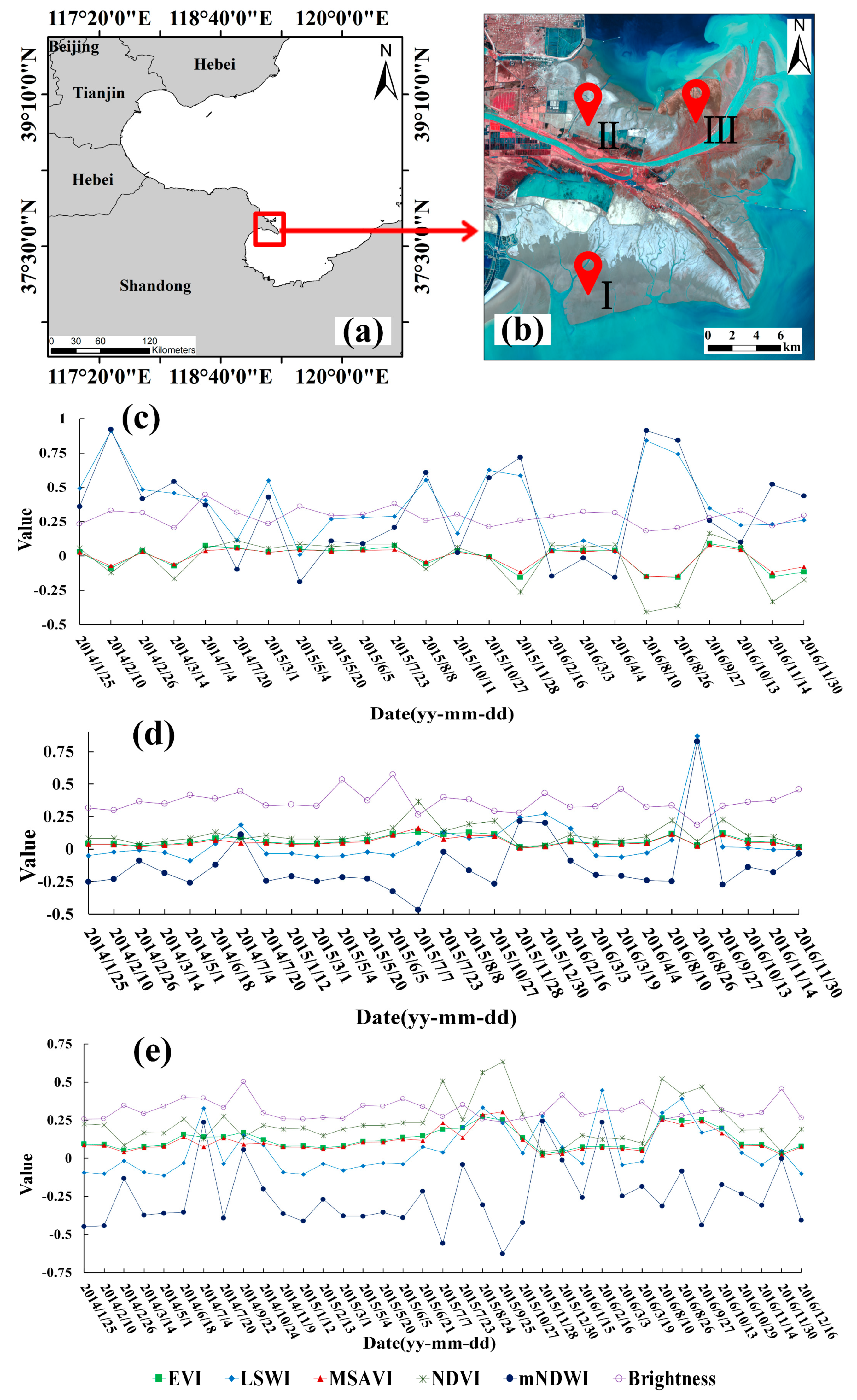
2.1. Study Area
2.2. Satellite Imagery and Auxiliary Data
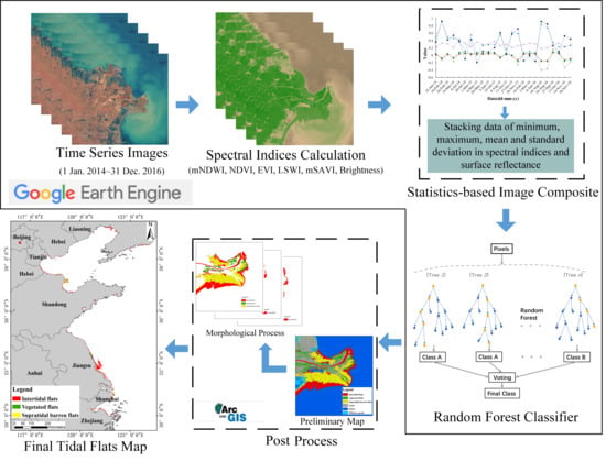
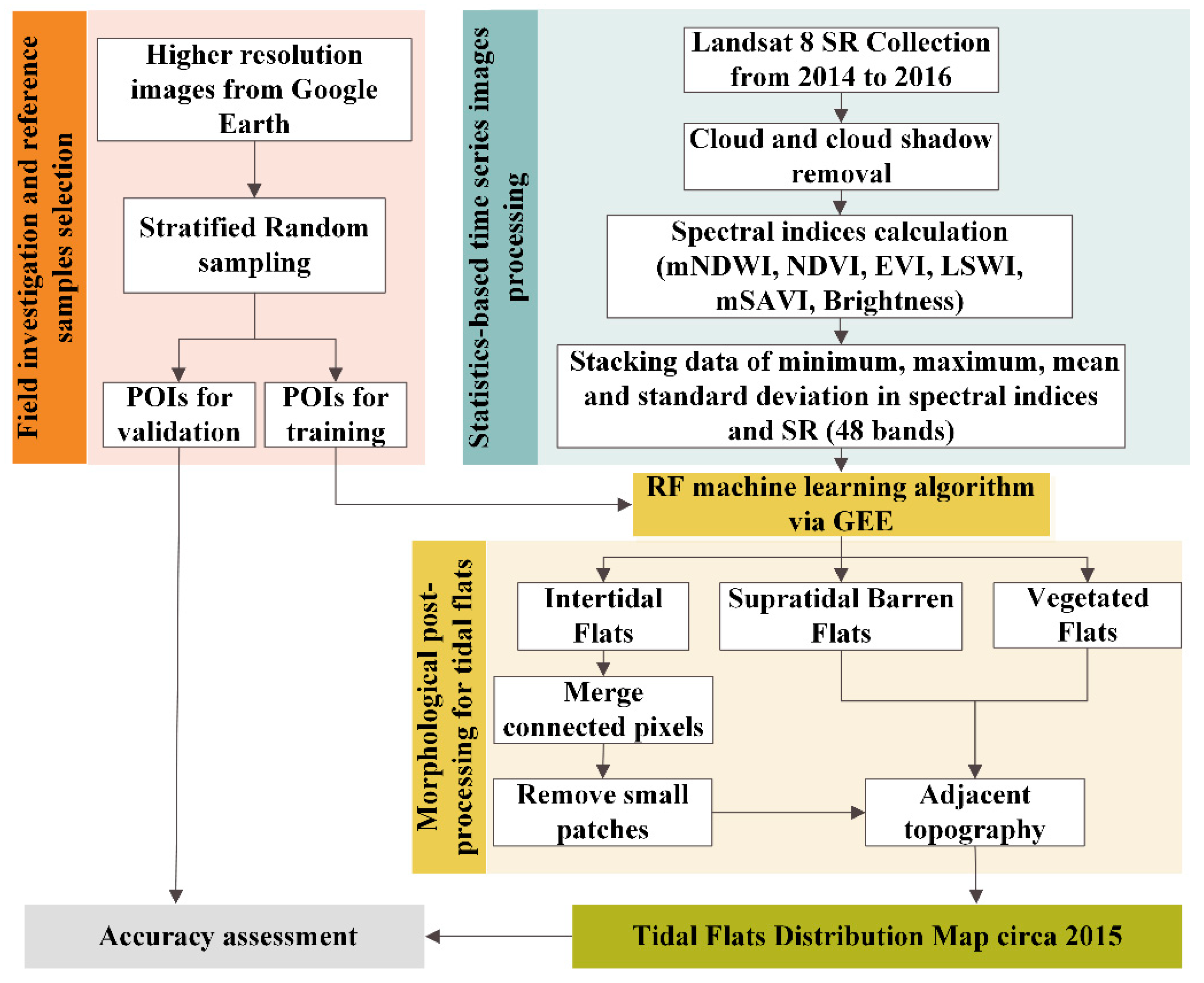
2.3. Methods
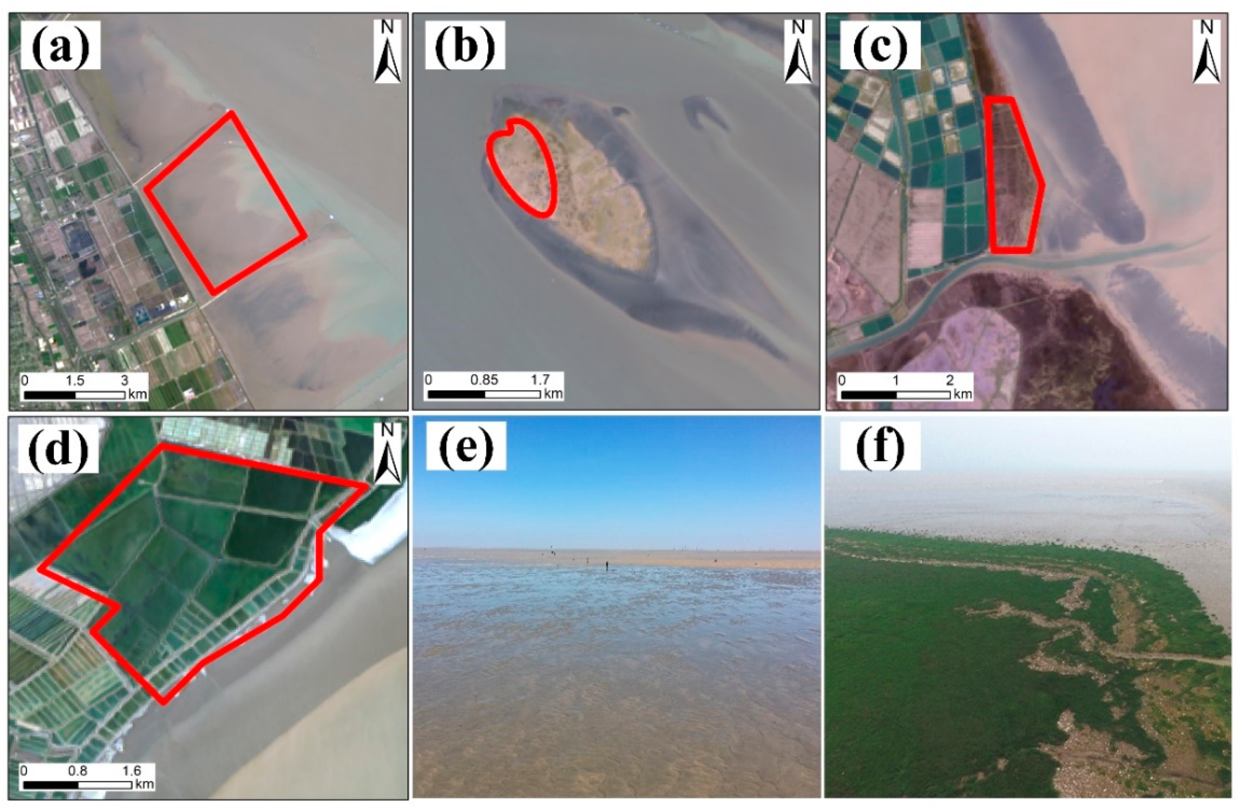
2.3.1. Field Investigation and Reference Sample Selection
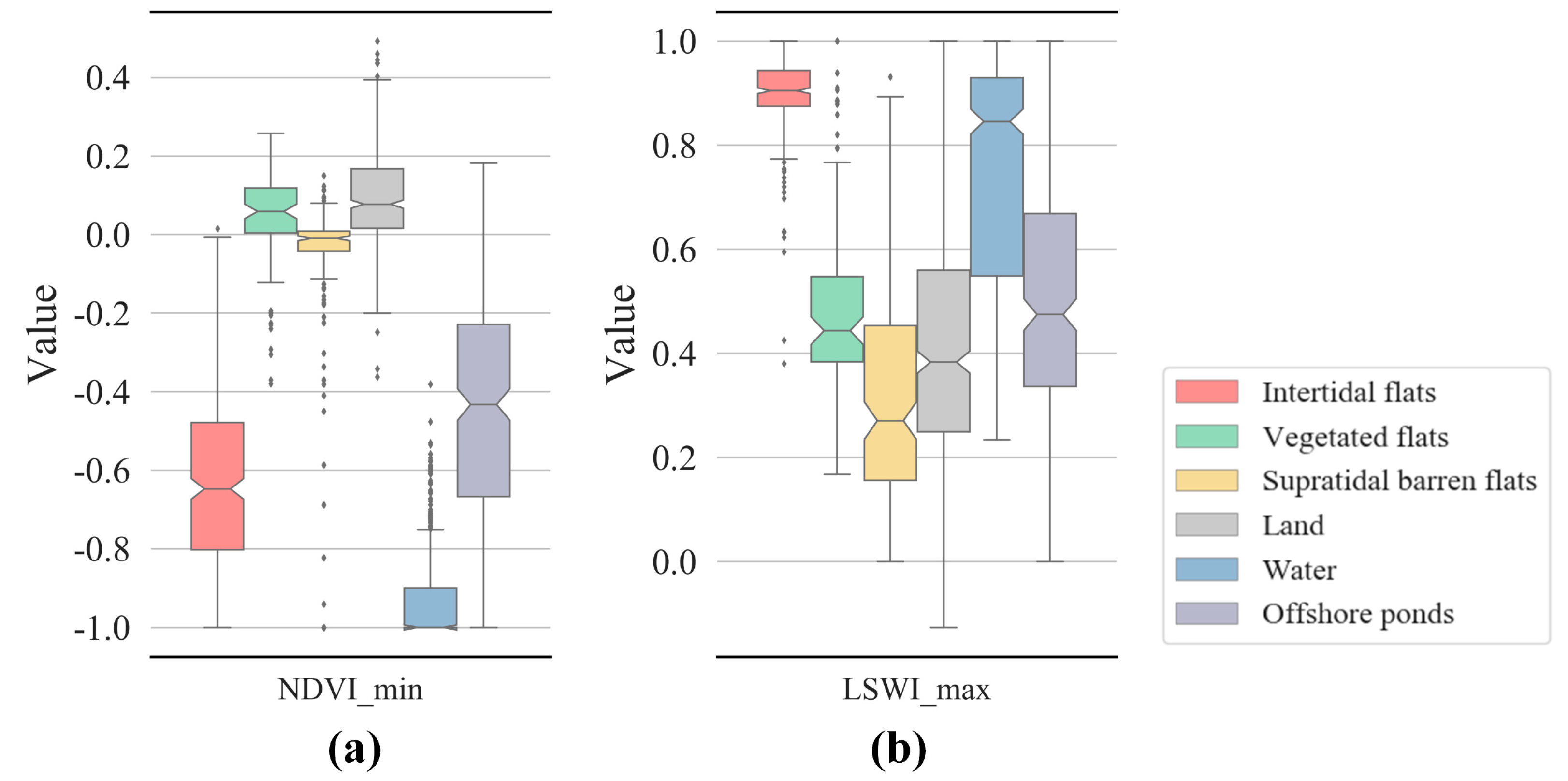
2.3.2. Statistics-Based Time-Series Images Processing
2.3.3. Random Forest (RF) Machine Learning Algorithm via Google Earth Engine (GEE)
2.3.4. Morphological Post-Processing for Tidal Flats
2.3.5. Accuracy Assessment
3. Results and Discussion
3.1. Tidal Flat Map
3.2. Extensive Tidal Flats towards Land
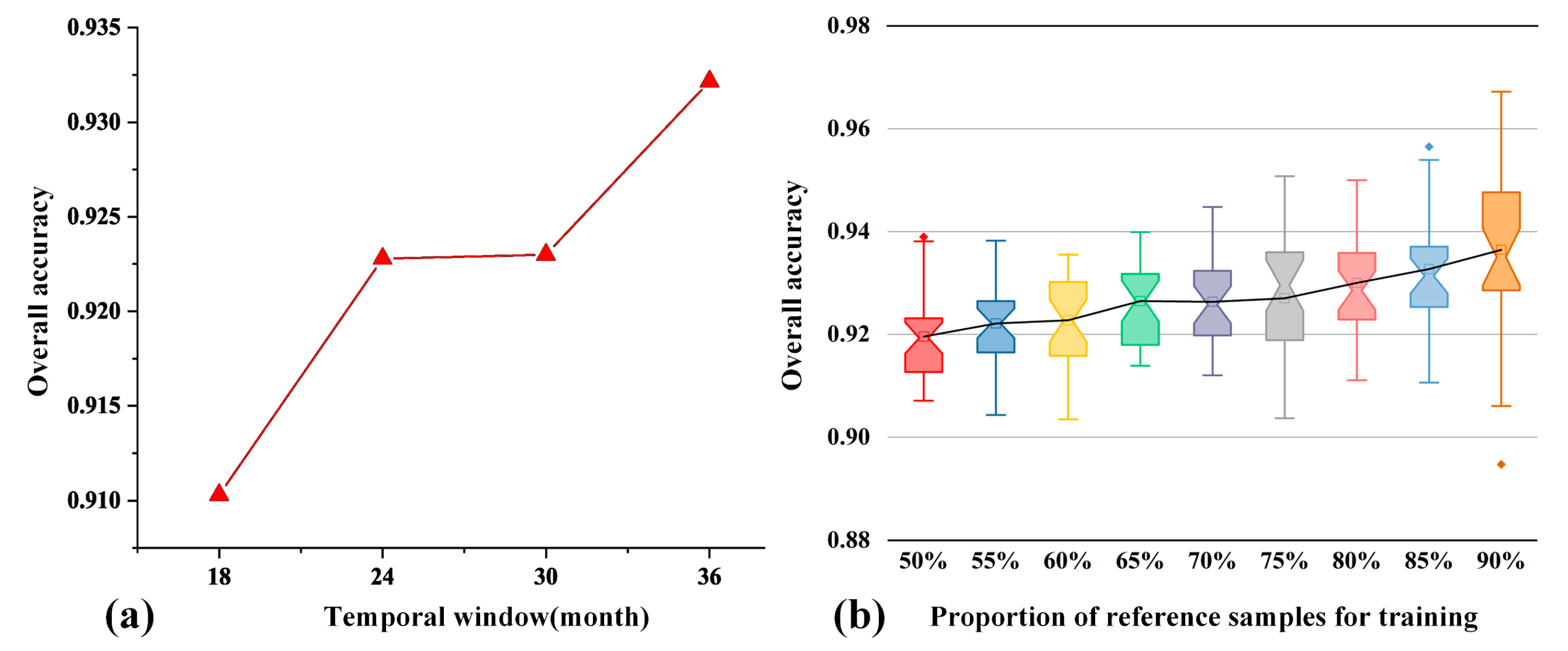
3.3. Sensitive Testing of Temporal Window and Training Samples
3.4. Comparison with Other Available Tidal Flat Maps
3.5. Limitation and Potential of GEE Cloud Platform for Tidal Flats Mapping
4. Conclusions
Author Contributions
Funding
Acknowledgments
Conflicts of Interest
References
- Healy, T.; Wang, Y. Integrated Coastal Zone Management for Sustainable Development—with Comment on ICZM Applicability to Muddy Coasts. J. Coast. Res. 2004, 229–242. [Google Scholar]
- Wang, Y.; Zhu, D.; Wu, X. Chapter Thirteen Tidal Flats and Associated Muddy Coast of China. In Proceedings in Marine Science; Healy, T., Wang, Y., Healy, J.A., Eds.; Elsevier: Amsterdam, The Netherlands, 2002; Volume 4, pp. 319–345. [Google Scholar]
- Small, C.; Nicholls, R.J. A Global Analysis of Human Settlement in Coastal Zones. J. Coast. Res. 2003, 19, 584–599. [Google Scholar]
- Murray, N.J.; Clemens, R.S.; Phinn, S.R.; Possingham, H.P.; Fuller, R.A. Tracking the Rapid Loss of Tidal Wetlands in the Yellow Sea. Front. Ecol. Environ. 2014, 12, 267–272. [Google Scholar] [CrossRef]
- Yang, B.; Wang, Y.; Zhu, D. The Tidal Flat Resources of China. J. Nat. Resour. 1997, 12, 307–316. [Google Scholar]
- Zhao, B.; Yan, Y.; Guo, H.; He, M.; Gu, Y.; Li, B. Monitoring Rapid Vegetation Succession in Estuarine Wetland Using Time Series Modis-Based Indicators: An Application in the Yangtze River Delta Area. Ecol. Indic. 2009, 9, 346–356. [Google Scholar] [CrossRef]
- Reineck, H.-E.; Singh, I.B. Tidal Flats. In Depositional Sedimentary Environments; Springer: Berlin/Heidelberg, Germany, 1980; pp. 430–456. [Google Scholar]
- Zhu, D.; Xu, T. The Coast Development and Exploitation of Middle Part of Jiangsu Coast. J. Nanjing Univ. (Nat. Sci.) 1982, 18, 799–818. [Google Scholar]
- Wang, X.; Xiao, X.; Zou, Z.; Chen, B.; Ma, J.; Dong, J.; Doughty, R.B.; Zhong, Q.; Qin, Y.; Dai, S. Tracking Annual Changes of Coastal Tidal Flats in China During 1986–2016 through Analyses of Landsat Images with Google Earth Engine. Remote Sens. Environ. 2018, in press. [Google Scholar] [CrossRef]
- Rogers, K.; Woodroffe, C.D. Tidal Flats and Salt Marshes. In Coastal Environments and Global Change; Masselink, G., Gehrels, R., Eds.; Wiley: New York, NY, USA, 2015; pp. 227–250. [Google Scholar]
- Li, J.; Lei, Y.; Cui, L.; Pan, X.; Zhang, X.; Zhang, M.; Li, W. Current Status and Research Progress of Coastal Tidal Flat Wetlands in China. For. Resour. Manag. 2018, 2, 24–28. [Google Scholar]
- Murray, N.J.; Phinn, S.R.; Clemens, R.S.; Roelfsema, C.M.; Fuller, R.A. Continental Scale Mapping of Tidal Flats across East Asia Using the Landsat Archive. Remote Sens. 2012, 4, 3417–3426. [Google Scholar] [CrossRef]
- Sun, X.; Teng, H.; Zhao, J.; Wang, Y.; Zhang, L.; Ye, Q. Airborne Lidar Coast Topographic Measurement Technology and Its Application. Hydrogr. Surv. Charting 2017, 37, 70–78. [Google Scholar]
- Heygster, G.; Dannenberg, J.; Notholt, J. Topographic Mapping of the German Tidal Flats Analyzing SAR Images with the Waterline Method. IEEE Trans. Geosci. Remote Sens. 2010, 48, 1019–1030. [Google Scholar] [CrossRef]
- McCarthy, M.J.; Radabaugh, K.R.; Moyer, R.P.; Muller-Karger, F.E. Enabling Efficient, Large-Scale High-Spatial Resolution Wetland Mapping Using Satellites. Remote Sens. Environ. 2018, 208, 189–201. [Google Scholar] [CrossRef]
- Tang, Z.; Li, Y.; Gu, Y.; Jiang, W.; Xue, Y.; Hu, Q.; LaGrange, T.; Bishop, A.; Drahota, J.; Li, R. Assessing Nebraska Playa Wetland Inundation Status During 1985–2015 Using Landsat Data and Google Earth Engine. Environ. Monit. Assess. 2016, 188, 654. [Google Scholar] [CrossRef]
- Li, S.; Liu, Z.; He, G.; Xia, D.; Wei, H. An Application System of Remote Sensing Imagery Interpretation for Tianjin Coast Area. Hydrogr. Surv. Charting 2005, 25, 13–15. [Google Scholar]
- Zhang, Z.; Wang, X.; Zhao, X.; Liu, B.; Yi, L.; Zuo, L.; Wen, Q.; Liu, F.; Xu, J.; Hu, S. A 2010 Update of National Land Use/Cover Database of China at 1: 100000 Scale Using Medium Spatial Resolution Satellite Images. Remote Sens. Environ. 2014, 149, 142–154. [Google Scholar] [CrossRef]
- Zhao, L.; Meng, L.; Zhang, Y.; Feng, W.; Zhang, J. Research on Joint Spectral and Texture Features SVM Tidal Classification and Extraction Algorithm. Eng. Surv. Mapp. 2016, 25, 43–46. [Google Scholar]
- Wang, C.; Liu, H.Y.; Zhang, Y.; Li, Y.F. Classification of Land-Cover Types in Muddy Tidal Flat Wetlands Using Remote Sensing Data. J. Appl. Remote Sens. 2014, 7, 073457. [Google Scholar] [CrossRef]
- Murray, N.J.; Phinn, S.R.; DeWitt, M.; Ferrari, R.; Johnston, R.; Lyons, M.B.; Clinton, N.; Thau, D.; Fuller, R.A. The Global Distribution and Trajectory of Tidal Flats. Nature 2018. [Google Scholar] [CrossRef]
- Whyte, A.; Ferentinos, K.P.; Petropoulos, G.P. A New Synergistic Approach for Monitoring Wetlands Using Sentinels-1 and 2 Data with Object-Based Machine Learning Algorithms. Environ. Model. Softw. 2018, 104, 40–54. [Google Scholar] [CrossRef]
- Ryu, J.H.; Won, J.S.; Min, K.D. Waterline Extraction from Landsat Tm Data in a Tidal Flat: A Case Study in Gomso Bay, Korea. Remote Sens. Environ. 2002, 83, 442–456. [Google Scholar] [CrossRef]
- Tseng, K.H.; Kuo, C.Y.; Lin, T.H.; Huang, Z.C.; Lin, Y.C.; Liao, W.H.; Chen, C.F. Reconstruction of Time-Varying Tidal Flat Topography Using Optical Remote Sensing Imageries. ISPRS J. Photogramm. Remote Sens. 2017, 131, 92–103. [Google Scholar] [CrossRef]
- Liu, X.; Gao, Z.; Ning, J.; Yu, X.; Zhang, Y. An Improved Method for Mapping Tidal Flats Based on Remote Sensing Waterlines: A Case Study in the Bohai Rim, China. IEEE J. Sel. Top. Appl. Earth Obs. Remote Sens. 2016, 9, 5123–5129. [Google Scholar]
- Ryu, J.H.; Kim, C.H.; Lee, Y.K.; Won, J.S.; Chun, S.S.; Lee, S. Detecting the Intertidal Morphologic Change Using Satellite Data. Estuar. Coast. Shelf Sci. 2008, 78, 623–632. [Google Scholar] [CrossRef]
- Liu, Y.; Li, M.; Zhou, M.; Yang, K.; Mao, L. Quantitative Analysis of the Waterline Method for Topographical Mapping of Tidal Flats: A Case Study in the Dongsha Sandbank, China. Remote Sens. 2013, 5, 6138–6158. [Google Scholar] [CrossRef]
- Sagar, S.; Roberts, D.; Bala, B.; Lymburner, L. Extracting the Intertidal Extent and Topography of the Australian Coastline from a 28 Year Time Series of Landsat Observations. Remote Sens. Environ. 2017, 195, 153–169. [Google Scholar] [CrossRef]
- Chen, B.; Xiao, X.; Li, X.; Pan, L.; Doughty, R.; Ma, J.; Dong, J.; Qin, Y.; Zhao, B.; Wu, Z. A Mangrove Forest Map of China in 2015: Analysis of Time Series Landsat 7/8 and Sentinel-1a Imagery in Google Earth Engine Cloud Computing Platform. ISPRS J. Photogramm. Remote Sens. 2017, 131, 104–120. [Google Scholar] [CrossRef]
- Dong, J.; Xiao, X.; Menarguez, M.A.; Zhang, G.; Qin, Y.; Thau, D.; Biradar, C.; Moore, B., III. Mapping Paddy Rice Planting Area in Northeastern Asia with Landsat 8 Images, Phenology-Based Algorithm and Google Earth Engine. Remote Sens. Environ. 2016, 185, 142–154. [Google Scholar] [CrossRef]
- Teluguntla, P.; Thenkabail, P.; Oliphant, A.; Xiong, J.; Gumma, M.K.; Congalton, R.G.; Yadav, K.; Huete, A. A 30-M Landsat-Derived Cropland Extent Product of Australia and China Using Random Forest Machine Learning Algorithm on Google Earth Engine Cloud Computing Platform. ISPRS J. Photogramm. Remote Sens. 2018, 144, 325–340. [Google Scholar] [CrossRef]
- Dong, J.; Xiao, X.; Chen, B.; Torbick, N.; Jin, C.; Zhang, G.; Biradar, C. Mapping Deciduous Rubber Plantations through Integration of PALSAR and Multi-Temporal Landsat Imagery. Remote Sens. Environ. 2013, 134, 392–402. [Google Scholar] [CrossRef]
- Hird, J.N.; DeLancey, E.R.; McDermid, G.J.; Kariyeva, J. Google Earth Engine, Open-Access Satellite Data, and Machine Learning in Support of Large-Area Probabilistic Wetland Mapping. Remote Sens. 2017, 9, 1315. [Google Scholar] [CrossRef]
- Gorelick, N.; Hancher, M.; Dixon, M.; Ilyushchenko, S.; Thau, D.; Moore, R. Google Earth Engine: Planetary-Scale Geospatial Analysis for Everyone. Remote Sens. Environ. 2017, 202, 18–27. [Google Scholar] [CrossRef]
- Zhao, X. Wetlands: Homeland for Harmonious Coexistence of Man and Nature; China Forestry Press: Beijing, China, 2005. [Google Scholar]
- Su, S. Overview on the Seven-Year National Multipurpose Investigation of the Coastal Zone and Tidal Wetland Resources. Ocean Coast. -Zone Dev. 1988, 2, 30–32. [Google Scholar]
- National Bureau of Statistics of China. China Statistical Yearbook of 2015. Available online: http://www.stats.gov.cn/tjsj/ndsj/2015/indexeh.htm (accessed on 14 September 2018).
- USGS. Product Guide: Landsat 8 Surface Reflectance Code (LaSRC) Product. Available online: https://landsat.usgs.gov/sites/default/files/documents/lasrc_product_guide.pdf (accessed on 26 December 2018).
- Foga, S.; Scaramuzza, P.L.; Guo, S.; Zhu, Z.; Dilley, R.D.; Beckmann, T.; Schmidt, G.L.; Dwyer, J.L.; Hughes, M.J.; Laue, B. Cloud Detection Algorithm Comparison and Validation for Operational Landsat Data Products. Remote Sens. Environ. 2017, 194, 379–390. [Google Scholar] [CrossRef]
- Hijmans, R.; Garcia, N.; Kapoor, J.; Rala, A.; Maunahan, A.; Wieczorek, J. Global Administrative Areas (Boundaries); Berkeley: Museum of Vertebrate Zoology and the International Rice Research Institute, University of California: Berkeley, CA, USA, 2012. [Google Scholar]
- Wessel, P.; Smith, W.H. A Global, Self-Consistent, Hierarchical, High-Resolution Shoreline Database. J. Geophys. Res. Solid Earth 1996, 101, 8741–8743. [Google Scholar] [CrossRef]
- Hou, X.; Di, X.; Hou, W.; Wu, L. Accuracy Evaluation of Land Use Mapping Using Remote Sensing Techniques in Coastal Zone of China. J. Geo-Inf. Sci. 2018, 20, 1478–1488. [Google Scholar]
- Zhan, Y.; Zhu, Y.; Su, Y.; Cui, Y. Eco-Environmental Changes in Yancheng Coastal Zone Based on the Domestic Resource Satellite Data. Remote Sens. Land Resour. 2017, 29, 160–165. [Google Scholar]
- Di, X.; Hou, X.; Wu, L. Land Use Classification System for China’s Coastal Zone Based on Remote Sensing. Resour. Sci. 2014, 36, 463–472. [Google Scholar]
- Shao, W.; Li, G.; Wang, L.; Dong, L.; Qi, F.; Ma, L. Changes of Tidal Flat and Coastline in the Northern Shandong Peninsula in Recent 30 Years. J. Appl. Oceanogr. 2017, 36, 512–518. [Google Scholar]
- Fan, D.; Wang, Y.; Liu, M. Classifications, Sedimentary Features and Facies Associations of Tidal Flats. J. Palaeogeogr. 2013, 2, 66–80. [Google Scholar]
- European Environment Agency. CORINE Land Cover. Available online: https://www.eea.europa.eu/publications/COR0-landcover (accessed on 12 October 2018).
- Xu, H. Modification of Normalised Difference Water Index (NDWI) to Enhance Open Water Features in Remotely Sensed Imagery. Int. J. Remote Sens. 2006, 27, 3025–3033. [Google Scholar] [CrossRef]
- Tucker, C.J. Red and Photographic Infrared Linear Combinations for Monitoring Vegetation. Remote Sens. Environ. 1979, 8, 127–150. [Google Scholar] [CrossRef]
- Xiao, X.M.; Hollinger, D.; Aber, J.; Goltz, M.; Davidson, E.A.; Zhang, Q.Y.; Moore, B. Satellite-Based Modeling of Gross Primary Production in an Evergreen Needleleaf Forest. Remote Sens. Environ. 2004, 89, 519–534. [Google Scholar] [CrossRef]
- Qi, J.; Chehbouni, A.; Huete, A.R.; Kerr, Y.H.; Sorooshian, S. A Modified Soil Adjusted Vegetation Index. Remote Sens. Environ. 1994, 48, 119–126. [Google Scholar] [CrossRef]
- Huete, A.; Didan, K.; Miura, T.; Rodriguez, E.P.; Gao, X.; Ferreira, L.G. Overview of the Radiometric and Biophysical Performance of the Modis Vegetation Indices. Remote Sens. Environ. 2002, 83, 195–213. [Google Scholar] [CrossRef]
- Baig, M.H.A.; Zhang, L.; Shuai, T.; Tong, Q. Derivation of a Tasselled Cap Transformation Based on Landsat 8 at-Satellite Reflectance. Remote Sens. Lett. 2014, 5, 423–431. [Google Scholar] [CrossRef]
- Pal, M. Random Forest Classifier for Remote Sensing Classification. Int. J. Remote Sens. 2005, 26, 217–222. [Google Scholar] [CrossRef]
- Hawbaker, T.J.; Vanderhoof, M.K.; Beal, Y.J.; Takacs, J.D.; Schmidt, G.L.; Falgout, J.T.; Williams, B.; Fairaux, N.M.; Caldwell, M.K.; Picotte, J.J. Mapping Burned Areas Using Dense Time-Series of Landsat Data. Remote Sens. Environ. 2017, 198, 504–522. [Google Scholar] [CrossRef]
- Stroppiana, D.; Bordogna, G.; Carrara, P.; Boschetti, M.; Boschetti, L.; Brivio, P. A Method for Extracting Burned Areas from Landsat TM/ETM+ Images by Soft Aggregation of Multiple Spectral Indices and a Region Growing Algorithm. ISPRS J. Photogramm. Remote Sens. 2012, 69, 88–102. [Google Scholar] [CrossRef]
- Chen, J.; Liao, A.; Chen, J.; Peng, S.; Chen, L.; Zhang, H. 30-Meter Globalland Cover Data Product-Globeland30. Geomat. World 2017, 24, 1–8. [Google Scholar]
- Kang, Y.; Ding, X.; Xu, F.; Zhang, C.; Ge, X. Topographic Mapping on Large-scale Tidal Flats with an Iterative Approach on the Waterline Method. Estuar. Coast. Shelf Sci. 2017, 190, 11–22. [Google Scholar] [CrossRef]
- Liu, Y.; Zhang, R.; Li, M. Study of the Remote Sensing Extraction Method of Ground Object Information on the Jiangsu Tidal Flat. Adv. Mar. Sci. 2004, 22, 210–214. [Google Scholar]
- Dhanjal-Adams, K.L.; Hanson, J.O.; Murray, N.J.; Phinn, S.R.; Wingate, V.R.; Mustin, K.; Lee, J.R.; Allan, J.R.; Cappadonna, J.L.; Studds, C.E. The Distribution and Protection of Intertidal Habitats in Australia. Emu-Austral Ornithol. 2016, 116, 208–214. [Google Scholar] [CrossRef]
- Ravanelli, R.; Nascetti, A.; Cirigliano, R.V.; Di Rico, C.; Leuzzi, G.; Monti, P.; Crespi, M. Monitoring the Impact of Land Cover Change on Surface Urban Heat Island through Google Earth Engine: Proposal of a Global Methodology, First Applications and Problems. Remote Sens. 2018, 10, 1488. [Google Scholar] [CrossRef]


| Class | Description | Reference Samples |
|---|---|---|
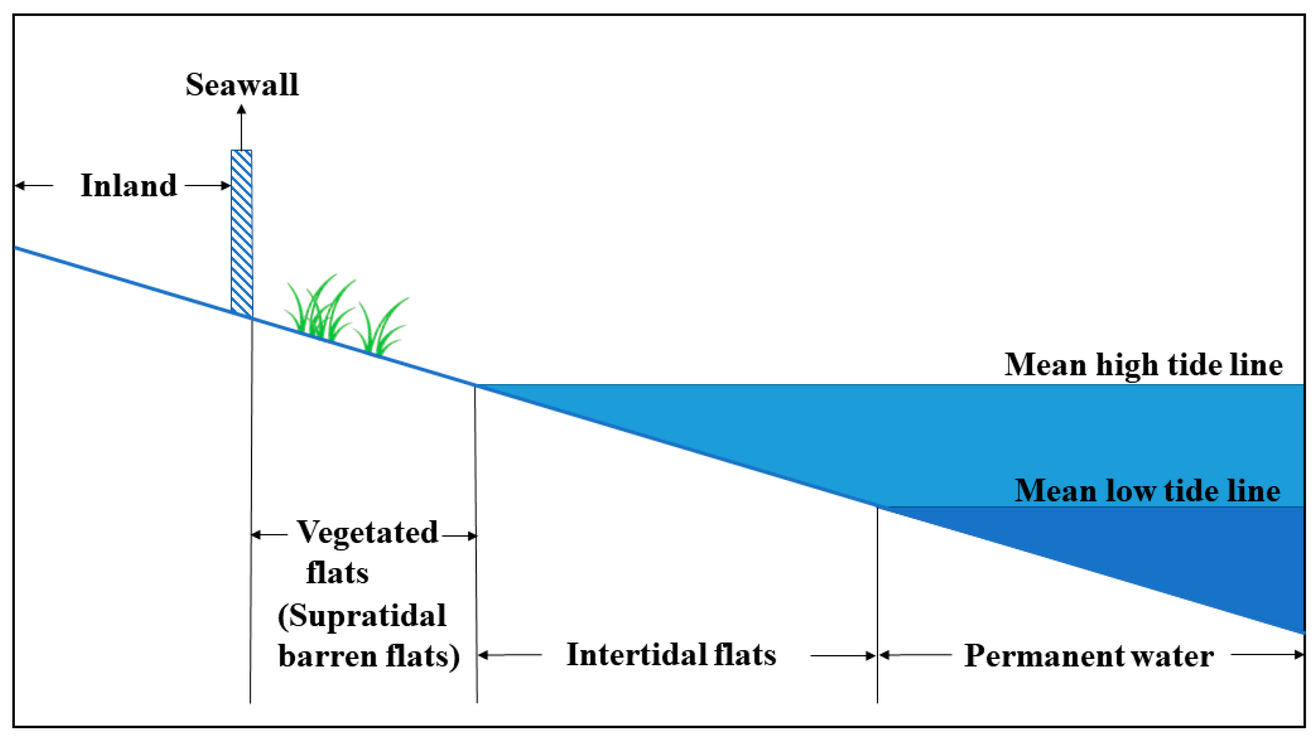
| Intertidal Flats | Tidal flats located between mean high tide line and mean low tide line | 377 |
| Supratidal Barren Flats | Tidal flats located above mean high tide line and outside the artificial borders | 166 |
| Vegetated Flats | Tidal flats covered with coastal vegetation and outside the artificial borders | 92 |
| Land | Urban areas, cropland, forests and artificial coastal construction | 529 |
| Water | Permanent water | 616 |
| Offshore Ponds | Agriculture ponds and saline | 296 |
| Total | - | 2076 |
| Reference | Intertidal Flats | Vegetated Flats | Supratidal Barren Flats | Others | Total | User’s (%) | |
|---|---|---|---|---|---|---|---|
| Classified | |||||||
| Intertidal flats | 86 | 0 | 0 | 2 | 88 | 97.7 | |
| Vegetated flats | 0 | 18 | 0 | 1 | 19 | 94.7 | |
| Supratidal barren flats | 2 | 0 | 30 | 0 | 32 | 93.8 | |
| Others | 1 | 5 | 5 | 293 | 304 | 96.4 | |
| Total | 89 | 23 | 35 | 296 | 443 | ||
| Producer’s (%) | 96.6 | 78.3 | 85.7 | 96.2 | |||
| Overall accuracy (%) | 94.4 | ||||||
| Region | Tidal Flats Area(km2) | Total | ||
|---|---|---|---|---|
| Intertidal Flats | Supratidal Barren Flats | Vegetated Flats | ||
| Zhejiang | 407.95 | 10.10 | 15.84 | 433.89 |
| Shanghai | 343.01 | 7.94 | 124.74 | 475.69 |
| Jiangsu | 1767.56 | 6.57 | 168.20 | 1942.33 |
| Shandong | 619.53 | 259.52 | 42.58 | 921.63 |
| Tianjin | 44.14 | 0.78 | 2.25 | 47.17 |
| Hebei | 155.61 | 6.35 | 0.03 | 161.99 |
| Liaoning | 622.10 | 2.27 | 22.60 | 646.97 |
| Total | 3959.90 | 293.53 | 376.24 | 4629.67 |
| Coastal Provincial Region | Coastal City | Tidal Flats (Intertidal Flats) Area(km2) | Identical Area(km2) | |||
|---|---|---|---|---|---|---|
| LUCC 2015 | Murry’s | Proposed | LUCC 2015 vs. Proposed | Murray’s vs. Proposed | ||
| Zhejiang | Hangzhou | 0.36 | 54.00 | 30.63 | 0 | 21.66(70.7%) |
| Ningbo | 43.37 | 346.32 | 191.89 | 0.43(0.2%) | 168.05(87.6%) | |
| Jiaxing | 13.64 | 67.76 | 72.22 | 9.84(13.6%) | 52.30(72.4%) | |
| Shaoxing | 0.37 | 51.65 | 5.77 | 0 | 3.85(66.7%) | |
| Zhoushan | 39.09 | 140.75 | 107.43 | 0.24(0.2%) | 36.51(34.0%) | |
| Shanghai | Shanghai | 92.8 | 412.88 | 343.66 | 5.88(1.7%) | 278.82(81.1%) |
| Jiangsu | Nantong | 531.21 | 660.79 | 453.23 | 274.5(60.6%) | 412.61(91.0%) |
| Lianyungang | 2.89 | 255.71 | 62.68 | 0.07(0.1%) | 53.01(84.6%) | |
| Yancheng | 441.02 | 2036.98 | 1249.25 | 265.78(21.3%) | 1125.62(90.1%) | |
| Shandong | Qingdao | 114.81 | 200.70 | 97.92 | 50.17(51.2%) | 85.44(87.2%) |
| Dongying | 358.57 | 558.97 | 289.81 | 132.59(45.8%) | 232.23(80.1%) | |
| Yantai | 119.37 | 180.71 | 37.01 | 18.66(50.4%) | 32.30(87.3%) | |
| Weifang | 211.48 | 222.18 | 79.61 | 61.53(77.3%) | 77.49(97.3%) | |
| Weihai | 34.68 | 159.98 | 42.45 | 0.39(0.9%) | 34.84(82.1%) | |
| Rizhao | 24.59 | 41.34 | 7.92 | 7.61(96.1%) | 7.64(96.5%) | |
| Binzhou | 20.05 | 153.59 | 64.81 | 2.78(4.3%) | 63.42(97.8%) | |
| Tianjin | Tianjin | 123.25 | 178.89 | 44.14 | 41.97(95.1%) | 41.45(93.9%) |
| Hebei | Tangshan | 155.84 | 303.18 | 78.58 | 54.96(69.9%) | 75.61(96.2%) |
| Cangzhou | 22.59 | 221.01 | 68.76 | 2.92(4.2%) | 66.84(97.2%) | |
| Qinhuangdao | 8.39 | 25.96 | 8.27 | 1.51(18.2%) | 1.11(13.4%) | |
| Liaoning | Dalian | 28.83 | 393.99 | 116.48 | 0.35(0.3%) | 83.78(71.9%) |
| Dandong | 4.96 | 233.54 | 108.76 | 0 | 102.56(94.3%) | |
| Jinzhou | 68.14 | 178.96 | 57.04 | 18.43(32.3%) | 49.94 (87.6%) | |
| Liaoning | Yingkou | 0.74 | 143.54 | 83.55 | 0.03(0.04%) | 79.26(94.9%) |
| Panjin | 135.47 | 299.48 | 213.71 | 28.26(13.2%) | 199.03(93.1%) | |
| Huludao | 44.36 | 76.48 | 42.55 | 3.33(7.8%) | 33.73(79.3%) | |
| Total | - | 2640.87 | 7599.34 | 3958.13 | 982.23(24.8%) | 3419.10(86.4%) |
© 2019 by the authors. Licensee MDPI, Basel, Switzerland. This article is an open access article distributed under the terms and conditions of the Creative Commons Attribution (CC BY) license (http://creativecommons.org/licenses/by/4.0/).
Share and Cite
Zhang, K.; Dong, X.; Liu, Z.; Gao, W.; Hu, Z.; Wu, G. Mapping Tidal Flats with Landsat 8 Images and Google Earth Engine: A Case Study of the China’s Eastern Coastal Zone circa 2015. Remote Sens. 2019, 11, 924. https://doi.org/10.3390/rs11080924
Zhang K, Dong X, Liu Z, Gao W, Hu Z, Wu G. Mapping Tidal Flats with Landsat 8 Images and Google Earth Engine: A Case Study of the China’s Eastern Coastal Zone circa 2015. Remote Sensing. 2019; 11(8):924. https://doi.org/10.3390/rs11080924
Chicago/Turabian StyleZhang, Kangyong, Xuanyan Dong, Zhigang Liu, Wenxiu Gao, Zhongwen Hu, and Guofeng Wu. 2019. "Mapping Tidal Flats with Landsat 8 Images and Google Earth Engine: A Case Study of the China’s Eastern Coastal Zone circa 2015" Remote Sensing 11, no. 8: 924. https://doi.org/10.3390/rs11080924
APA StyleZhang, K., Dong, X., Liu, Z., Gao, W., Hu, Z., & Wu, G. (2019). Mapping Tidal Flats with Landsat 8 Images and Google Earth Engine: A Case Study of the China’s Eastern Coastal Zone circa 2015. Remote Sensing, 11(8), 924. https://doi.org/10.3390/rs11080924