Ionospheric Rayleigh Wave Disturbances Following the 2018 Alaska Earthquake from GPS Observations

Abstract

Big earthquakes often excite the acoustic resonance between the earth’s surface and the lower atmosphere. The perturbations can propagate upward into the ionosphere and trigger ionospheric anomalies detected by dual-frequency GPS observations, but coseismic ionospheric disturbance (CID) directivity and mechanism are not clear. In this paper, the ionospheric response to the Mw = 7.9 Alaska earthquake on 23 January 2018 is investigated from about 100 continuous GPS stations near the epicenter. The fourth-order zero-phase Butterworth band-pass filter with cutoffs of 2.2 mHz and 8 mHz is applied to obtain the ionospheric disturbances. Results show that the CIDs with an amplitude of up to 0.06 total electron content units (TECU) are detected about 10 min after the Alaska earthquake. The CIDs are as a result of the upward propagation acoustic waves triggered by the Rayleigh wave. The propagation velocities of TEC disturbances are around 2.6 km/s, which agree well with the wave propagation speed of 2.7 km/s detected by the bottom pressure records. Furthermore, the ionospheric disturbances following the 2018 Mw = 7.9 Alaska earthquake are inhomogeneous and directional which is rarely discussed. The magnitude of ionospheric disturbances in the western part of the epicenter is more obvious than in the eastern part. This phenomenon also corresponds to the data obtained from the seismographs and bottom pressure records (BPRs) at the eastern and western side of the epicenter.

1. Introduction

During a major earthquake, the ground motion can provoke the acoustic resonance between the atmosphere and Earth’s surface. These resonances propagating into the ionosphere can cause oscillations in the ionosphere such as electron density (Ne) and total electron content (TEC). Studies on the acoustic resonance after earthquakes can provide insights on lithosphere-atmosphere-ionosphere coupling and ionospheric anomaly behaviors. The disturbance propagated from the epicenter area after the great Mw = 9.2 Alaska earthquake in 1964 was firstly detected by ionospheric vertical sounding [1]. Later the analysis of the seismic ionospheric disturbance characteristics provided a new opportunity on earthquake study. Due to the limitation of spatial coverage and resolution of traditional ionospheric monitoring methods [2,3], it is difficult to understand well the seismic ionospheric disturbance morphology and the coupling processes between the ground motion and ionospheric dynamics comprehensively.

Since the seismic ionospheric anomalies were first observed through GPS TEC in the California Northridge earthquake in 1994 [4], a number of studies have been conducted to study coseismic ionospheric disturbances (CIDs) associated with earthquakes. With the increase of continuously operating GPS stations, it provides not only plentiful observations to monitor the pattern and evolution of ionospheric disturbances, but also a great chance to study more details about the coupling between the solid-Earth and atmosphere. The energy released by the earthquake affects the atmosphere in the form of waves of seismic vertical deformation and earthquake-induced tsunami [5,6,7]. Due to the attenuation of atmospheric density, ionospheric disturbances are significantly amplified during the propagation from the ground to the ionosphere [8]. Ground motion in millimeters per second may cause neutral atmospheric disturbances of a few hundred meters at the ionospheric height [9,10]. Different methods are used to study the propagation speed of CIDs and find the source location [6,11,12,13]. Earthquakes provide unique possibilities to study the response of the ionosphere to earthquakes and better understand the coupling between the solid earth, troposphere, and ionosphere. Strong N-shaped waves following the 2008 Wenchuan earthquake with a plane waveform was found [14]. In the March 2011 earthquake in Japan, dense TEC disturbances clearly indicated the existence of acoustic-gravity waves generated above the epicenter, the acoustic waves coupled with the Rayleigh waves, and the gravity waves combined with the subsequent tsunami propagation [6,15]. High-frequency signals of 3.83 mHz and 5.83 mHz in TEC variations exist only near the epicenter area, which is probably due to attenuation of interference propagation [6]. Multi-segment structures of seismic faults were detected from high-speed ionospheric GPS data [16,17]. The 2012 Mw = 7.8 Haida Gwaii earthquake analyzed and discussed the CIDs propagation characteristics and direction divergence, as well as the correlation and coupling between ionospheric disturbances and ground vertical motion [18]. Jin [19] used Plate Boundary Observatory (PBO) GPS observations around the 2005 Northern California offshore earthquake to observe the ionospheric disturbances induced by the earthquake. The southward CIDs following 2015 Mw 7.8 Gorkha, Nepal Earthquake were found to propagate to the F2 region with ~300–440 km captured by COSMIC radio occultation observations [20,21].

However, the disturbance directivity and mechanism of the solid, troposphere, and ionosphere coupling remain unclear. Normally, the vertical displacement of the seismic zone plays a more important role in the formation of seismic ionospheric disturbances [21]. Therefore, earthquakes dominated by strike-slip motion with very small vertical coseismic component are not expected to generate ionospheric perturbations. The relationship between seismic displacement and ionospheric changes has not been fully understood so far [8,22,23]. With no large vertical static coseismic crustal displacements, other seismological parameters such as the magnitude of coseismic horizontal displacements, dimensions of seismic faults and slips at the fault, or a combination of them, may play an important role [24]. In this paper, the ionospheric disturbances following the 2018 Alaska earthquake dominated by strike-slip motion are investigated from the near-field dense GPS observations and the focal mechanism solutions indicate faulting occurred on a steeply dipping fault striking either west-southwest or north-northwest [25]. This is the first study on the ionospheric disturbances after the 2018 Alaska earthquake. The data from four instruments were used to analyze the coseismic ionospheric disturbances. The propagation features and directional divergences are investigated and discussed as well as the correlation and coupling between the ionospheric disturbance and ground vertical movement. the regional difference of Rayleigh wave velocity was considered to be one of the important reasons for the diversity of the characteristics of the coseismic ionospheric propagation.

2. Data and Method

2.1. Earthquake and Data

The Alaska earthquake with the magnitude of Mw = 7.9 erupted at 9:31 UT on 23 January 2018. The epicenter (56.004°N, 149.166°W) was located at 280 km southeast of Kodiak, Alaska, with a focal depth of 14.1 km. Shortly after the strong earthquake, aftershocks of magnitude 4.7 and 5 occurred in the sea near Alaska. The curvature of the arc results in a westward transition of relative plate motion from trench-normal in the east to trench-parallel in the west, accompanied by westward variations in seismic activity. The Pacific plate subducts beneath the North America plate at the Alaska-Aleutians Trench. The largest earthquakes in this region are generally shallow, predominantly strike-slip events. The location and mechanism of the Alaska earthquakes are consistent with it occurring on a fault system within the Pacific plate before it subducts [25].

The GPS data used to calculate the GPS-TEC time series in our work was obtained from the University Navstar Consortium (UNAVCO) at ftp://data-out.unavco.org/pub. In addition, 91 Alaska’s broadband seismographs (BBS) were used to estimate the group velocity of surface Rayleigh wave propagation in different directions. In this study, only the z component data of the seismographs were used to observe the vertical displacement data. The data of seismographs can be obtained from IRIS (Incorporated Research Institutions for Seismology) at http://www.iris.edu. The ground vertical motion was detected by the bottom pressure records (BPRs) on Deep-ocean Assessment and Reporting of Tsunamis (DART) buoy to study the speed of the wave propagation on the sea surface. The data of BPRs can be obtained from NDBC (National Data Buoy Center) at https://www.ndbc.noaa.gov/. Ionospheric plasma electron densities obtained from Formosat-3/COSMIC on the day of the earthquake and two days before and after are also used. This data was obtained from http://cdaac-www.cosmic.ucar.edu. The locations of all stations mentioned above are shown in Figure 1.

2.2. Methods

Ionospheric delay in GPS satellite signals depends on the signal frequency and TEC on the propagation path. When only considering the frequency, it is inversely proportional to the square of the frequency f of the signals ($f_1=1575.42 \mathrm{MHz}$ and $f_2=1227.60 \mathrm{MHz}$). The time difference of the dual-frequency carrier phase and pseudorange observations contains the information of the ionospheric delay. When calculating TEC, it is assumed that all the electrons in the ionosphere are concentrated in a thin shell at a certain height which is called the single layer model (SLM). In this study, the ionosphere was assumed to be concentrated at a height of 280 km. This height is around the height of the peak determined by the electron density (Ne) profile above the Alaska area. Since the TEC changes with the change of signal elevation and azimuth angle, the ionospheric anomaly detection often focuses on the vertical TEC (VTEC). The TEC can be calculated by the following equation [6,18]:

$$STEC=\frac{f_1^2{f}_2^2}{40.3\left(f_1^2-f_2^2\right)}\left(L_1-L_2+{\lambda }_1\left(N_1+b_1\right)-{\lambda }_2\left(N_2+b_2\right)+{\epsilon }_L\right)$$

(1)

$$VTEC=STEC·\cos \left(\arcsin \left(\frac{R·\sin \left(z\right)}{R+H}\right)\right)$$

(2)

where STEC is the slant TEC, L is the carrier phase observation (meter), λ is the signal wavelength, N is the carrier phase integer ambiguity, b is the instrument biases for carrier phase, ${\epsilon }_L$ is the other residuals, R is the earth radius, H is the thin shell height of the ionosphere, and z is the satellite’s elevation angle. All TECs mentioned below refer to VTEC.

Before estimating STEC from GPS observations, the cycle slips and gross error in the carrier phase observation should be eliminated. The Second-order Time-difference Phase Ionospheric Residual (STPIR) was used to detect and repair the cycle slip [26]. The accuracy of the GPS carrier phase measurement is about 1 mm under ideal conditions, and therefore the error of TEC is about 0.01 TECU according to the law of propagation of error [6]. The TEC anomalies can be significantly detected when the detrended TEC value is out of the three-sigma range of ±0.03 TECU [27]. When the GPS satellite is running overhead, the ground GPS station can receive the dual-frequency signal to calculate the STEC on the observation path. Once the receiver obtains the observed value, the TEC series can be derived by smoothing the original TEC series or calculating the gradient of the TEC series. In our work, a fourth-order zero-phase Butterworth band-pass filter with cutoff frequencies of 2.2 mHz and 8 mHz was used to isolate the acoustic components of the TEC disturbance [28]. The frequency of 2.2 mHz is the acoustic cutoff frequency, so we choose 2.2 mHz as the cutoff to eliminate the trend of SIPs motion and ionospheric background changes. The frequency of 8 mHz is the Nyquist frequency given by the GPS observations with 15 s sampling rate [6]. The Nyquist frequency, which can be used to avoid aliasing, is half the sampling frequency when a continuous-time function is sampled at equally spaced time points [28]. The GPS observations from UNAVCO provide an opportunity to discuss the seismic ionospheric patterns and evolution.

The Butterworth filter has the flattest amplitude response in the band resistance range. Beyond the band range, the amplitude-frequency response decreases rapidly. This means that the filtered portion becomes a gentle curve in the ideal model and the buck value changes significantly. A fourth order is selected for the filter that has been proved to be effective for seismic ionospheric disturbance extraction from the TEC series [11,18]. Since the ionosphere is affected by many factors, such as electromagnetic fields and solar activity, the Butterworth filter can effectively reduce the influence of other factors, which is beneficial to extract the TEC disturbance excited by the earthquake [24]. Figure 2 shows an example of the TEC disturbance obtained by Butterworth filter through different cutoff frequencies. As shown in Figure 2a, the line-of-sight (LOS) between the station AV26 and GPS satellite PRN05 has a good view of the ionosphere in the near field within 400 km away from the epicenter.

3. Results and Analysis

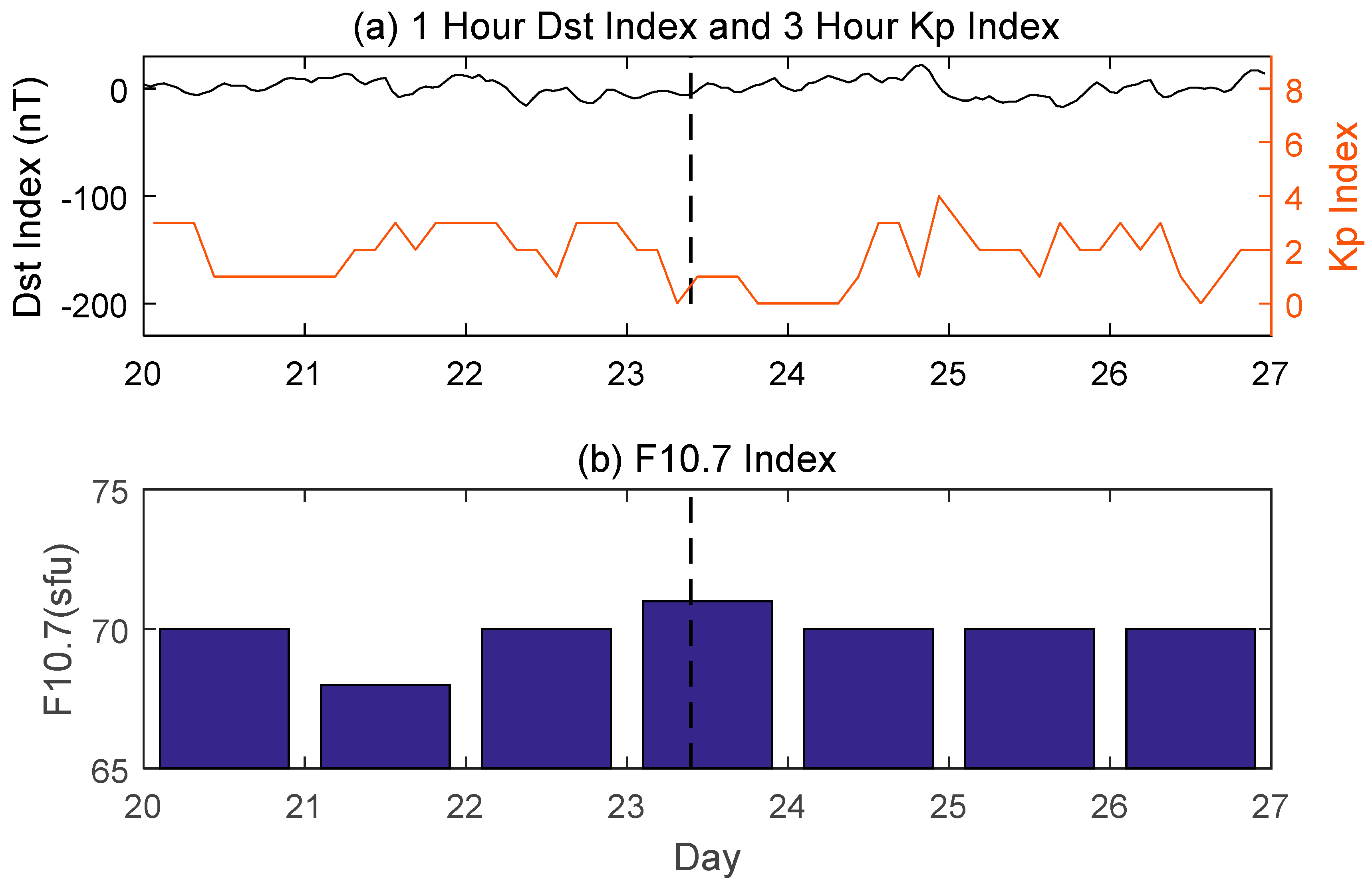
It is well known that solar and geomagnetic activity can affect the ionosphere. Figure 3 shows the geomagnetic index Dst, Kp and solar activity index F10.7 for the week around the Alaska earthquake on 23 January 2018. The data of Dst, Kp are available from http://isgi.unistra.fr/ and the source of solar activity data is http://data.cma.cn/data/. The Dst index indicates the change in the intensity of the horizontal component of geomagnetism. A value higher than −50 indicates a relatively calm period. The Kp index is used to indicate mid-high latitude geomagnetic activities. Generally, values less than 4 can indicate that the geomagnetic activity is calm. The 10.7 cm solar irradiance reflects the solar activities on a corresponding day and the TEC response to the solar activities is instantaneous [29]. It can be seen from Figure 3 that the geomagnetic activity and solar activity on the day of the earthquake are calm. In addition, the data on 23 January of the non-seismic area is used for comparison. Because the geomagnetic and solar activities are calm around the earthquake days, we can conclude that the ionospheric TEC disturbance in the Alaska region was not caused by geomagnetism and solar activity.

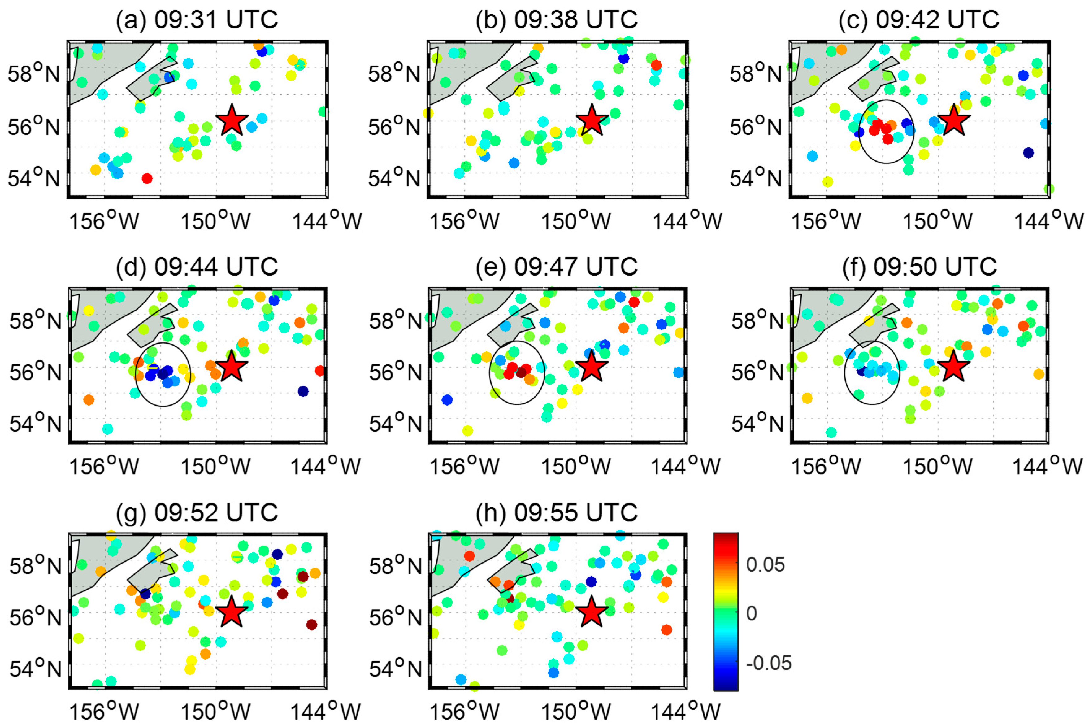
In the study, GPS observations were used to analyze the ionospheric response to the Alaska earthquake on 23 January 2018. Since the TEC is an integral parameter, the observed ionospheric disturbance accounts for a large range of altitudes [24]. However, it is generally assumed that the main contribution to TEC variations appears around the height of the maximum of the ionosphere ionization (F2 layer), with a value of 280 km in this paper. The TEC variations using the filter to eliminate the trend of SIPs motion and ionospheric background changes are most probably related to the earthquake [30]. Other common ionospheric anomalies basically will not have a correlation between the time and distances. The occurrence time of this disturbance coincides with the earthquake. From Figure 4, the ionospheric anomalies are detected about 10 min after the main shock. At around 9:43 UTC, the anomalies appeared a few hundred kilometers from the epicenter. The amplitude of the TEC disturbance can reach a magnitude of 0.06 TEC units (TECU, 1 TECU = 10¹⁶ e/m²). The value of filtered TEC observation turned from positive (Figure 4c) to negative (Figure 4d), then turned to positive (Figure 4f) for the same region as shown in the 09:44 UT and 09:47 UT. The results show that the disturbance is an N-shaped wave and its perturbation period is about 5 min. After 09:52 UT, no TEC disturbance can be detected. Both positive and negative disturbances were detected in the southwest of the epicenter. Compared to the southwest, no disturbance was observed in the northeast.

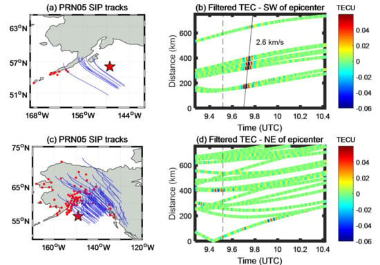
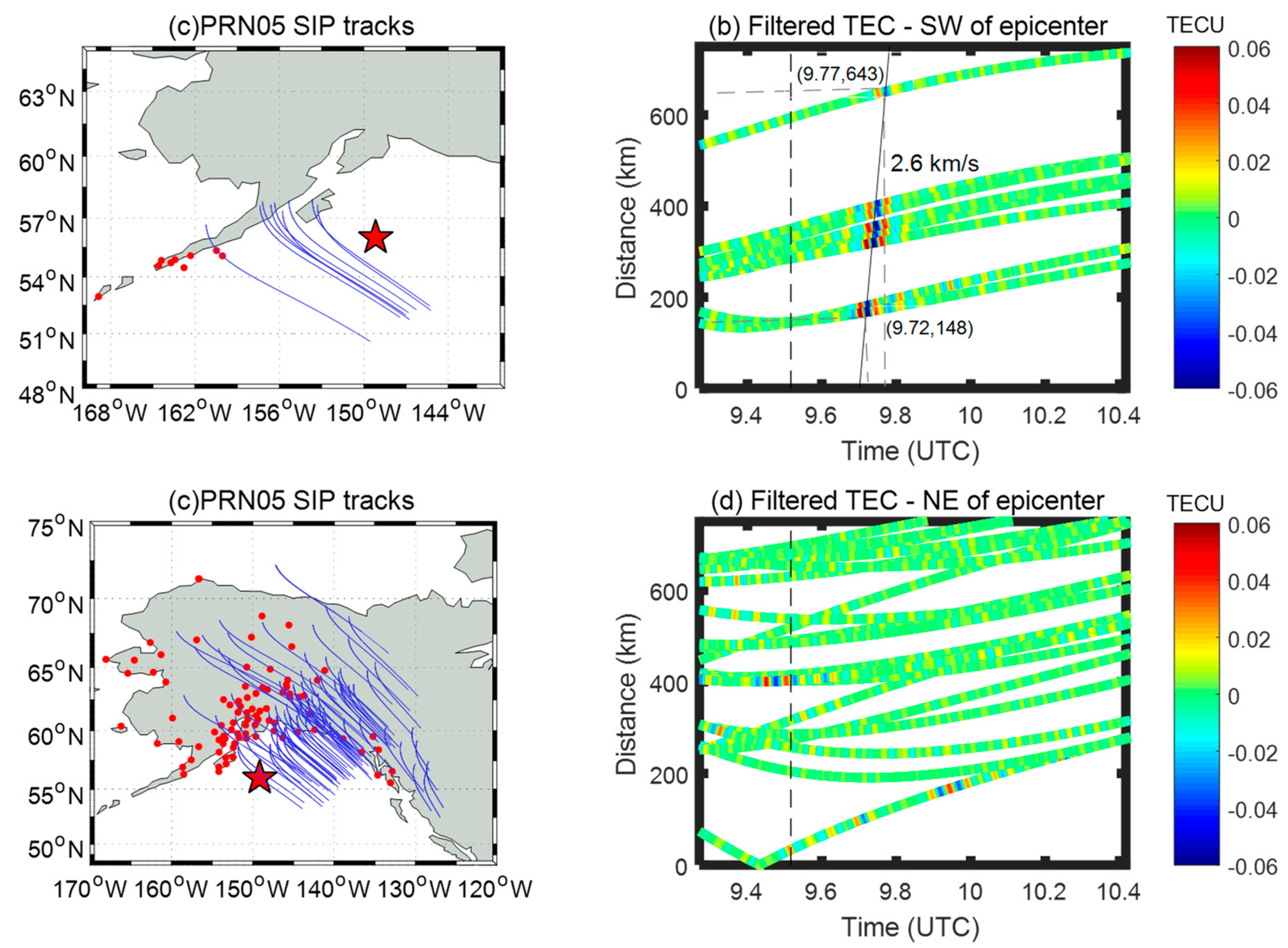
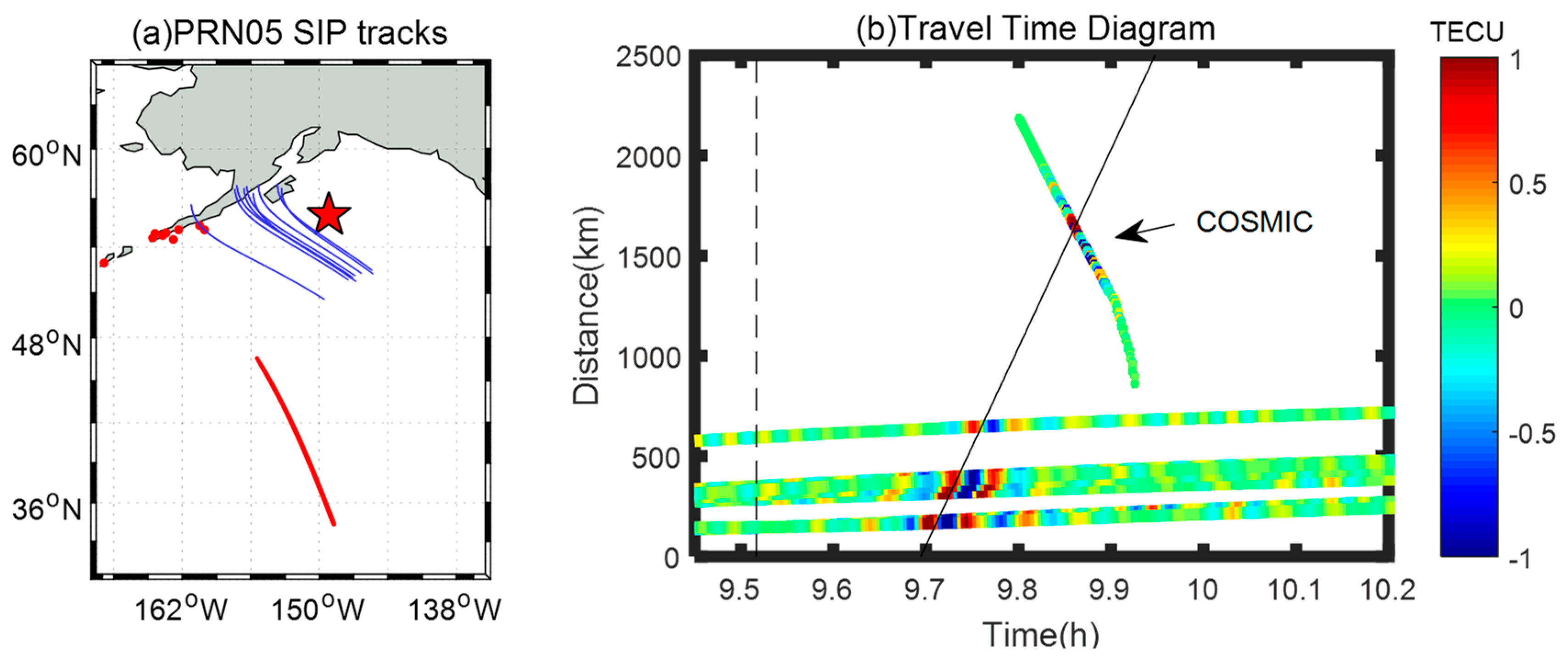
Figure 5 shows an alternate visualization of the ionospheric TEC perturbation after the earthquake. From Figure 5a,c, it can be seen that the SIP tracks relatively covering the epicenter. Figure 5b,d are the travel time diagram of the filtered TEC series, which is obtained by taking the time as the x-axis and y-axis distance between the SIP tracks and the epicenter as the ordinate. The filtered TEC series is divided into two parts by the SIPs in the southwest and northeast of the epicenter. About ten minutes after the earthquake, it can be seen that the observation in the southwest direction of the epicenter can clearly observe the disturbance with an amplitude of about 0.06 TECU. A linear fitting is performed based on the location of the maximum disturbance which has been shown in Figure 5b. The propagation velocity of the TEC disturbance can be estimated by the least square fitting, which is about 2.6 km/s, namely, v = ds/dt = (643 km – 148 km)/((9.773 − 9.721) × 3600) ≈ 2.6 km/s, while the observations in the northeast direction have no obvious disturbance in Figure 5d. This asymmetric disturbance needs to be further studied with more observations in the future, particularly the effect of non-uniform observation geometry [15].

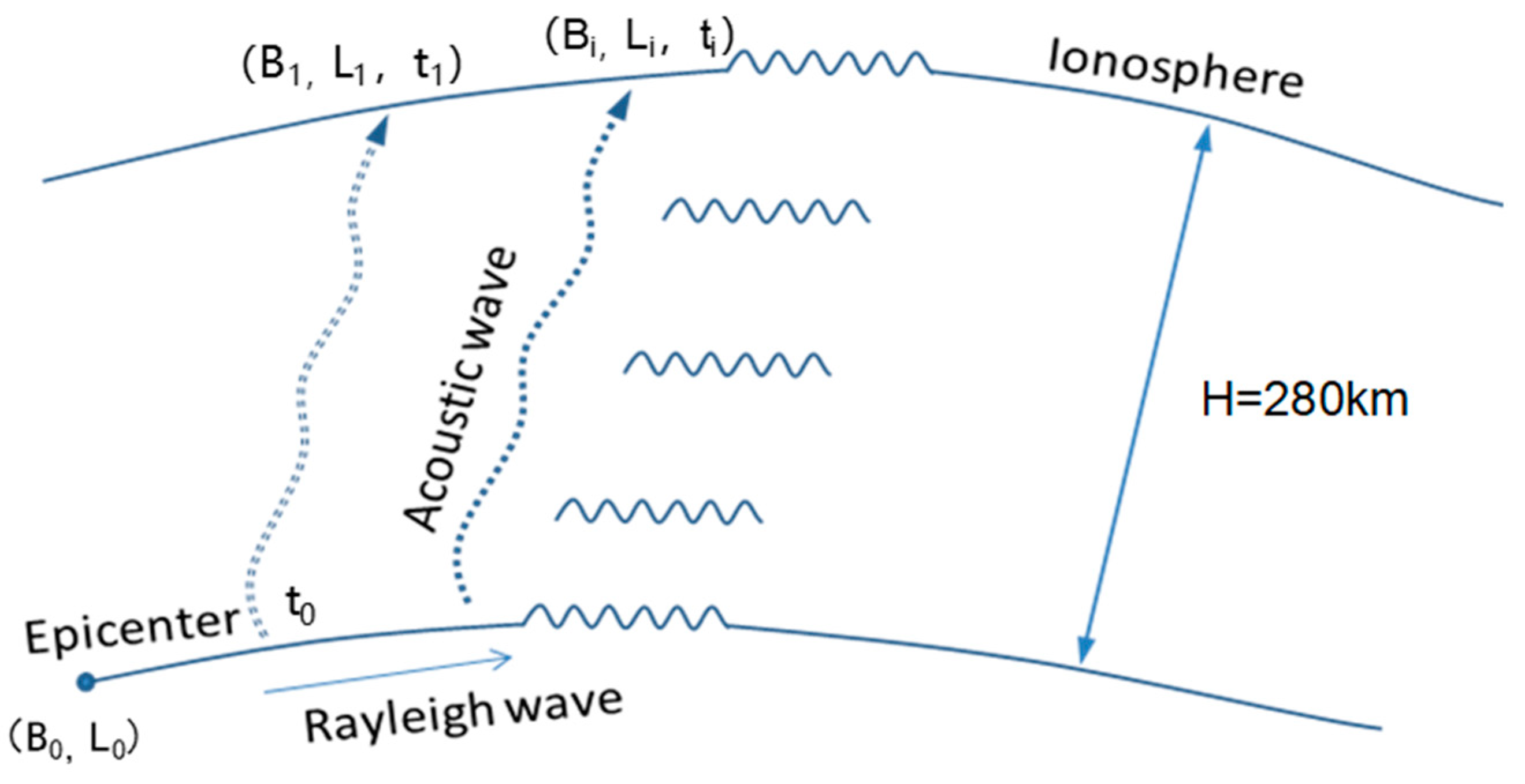
In order to validate the observation results, the epicenter position is estimated from seismic ionospheric disturbances based on the point source propagation around the epicenter with the estimated horizontal velocity in different directions [5]. The acoustic waves generated by the earthquake rupture propagate in all directions around the epicenter. It can be approximated that the trajectory of acoustic waves propagating from the ground to the ionosphere is a straight line [8]. It takes time for the excited acoustic wave propagating from the surface to the ionosphere, as shown in Figure 6. This wave propagates substantially in the vertical direction [22]. The acoustic wave propagation formula can be converted by the following equation:

$$R\arccos \left(\sin B_0\sin B_i+\cos B_0\cos B_i\cos \left(L_0-L_i\right)\right)=v_R·\left(t_i-t_0\right)$$

(3)

where R is the Earth radius, $B_0$ and $L_0$ are the latitude and longitude of the location of epicenter we want to be obtained, $B_i$ and $L_i$ are the latitude and longitude of the location where the disturbances were detected, $t_0$ is the time of acoustic waves propagating from the surface to the ionosphere, $t_i$ is the time difference of the earthquake and disturbance, $v_R$ is the speed of the CIDs.

We brought the disturbance information obtained in Figure 4 and Figure 5 into Equation (3) and calculated $B_0$ and $L_0$ by the measurement adjustment method. The latitude and longitude of the estimated epicenter location is 55.705° N and 148.773° W. This result is slightly different from the actual epicenter position (56.004° N, 149.166° W). The difference between the actual epicenter and the estimated epicenter is considered reasonable. On the one hand, the source of the disturbance is not strictly located at the center of the earthquake rupture [31]. On the other hand, the disturbance can shift by several kilometers from its surface location due to vertical variations of the wave speed as well as horizontal winds [8]. Therefore, combined with the correlation between the disturbance and the location of the epicenter, it can be considered that this CID is caused by the Alaska earthquake.

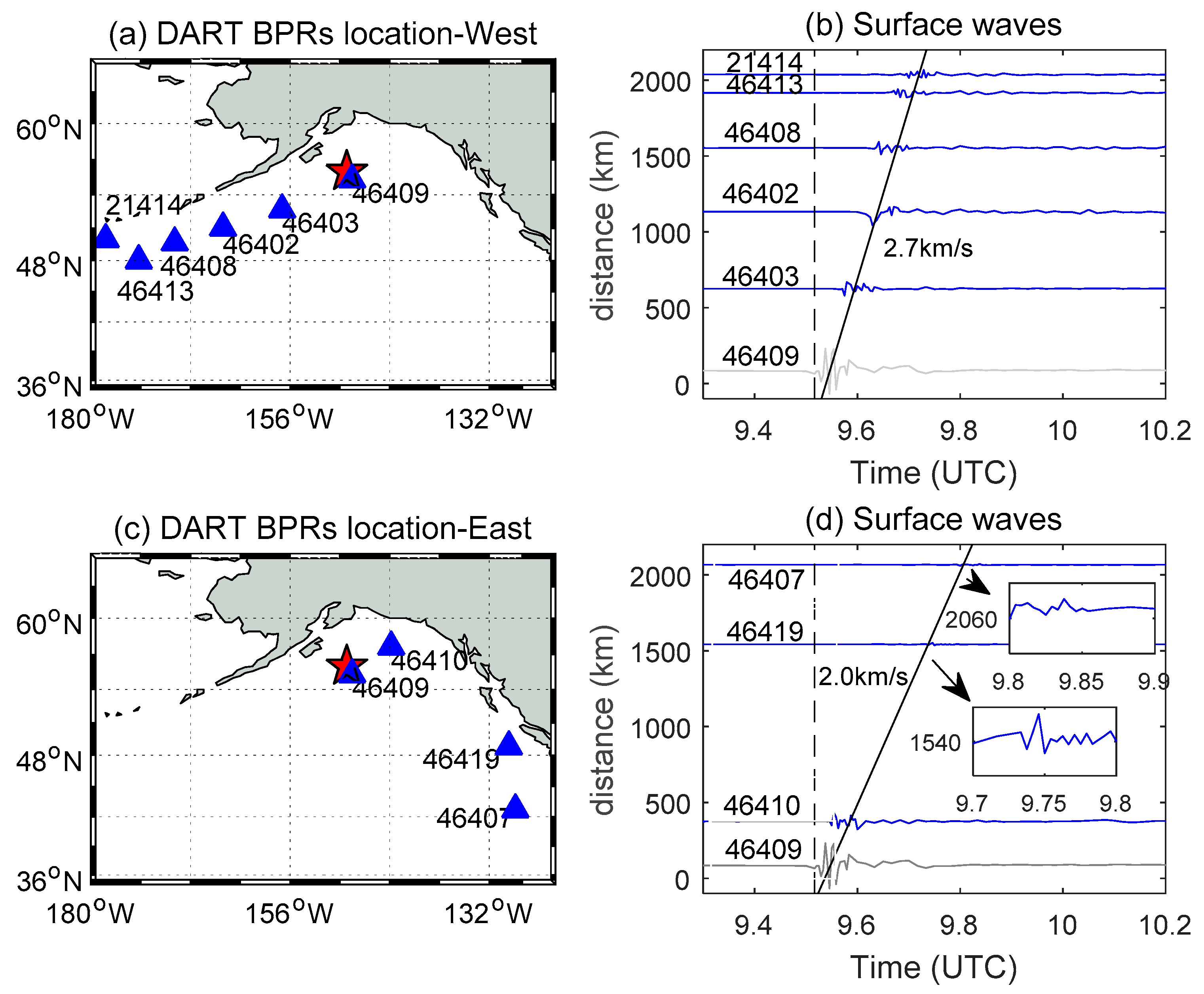
The bottom pressure values from DART BPRs are corrected for temperature effects and the pressure is converted to an estimated height of the ocean surface above the seafloor by using a constant 670 mm/psia. BPR can record not only the pressure changes caused by sea surface fluctuations but also the vertical movement of the seabed. It is a fact that the deep ocean is an ideal low-pass filter, which allows for Rayleigh waves, tsunamis, and other long-period events to be detected by simply measuring the pressure at a fixed point on the seafloor [32]. 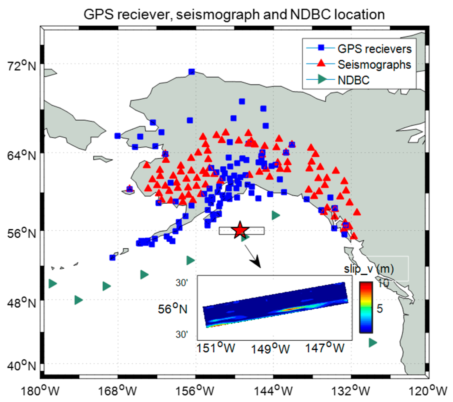Figure 7 is the detrended sea level change in the vicinity of the epicenter recorded by DART BPRs. The linear trend and constant terms are removed by least squares, leaving only the height change of the sea level. A total of 9 DART BPRs observations within 2000 km were used. The location of the sites is shown in Figure 1. The BPR series released by DART usually have a tidal report interval of 15 min at rest. When the submarine pressure disturbance is detected, the sampling rate can reach 1 min or 15 s [32]. The sampling rate of the DART BPR data used in the study is 1 min. Station 46409 is too close to the epicenter, and its seismic impact cannot be regarded as the point source. Therefore, the data of station 46409 was eliminated when fitting. From Figure 7b, a disturbance at the speed of about 2.7 km/s on the seafloor can be clearly observed on the west of the epicenter, which is consistent with the CIDs propagation velocity detected by the GPS data. There is a significant disturbance within 700 km. As the distance increases, the fluctuation of the vertical data on the ground is significantly reduced. A comparison with the disturbance can indicate that the CID is caused by the wave on the seafloor. On the east of the epicenter, a disturbance at a speed of about 2.0 km/m was observed. Station 46419 and 46407 have disturbances with small amplitudes and the enlarged views, presented in the sub-graphs in Figure 7d.

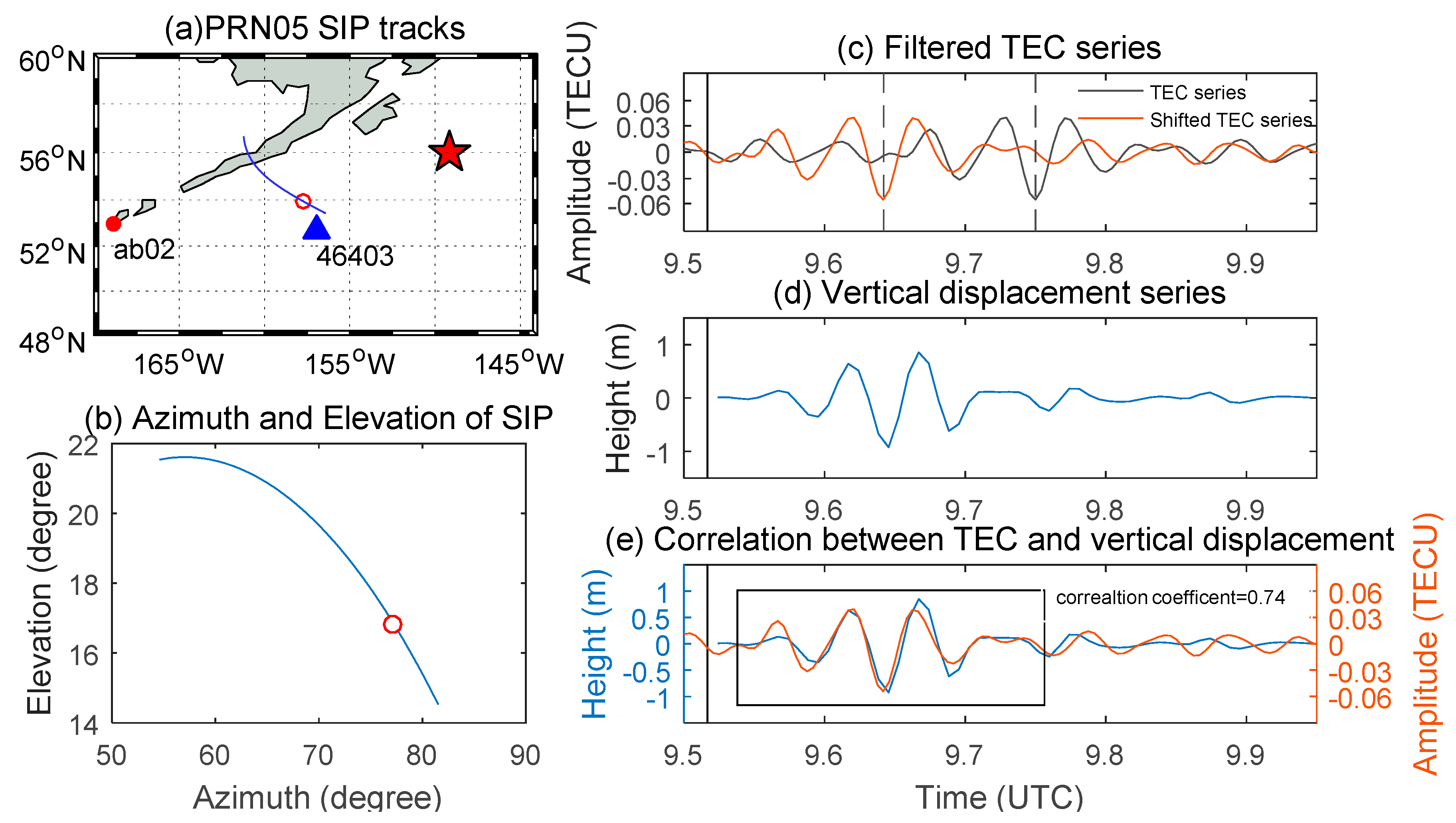
Figure 8 shows the correlation between filtered TEC and DART buoy data. The DART station 46403, which is just located below the satellite puncture point as shown in Figure 8a, is used for the analyses. The black observation in Figure 8c is the filtered TEC series from station AB02 and the orange line is the copy of the black one shifted 6.7 m in advance. The correlation coefficient between the shifted TEC disturbance series and the vertical ground displacement is 0.74. This shows that the vertical displacement of the ground is very similar to the waveform of the TEC disturbance series. It is expected that the distortion of observed waveforms could be induced by the satellite movement. Fortunately, the radial movement is small when compared to the CID scale in 10 min. For the quasi-radial propagation disturbance, the satellite motion effect was ignored [18]. The ionospheric disturbance is the same as the waves obtained from BPRs, but it takes a certain time for the excited acoustic wave to propagate from the surface to the ionosphere.

The coseismic horizontal acoustic wave above the focal region is a possible source of the coseismic ionospheric disturbance. It is induced by the refraction of the upward atmospheric pulse due to the vertical neutral density gradient. However, the sound speed at the ionospheric height is around 1 km/s. Therefore, the detected CIDs are mostly related to the Rayleigh wave that propagates with a much higher speed (~3.0–4.5 km/s) [8,21]. Note that the locations of CID and DART BPRs are shown in Figure 5 and Figure 7, and the 2.6 km/s propagating CID is just above the region where the wave group velocity is about 2.7 km/s. However, other superpositions of acoustic and Rayleigh waves may affect CIDs and make the apparent velocity between the acoustic and Rayleigh waves [18,24], which needs to be further investigated with the available data in the future.

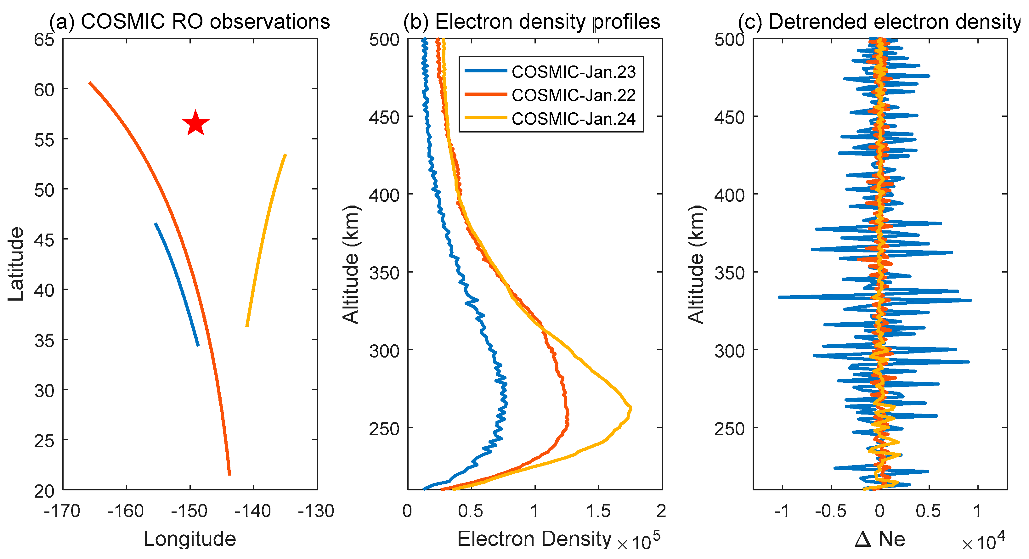
The observations from GPS radio occultation measurements were also used to compare them with the ground-based GPS-VTEC observations. In Figure 9, the radio occultation measurements from Formosat-3/COSMIC are shown. Most of the occultation events last from 300 to 600 s. The ground projection (the blue trajectory) of the occultation points in the COSMIC radio occultation event which starts at 9:48 UTC, is shown in Figure 9a. The ground projections of the radio occultation points at 08:51 UTC the day before (the red curve) and at 10:25 UTC the day after (the yellow curve) measured at the same position are shown for comparison. In Figure 9b, ionospheric plasma density perturbations above the earthquake can be observed in the electron density profile of the region from 200 to 500 km. Compared with the observations of the day before and the day after, the electron density after the earthquake is significantly smaller. In the case of ruling out the influence of solar and geomagnetic activities, the phenomenon of a significant decrease in electron density is considered to be caused by the earthquake. A moving average filter was used to extract trend items during data processing [21]. The observation accuracy of the cosmic electron density data is on the order of 10 cubic degrees. From Figure 9c, it can be clearly seen that the detrended data on the 23rd January is much larger than the data on the 22nd and 24th January, and its magnitude also indicates that this is not caused by the observation error. It can be observed that at the height where the electron density (250 km–350 km) is larger, the amplitude of this COSMIC disturbance is more obvious.

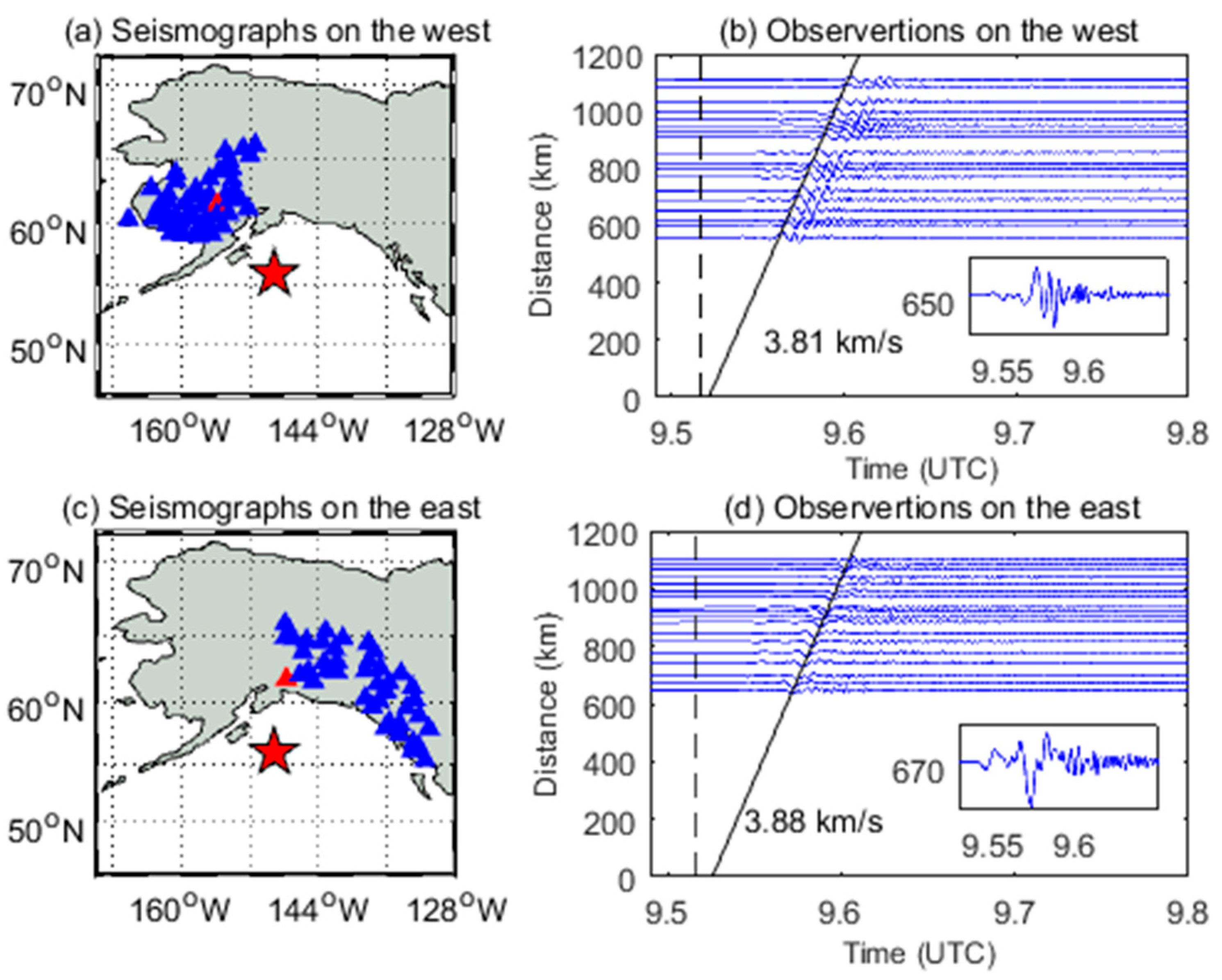
COSMIC radio occultation data with observations from ground-based GPS stations were combined from Figure 10. Since the TEC and electron density are not a single linear relationship, the perturbed waveforms cannot be compared. Thus, the waveform data shown in Figure 10 are normalized by the maximum amplitude. The time of the perturbation coincides with the propagation distance which is very similar to the TEC observations. These results indicate that the wave has reached about 300 km altitude and indeed causes changes in the vertical structure of the ionosphere. The results of Figure 10 support the conclusion that the perturbation of electron density is not an error but is probably caused by the earthquake. The vertical ground motions from the observations of 91 broadband seismographers are presented in Figure 11. The vertical component in the east and west directions are shown in Figure 11b,d, respectively. It can be observed that the Rayleigh waves propagated in all directions. Based on the arrival times of the Rayleigh waves at stations with different distances, the group velocity of the surface Rayleigh wave is estimated to be approximately 3.8 km/s in the west and 3.9 km/s in the east directions. It should be pointed out that the Rayleigh wave appearance epoch is almost at the onset of the earthquake according to the linear fitting estimation. Not only the Rayleigh wave propagation speed at the surface is different, but the vertical ground motions are also observed to be different. This observation is related to the fact that the Alaska earthquake occurred as the result of strike-slip faulting within the shallow lithosphere of the Pacific plate [24]. Focal mechanism solutions indicate that faulting occurred on a steeply dipping fault striking either west-southwest or north-northwest. The first apparent motion observed on the west side is positive while the first one on the east side is negative. Since not enough GPS observations are available to see the ionospheric disturbances over the Alaska region, it is unlikely to make a comparative analysis at present. The Rayleigh wave-induced CID at such a speed is possible [23]. It is believed that the anisotropy of the Rayleigh wave could be an important source of CID propagation divergence in different directions [18].

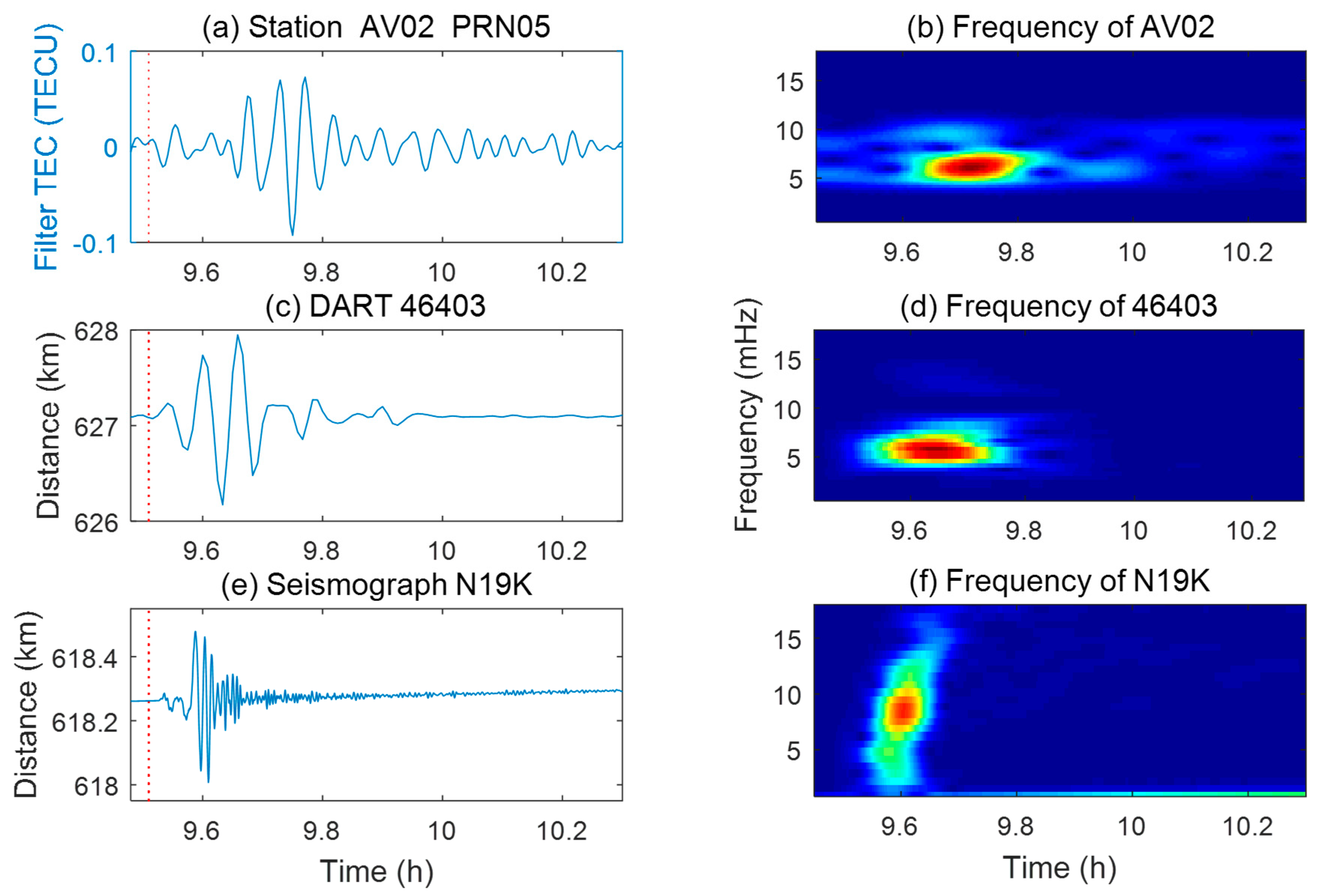
The TEC perturbation time series obtained from GPS dual-frequency observations can be used to analyze the amplitude, duration and propagation velocity of the disturbance. However, the time domain analysis can only reflect the change of the amplitude of the signal, so the frequency domain analysis of the disturbance is performed by using the fast Fourier transform (FFT). In Figure 12, the disturbance series extracted from the observations are shown on the left, and on the right is the spectrum distribution obtained by Fourier transform. The moment when the disturbance occurs can be clearly observed from Figure 12. The power spectrum peak at the corresponding time is also obvious. In Figure 12b, the TEC series of the station AV02 were analyzed and the corresponding frequency of the power extremum was 6.1 mHz. Figure 12d shows the frequency of vertical ground motions from DART BRP which has a corresponding frequency of the power extremum of 5.8 mHz. From Figure 12b,d, the perturbation frequency of the CIDs observed by the GPS satellite is similar to the BPRs data. Combining the conclusions obtained in Figure 8, it can be considered that there is a strong similarity between the two disturbances. The coseismic ionospheric effect is a result of the upward propagation acoustic wave induced by the Rayleigh wave rather than the direct effect of the focal rupture [33]. While Figure 12f shows the frequency of vertical ground motions from seismographers N19K (60.813° N, 154.484° W) with a center of 8.1 mHz. It can be seen from this figure that the power enhances significantly with the arrival of large amplitude surface Rayleigh waves. Combined with the velocity of the dispersion map and the perturbation fit [22], it can be determined that this perturbation is an ionospheric disturbance caused by Rayleigh waves. The frequency of the wave observed by the seismometers is greater than the waves obtained from DART stations and GPS receivers. This also proves that the detected CIDs are mostly related to the Rayleigh wave for another point of view [6].

4. Conclusions

In this paper, the ionospheric response to the 2018 Mw = 7.9 earthquake in Alaska is investigated. The results clearly show a disturbance in the ionosphere around the earthquake about 10 min after the earthquake. The ionospheric disturbances following the 2018 Mw = 7.9 Alaska earthquake are inhomogeneous and directional. From DART data, a disturbance at the speed of about 2.7 km/s on the seafloor can be clearly observed on the west of the epicenter, which is consistent with the coseismic ionospheric disturbances (CIDs) propagation velocity detected by GPS data. From seismograph observations, the velocities and waveforms of the ground vertical motion observed on the east and west sides of the epicenter are different. The first apparent motion observed on the west side is positive while the first one on the east side is negative. According to the spectrum analysis, it can be confirmed that the disturbance is a directional Rayleigh wave when propagating. The directional features appear to be mainly caused by the vertical motions of the seafloor and the ground. We believe that the regional difference of Rayleigh wave velocity should be one of the important reasons for the diversity of the characteristics of the coseismic ionospheric propagation.

References

1. Davies, K.; Baker, D.M. Ionospheric effects observed around the time of the Alaskan earthquake of March 28, 1964. J. Geophys. Res. 1965, 70, 2251–2253. [Google Scholar] [CrossRef]
2. Yuen, P.C.; Weaver, P.F.; Suzuki, R.K.; Furumoto, A.S. Continuous, Traveling Coupling between Seismic Waves and the Ionosphere Evident in May 1967 Japan Earthquake Data. J. Geophys. Res. 1969, 74, 2256–2264. [Google Scholar] [CrossRef]
3. Occhipinti, G.; Dorey, P.; Farges, T.; Lognonné, P. Nostradamus: The radar that wanted to be a seismometer. Geophys. Res. Lett. 2010, 37, 1480–1493. [Google Scholar] [CrossRef]
4. Calais, E.; Minster, J.B. GPS detection of ionospheric perturbations following the January 17, 1994, Northridge Earthquake. Geophys. Res. Lett. 1995, 22, 1045–1048. [Google Scholar] [CrossRef]
5. Astafyeva, E.; Heki, K.; Kiryushkin, V.; Afraimovich, E.; Shalimov, S. Two-mode long-distance propagation of coseismic ionosphere disturbances. J. Geophys. Res. Space Phys. 2009, 114. [Google Scholar] [CrossRef]
6. Jin, S.; Jin, R.; Li, J.H. Pattern and evolution of seismo-ionospheric disturbances following the 2011 Tohoku earthquakes from GPS observations. J. Geophys. Res. Space Phys. 2015, 119, 7914–7927. [Google Scholar] [CrossRef]
7. Rolland, L.M.; Lognonné, P.; Astafyeva, E.; Kherani, E.A.; Kobayashi, N.; Mann, M.; Munekane, H. The resonant response of the ionosphere imaged after the 2011 off the Pacific coast of Tohoku Earthquake. Earth Planets Space 2011, 63, 62. [Google Scholar] [CrossRef]
8. Artru, J.; Farges, T.; Lognonn, P. Acoustic waves generated from seismic surface waves: Propagation properties determined from Doppler sounding observations and normal-mode modelling. Geophys. J. Int. 2004, 158, 1067–1077. [Google Scholar] [CrossRef]
9. Ducic, V.; Artru, J.; Lognonné, P. Ionospheric remote sensing of the Denali Earthquake Rayleigh surface waves. Geophys. Res. Lett. 2003, 30. [Google Scholar] [CrossRef]
10. Calais, E.; Minster, J.B. GPS, earthquakes, the ionosphere, and the Space Shuttle. Phys. Earth Planet. Inter. 1998, 105, 167–181. [Google Scholar] [CrossRef]
11. Cahyadi, M.N.; Heki, K. Coseismic ionospheric disturbance of the large strike-slip earthquakes in North Sumatra in 2012: Mw dependence of the disturbance amplitudes. Geophys. J. Int. 2015, 200, 116–129. [Google Scholar] [CrossRef]
12. Heki, K.; Ping, J. Directivity and apparent velocity of the coseismic ionospheric disturbances observed with a dense GPS array. Earth Planet. Sci. Lett. 2005, 236, 845–855. [Google Scholar] [CrossRef] [Green Version]
13. Liu, J.Y.; Tsai, H.F.; Lin, C.H.; Kamogawa, M.; Chen, Y.I.; Lin, C.H.; Huang, B.S.; Yu, S.B.; Yeh, Y.H. Co-seismic ionospheric disturbances triggered by the Chi-Chi earthquake. J. Geophys. Res. Space Phys. 2010, 115. [Google Scholar] [CrossRef]
14. Afraimovich, E.L.; Ding, F.; Kiryushkin, V.V.; Astafyeva, E.I.; Jin, S.; Sankov, V.A. TEC response to the 2008 Wenchuan Earthquake in comparison with other strong earthquakes. Int. J. Remote Sens. 2010, 31, 3601–3613. [Google Scholar] [CrossRef] [Green Version]
15. Occhipinti, G.; Rolland, L.; Lognonné, P.; Watada, S. From Sumatra 2004 to Tohoku-Oki 2011: The systematic GPS detection of the ionospheric signature induced by tsunamigenic earthquakes. J. Geophys. Res. Space Phys. 2013, 118, 3626–3636. [Google Scholar] [CrossRef] [Green Version]
16. Astafyeva, E.; Shalimov, S.; Olshanskaya, E.; Lognonné, P. Ionospheric response to earthquakes of different magnitudes: Larger quakes perturb the ionosphere stronger and longer. Geophys. Res. Lett. 2013, 40, 1675–1681. [Google Scholar] [CrossRef] [Green Version]
17. Shinagawa, H.; Tsugawa, T.; Matsumura, M.; Iyemori, T.; Saito, A.; Maruyama, T.; Jin, H.; Nishioka, M.; Otsuka, Y. Two-dimensional simulation of ionospheric variations in the vicinity of the epicenter of the Tohoku-oki earthquake on 11 March 2011. Geophys. Res. Lett. 2013, 40, 5009–5013. [Google Scholar] [CrossRef]
18. Jin, S.; Jin, R.; Li, D. GPS detection of ionospheric Rayleigh wave and its source following the 2012 Haida Gwaii earthquake. J. Geophys. Res. 2017, 122, 1360–1372. [Google Scholar] [CrossRef]
19. Jin, S.G. Two-mode ionospheric disturbances following the 2005 Northern California offshore earthquake from GPS measurements. J. Geophys. Res. Space Phys. 2018, 123, 8587–8598. [Google Scholar] [CrossRef]
20. Lay, T.; Ye, L.; Kanamori, H.; Yamazaki, Y.; Cheung, K.F.; Kwong, K.; Koper, K.D. The October 28, 2012 Mw 7.8 Haida Gwaii underthrusting earthquake and tsunami: Slip partitioning along the Queen Charlotte Fault transpressional plate boundary. Earth Planet. Sci. Lett. 2013, 375, 57–70. [Google Scholar] [CrossRef] [Green Version]
21. Ram, S.T.; Sunil, P.S.; Kumar, M.R.; Su, S.Y.; Tsai, L.C.; Liu, C.H. Coseismic Travelling Ionospheric Disturbances (CTIDs) during the Mw 7.8 Gorkha, Nepal Earthquake on 25 April 2015 from ground and space borne observations. J. Geophys. Res. 2017, 122, 10669–10685. [Google Scholar]
22. Rolland, L.M.; Lognonné, P.; Munekane, H. Detection and modeling of Rayleigh wave induced patterns in the ionosphere. J. Geophys. Res. Space Phys. 2011, 116. [Google Scholar] [CrossRef]
23. Maruyama, T.; Tsugawa, T.; Kato, H.; Ishii, M.; Nishioka, M. Rayleigh wave signature in ionograms induced by strong earthquakes. J. Geophys. Res. 2012, 117. [Google Scholar] [CrossRef]
24. Astafyeva, E.; Rolland, L.M.; Sladen, A. Strike-slip earthquakes can also be detected in the ionosphere. Earth Planet. Sci. Lett. 2014, 405, 180–193. [Google Scholar] [CrossRef]
25. Lay, T.; Ye, L.; Bai, Y.; Cheung, K.F.; Kanamori, H. The 2018 MW 7.9 Gulf of Alaska earthquake: Multiple fault rupture in the Pacific plate. Geophys. Res. Lett. 2018, 45, 9542–9551. [Google Scholar] [CrossRef]
26. Cai, C.; Liu, Z.; Xia, P.; Dai, W. Cycle slip detection and repair for undifferenced GPS observations under high ionospheric activity. GPS Solut. 2013, 17, 247–260. [Google Scholar] [CrossRef]
27. Perevalova, N.P.; Sankov, V.A.; Astafyeva, E.I.; Zhupityaeva, А.S. Threshold Magnitude for Ionospheric Response to Earthquakes. J. Atmos. Sol.-Terr. Phys. 2013, 108, 77–90. [Google Scholar] [CrossRef]
28. Dautermann, T.; Calais, E.; Mattioli, G. GPS Detection and Energy Estimation of the Ionospheric Wave caused by the July 13th, 2003 Explosion of the Soufriere Hills Volcano, Montserrat. J. Geophys. Res. 2008, 114. [Google Scholar] [CrossRef]
29. Mansoori, A.A.; Khan, P.A.; Bhawre, P.; Gwal, A.K.; Purohit, P.K. Variability of TEC at mid latitude with solar activity during the solar cycle 23 and 24. In Proceedings of the 2013 IEEE International Conference on Space Science and Communication (IconSpace), Melaka, Malaysia, 1–3 July 2013. [Google Scholar]
30. Tsugawa, T.; Saito, A.; Otsuka, Y.; Nishioka, M.; Maruyama, T.; Kato, H.; Nagatsuma, T.; Murata, K.T. Ionospheric disturbances detected by GPS total electron content observation after the 2011 Tohoku earthquake. Earth Planets Space 2011, 63, 875–879. [Google Scholar] [CrossRef]
31. Okabe, M. Analytical expressions for gravity anomalies due to homogeneous polyhedral bodies and translations into magnetic anomalies. Geophysics 1979, 44, 730–741. [Google Scholar] [CrossRef]
32. US Department of Commerce; National Oceanic and Atmospheric Administration; National Weather Service; National Data Buoy Center. Deep-Ocean Assessment and Reporting of Tsunamis; National Geophysical Data Center, NOAA: Silver Spring, MD, USA, 2005. [CrossRef]
33. Jin, S.; Occhipinti, G.; Jin, R. GNSS ionospheric seismology: Recent observation evidences and characteristics. Earth-Sci. Rev. 2015, 147, 54–64. [Google Scholar] [CrossRef]
Figure 1. The distribution of GPS stations, seismographs and NDBC (National Data Buoy Center) stations around the epicenter. The red pentagram represents the epicenter. The square points represent GPS stations, the red triangles represent seismographs stations and green triangles represent NDBC stations. The sub-picture shows the finite fault of the earthquake (https://earthquake.usgs.gov/earthquakes). Strike-slip-faulting events of the size of the earthquake are typically about 230 × 30 km.
Remotesensing 11 00901 g001
Figure 2. The filtered TEC (total electron content) observed by station AV26 and PRN 05 during the Alaska earthquake on 23 January 2018. In (a), the blue line is the SIPs (sub-ionospheric points) track. The star and the point show the location of the epicenter and AV26 station. (b) shows the elevation angle of the satellite (the blue line) and the distance between the SIPs and the epicenter (the red line). (c) is the TEC obtained through different cutoff frequencies.
Remotesensing 11 00901 g002
Figure 3. The geomagnetic index Dst, Kp and solar activity index F10.7 for the week around the Alaska earthquake on 23 January 2018. The dotted lines indicate the time of the earthquake.
Remotesensing 11 00901 g003
Figure 4. The filtered TEC variations from the 9:31 to 9:55 UTC following the Alaska earthquake. The red star indicates the location of the epicenter of the Alaska earthquake and the dots represent the position of the sub-ionospheric points (SIPs). The color of the dots indicates the amplitude of the filtered TEC disturbances.
Remotesensing 11 00901 g004
Figure 5. The ionospheric responses to the Alaska earthquake. The left is the SIP tracks between the PRN05 and the stations, and the right is the travel time diagram of filtered TEC series. The dashed line indicates the time of the earthquake eruption, and the diagonal line is used to fit the speed of the TEC disturbances. Different colors show the magnitude of TEC interference.
Remotesensing 11 00901 g005
Figure 6. The diagram of disturbances propagation.
Remotesensing 11 00901 g006
Figure 7. The sea level change in the vicinity of the epicenter recorded by Bottom Pressure Records (BPRs). The location of the site is shown in (a,c). The sub-graphs in the (d) are the enlarged views of station 46419 and 46407.
Remotesensing 11 00901 g007
Figure 8. The correlation between filtered TEC and DART (Deep-ocean Assessment and Reporting of Tsunamis) buoy data. (a) shows the location of DART station 46403 and the satellite puncture. (b) shows the observational geometry between the station AV02 and the GPS satellite. The hollow circles in (a,b) show the moment when the earthquake struck. (c) shows the filtered TEC series of station AV02 in black and the copy of the filtered TEC series shifted 6.7 min advance in orange. (d) shows the vertical displacement series of station 46403. (e) shows the correlation between the filtered TEC series shifted 6.7 min forward and vertical displacement series.
Remotesensing 11 00901 g008
Figure 9. The ionospheric electron density from COSMIC (Constellation Observing System for Meteorology, Ionosphere and Climate) radio occultation data. (a) shows the ground projections of COSMIC radio occultation observations. (b) shows the electron density profiles observed with COSMIC satellites. (c) is the detrended COSMIC electron density perturbations. The blue trajectory represents the observations of the Alaska earthquake, and the red and yellow curves represent the result from observations of COSMIC the day before the earthquake and the day after the earthquake.
Remotesensing 11 00901 g009
Figure 10. The results of the combination of COSMIC radio occultation and observations of ground-based GPS stations. (a) shows the puncture point trajectory of several GPS stations and the ground projection of radio occultation observations. (b) combines the normalized filtered TEC series with the detrended COSMIC electron density perturbation and the diagonal line is used to fit the speed of the TEC disturbances.
Remotesensing 11 00901 g010
Figure 11. The vertical ground motions from the observations of 91 broadband seismographers. The location of the stations in the east and west directions of epicenter are shown in (a,c). The vertical components in the east and west directions are shown in (b,d). The sub-graphs in the (b,d) show the enlarged views of two stations at 650 km and 670 km from epicenter respectively and the location of two stations are shown in the (a,c) with red triangles.
Remotesensing 11 00901 g011
Figure 12. The disturbance series extracted from the observations and the spectrum distribution obtained by Fourier transform. (a,c,e) show the data from the GPS, DART and seismograph respectively. (b,d,f) show the spectrum distribution of corresponding observations.
Remotesensing 11 00901 g012