1. Introduction
Hyperspectral imagery (HSI) has a vast range of applications, such as in mineral exploration [
1], anomaly detection [
2], and supervised classification [
3,
4,
5]. Among these applications, the classification of different land covers has attracted lots of attention in the remote sensing community due to the existence of rich spectral and spatial information in HSI. However, classification methods and algorithms need to be improved to be able to handle the large number of spectral bands and spatial information in HSI.
Traditional methods of classification, such as maximum likelihood (ML) [
6], support vector machines (SVMs) [
3], and random forest (RF) [
7], have been and are being widely applied for HSI classification tasks. However, the major drawback of these methods is the fact that they classify data in a spectral domain, that is, they ignore spatial information during the classification process. To address this drawback, the SVM together with composite kernels (SVM-CK) was proposed by Camps-Valls et al. and Fauvel et al. [
8,
9] in order to enhance traditional SVM by considering the spatial information. Although SVM-CK uses features like the mean or the standard deviation to consider the spatial information, these features cannot represent the full content and semantic features of this kind of information. In parallel to this concept, morphological profiles (MPs) [
10], extended MPs (EMPs) [
11], and Markov random fields (MRFs) [
12] were proposed to extract the spatial information. In Reference [
13], advanced versions of these methods were applied on a number of HSI datasets. Although these methods significantly improved the classification performance, their spatial features were manually extracted, which means that prior knowledge and experts’ experiences are of essence [
14,
15,
16].
Recently, deep learning (DL) methods, in which both spectral and spatial information are automatically extracted, have been employed for HSI classification tasks [
17,
18,
19,
20]. Chen et al. [
21] proposed a spectral-spatial classification auto-encoder model in which first, an HSI data cube is preprocessed using principal component analysis (PCA). After that, target pixels along with their neighbors, called PCA-cubes, are extracted from the principal components. Finally, PCA-cubes are unfolded to a 1-D vector form and entered into several stack auto-encoder layers. This scheme, that is, using the local regions to train a 1-D structural method, is also used in Reference [
22]. In another study, Li et al. [
23] developed a novel version of the scheme based on a 1-D convolutional neural network (CNN) and the pixel-pair strategy, to consider both the spectral and spatial information of neighboring pixels.
A major limitation of these methods is that they do not jointly employ both spectral and spatial information for classification. Instead of using a 1-D structure, Zhao et al. [
24] used a novel dimensionality reduction method and a 2-D CNN model to extract spectral and spatial features. These features were stacked together and used for HSI classification. The PCA dimensionality reduction along with EMP were applied in Reference [
13] to enhance both the spectral and spatial feature extractions of the 2-D CNN model. Ma et al. [
14] also applied a spectral dimensionality reduction method to an HSI data cube. Afterwards, the reduced data was fed to a deep 2-D CNN model architecture. The model included several 2-D convolution, deconvolution, pooling, and unpooling layers with the residual connections. Nevertheless, due the application of dimensional reduction processes, these methods may discard some spectral information.To preserve the spectral information and to reduce the computational burden, the stacking spectral patches strategy was proposed in Reference [
15]; nonetheless, the shallow CNN model of this method cannot extract spatial information in an efficient manner. The 1-D CNN and 2-D CNN were proposed by Reference [
25] to extract the spectral and spatial information for classification in a separate manner. He et al. [
26] proposed the application of a 2-D CNN framework with a new manual feature extraction method. These methods obtain good results, despite not using the full capacity of DL methods like joint or automatic spectral-spatial feature extraction.
To address the abovementioned issue, the 3-D structural methods are presented on extracted cubes/patches of the HSI where both spectral and spatial information are jointly extracted. In this context, Chen et al. [
17] applied a 3-D CNN model to jointly extract the spectral and spatial features from the data. Their model contains the 3-D convolution and pooling layers to extract the spectral-spatial features and to decrease their dimensionality, respectively. The 3-D CNN model is also equipped with the residual connections [
27]. Moreover, Liu et al. [
28] applied the transfer learning and virtual sampling strategies to improve the 3-D CNN performance. The feed-forward processing structure let these models reduce the computational burden. As a drawback, these models, as the vector-based methodologies, cannot analyze the full content of spectral-spatial information. Due to limited spatial information in the HSI extracted patches, losing this information leads to a side effect in the classification performance. In general, setting the appropriate spatial size of patches is a controversial issue in these methods [
16,
27,
28,
29].
The recurrent neural network (RNN) as a sequence-based methodology was proposed in Reference [
30]. The intuition behind the use of RNN is to utilize the high computational power of a recurrent analysis for HSI classification. The RNN was combined with CNN by Reference [
31] to boost the model performance. These methods considered the spectral bands of each pixel as a sequence of inputs to recurrently analyze them in the RNN. However, they only considered the spectral information while discarding the spatial one. To address the spatial consideration in the recurrent processing of the spectral information, the Bi-convolutional long short-term memory (CLSTM) was proposed in Reference [
32]. This model applied a bidirectional connection to enhance the process of the spectral feature extraction. The convolutional kernel was also incorporated into the model to consider the neighboring information as well. Nevertheless, the concern of the recurrent processing structure of this model was the spectral feature extraction. That means that the extraction of spatial information is out of the concern of this model. In addition, the training process of this model is extremely time-consuming.
In summary, a joint extraction of the spectral and spatial features in a robust manner with a reasonable computational burden is the main concern in HSI classification. For this purpose, we develop a classification framework with two feature extraction stages. In the first stage, the 3-D CNN is applied to process a high-dimensional HSI cube to effectively extract low-dimensional spectral-spatial features. In the second stage, an innovative structure is designed to consider different pixels of the 3-D-CNN-driven features as a sequence of inputs for the CLSTM. By doing so, deep semantic spectral-spatial features are generated. The main contributions and novelties of the proposed model are briefed as follows.
Unlike previous studies, considering different bands as a sequence for the recurrent analysis, here, for the first time, neighboring pixels are regarded as a sequence to the recurrent procedure.
We build a novel, 3-D HSI classification framework which can jointly extract spectral and spatial features from HSI data. The architecture of this framework enables our model to take full advantage of vector-based and sequence-based learning methodologies in HSI classification.
To deal with the computational burden of CLSTM which makes the training process time-consuming, we take advantage of the 3-D CNN prior to the CLSTM to reduce the huge volume of spectral dimensionality. This strategy efficiently reduces the number of parameters in the recurrent processing of the CLSTM.
The remainder of this paper is organized as follows. The architecture of the proposed classification framework is briefly described in
Section 2.
Section 3 provides the experimental results, analysis, and comparisons. Lastly,
Section 4 draws the concluding remarks of this paper.
2. Methodology
As illustrated in
Figure 1, our DL classification model has three blocks. The first block is applied to extract the shallow low-dimensional spectral-spatial features. The second block is applied to extract the more abstract and semantic spectral-spatial features in a continuous form, and the third one runs the classification task.
For this purpose, let us assume
, where
B is the number of spectral bands and
n is the number of pixels having a ground truth label, namely
. For each member of
X set, the image patches with the size of
(
w is the window size) are extracted, where
is its centered pixel. Accordingly, the
X set can be represented as
. After the extraction of the image patches, each patch,
is fed into Block 1. In this block, the great spectral dimension of the input patch is processed in two convolutional layers, namely CNN1 and CNN2, containing hundreds of 3-D convolutional kernels. The details of these kernels are summarized in
Section 2.1. The function of these layers is to reduce the spectral dimension and to extract shallow spectral-spatial features. After completing the process of Block 1, its output
(
is the number of filters) is fed into the next block.
The outputs of Block 1, are entered into Block 2 with a CLSTM layer in order to make the features more abstract and discriminative. In this layer, the neighboring pixels are regarded as a sequence of inputs (3-D tensors) for the recurrent procedure. To comprehend the 3-D structural processing of this layer, its inputs and states can be presumed as vectors standing on a spatial grid; consequently, the inputs and past states of neighboring pixels can determine the future state in this grid through a recurrent analysis. By doing this, the output of this layer can be represented as
, where
is the number of outputs for Block 2. More detail on this layer is described in
Section 2.2.
Finally, in Block 3, spectral-spatial features, consecutively extracted through pervious blocks, are considered for the membership probability of the classification task. This task is performed in a fully connected layer by a softmax as an activation function.
2.1. Convolutional Layer
According to Reference [
33], a convolutional kernel in a 3-D CNN is applied to simultaneously extract the spectral and spatial features of the input. For the
jth feature map in the
ith layer,
at an
position can be formulated as
where
e,
f, and
g are the width, height, and depth of the 3-D kernel, respectively;
W is the weight of position (
e,
f, and
g) connected to the
k feature map,
b denotes bias, and
stands as an activation function. For the convolutional layers of the proposed model, the biases were omitted and batch normalization (BN) [
34] along with the
norm regularization technique were used. The BN is applied (i) to tackle the internal covariant shift phenomenon and (ii) to make model training possible in the presence of small initial learning rates. Furthermore, a rectified linear unit (ReLU) [
35] is employed as an activation function. After applying these operations, the formulation of the convolutional layer can be rewritten as follows:
where
Note that
is a regularized weight matrix and that
is the output of ReLU activation function.
presents the output of the BN function. Furthermore,
and
respectively display the expectation and variance of each input, and
and
stand as learnable parameters.
In the proposed model, we applied two 3-D CNN layers, CNN1 and CNN2, to process high-dimensional spectral information and the produce shallow spectral-spatial features. After completing the feature extraction process of these two layers, features the spectral dimension of which is 1 are generated. Subsequently, these features are entered to Block 2 where the spatial information is recurrently analyzed in this block.
2.2. Recurrent Layer
In the literature of sequence-based methodology, a long short-term memory [
36] (LSTM) network has been used in a wide range of researches [
36,
37,
38,
39,
40]. The main contribution of the LSTM architecture is to make the network more resistant to either the vanishing or exploding gradient phenomenon, which are the main concerns of an RNN’s training process [
41,
42,
43]. To do so, an LSTM defines a memory cell,
(Equation (4)), which contains the state information at time
t. An input gate
(Equation (5)) and a forget gate
(Equation (6)), respectively, stores and discards a part of the memory cell information. The memory cell,
, is updated by a current memory cell information, named
(Equation (7)). Lastly, the cell,
, is tuned by an output gate,
(Equation (8)). To sum up, these features trap a gradient into a cell to preserve it from vanishing or exploding quickly [
36]. However, as observed in
Figure 2, an LSTM network has one 1-D structure because it applies matrix multiplication (“.” in
Figure 2). Therefore, the LSTM converts the inputs to 1-D vectors prior to any processing. This issue causes the spatial information of the data to be lost.
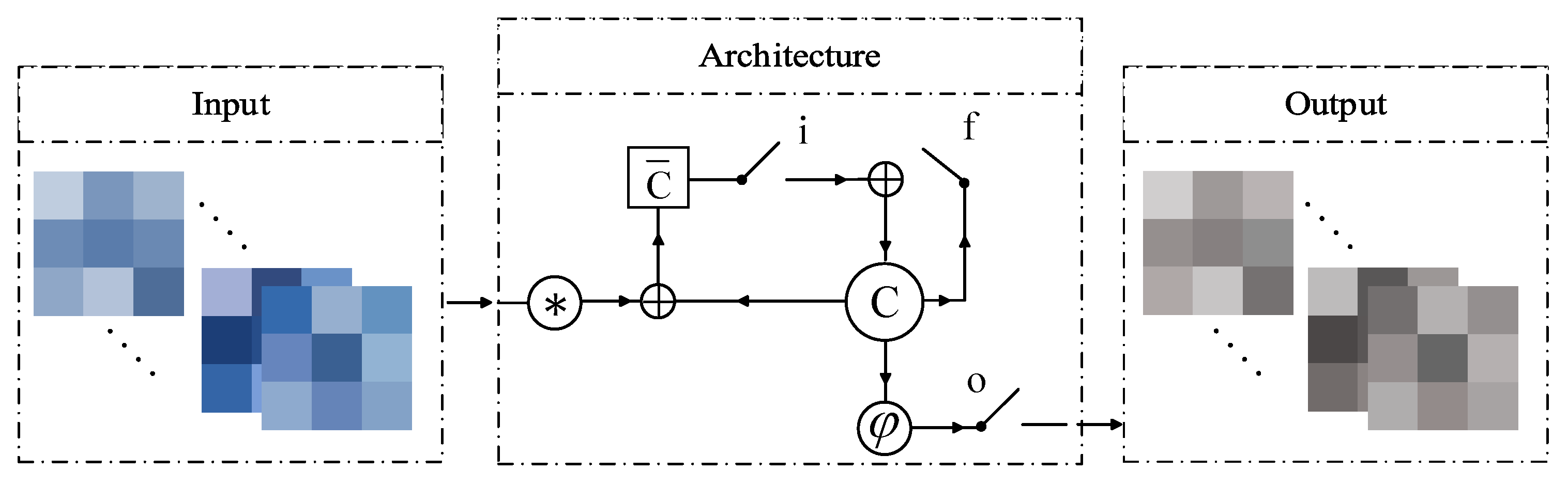
To address this problem, recently, Shi et al. [
44] proposed a CLSTM network using convolutional kernels to perform an LSTM analysis for 3-D structural data. As observed in
Figure 3, by replacing the convolutional operation (“*”) with matrix multiplication, the spatial information is considered in the process of the sequence prediction. Accordingly, the CLSTM is taken into account for Block 2 to analyze the spatial contents of HSI in a recurrent manner while considering the spectral contents. In general, the convolutional operator of the CLSTM is set to consider the spatial information in the recurrent analysis of a temporal observation. However, in this study, the recurrent analysis of CLSTM is directly applied to the spatial dimension. Concurrently, the convolutional operator is incorporated into the model to consider a temporal observation in a recurrent processing of spatial information. According to this strategy, columns of HSI input patches are considered as the sequences of inputs. In the meanwhile, the kernel size of this layer determines how many sequences should be involved in the output generation. Setting the first dimension of the kernel size equal to 1, each sequence generates a one-step prediction. Consequently, by entering the
neighboring pixels’ information to this layer, a
output feature is produced. Therefore, the sequence-based methodology can be applied to capture spatial information for the HSI classification. It should be mentioned that the biases of the original form of the CLSTM network are omitted and that the BN is applied to the output of this layer (Equation (9)). The equations of this layer are arranged as follows:
where
and
are the activation functions,
H is the hidden state, ∘ is the point-wise product, ∗ is convolutional operator, and
W is the weight matrix; e.g.,
is the input-memory cell weight matrix.
We establish this architecture to recurrently analyze the spatial content of input cubes according to the assumption that neighboring pixels might belong to the same material/category. Note that it is quite possible that some cubes are extracted from the boundary of two or more categories. Accordingly, there are two different scenarios in an HSI classification using the CLSTM, both of which are discussed in the following.
In the first scenario, which has a homogeneous area assumption, pixels in a data cube belong to the same material. Since each pixel is entered into the model along with its neighboring pixels, extracted data cubes/patches are expected to have overlaps. These overlaps (i.e., common pixels among patches) have been considered by CLSTM. Since the proposed model has the capability to consider correlations among joint pixels in different patches, we call it patch-related convolutional long short-term memory (PRCLSTM).
In the second scenario, which is based on a heterogeneous area assumption, the patches processed in the model contain different materials. In this case, the inner structure of the CLSTM, which is controlled by gate units, can switch off irrelevant input connections and expose the relevant part of the memory information in the state-to-state transition. From the perspective of these two scenarios, it can be concluded that CLSTM guarantees an excellent performance in the both homogeneous and heterogeneous areas commonly available in HSI datasets.
3. Experimental Results
3.1. Experiment Data
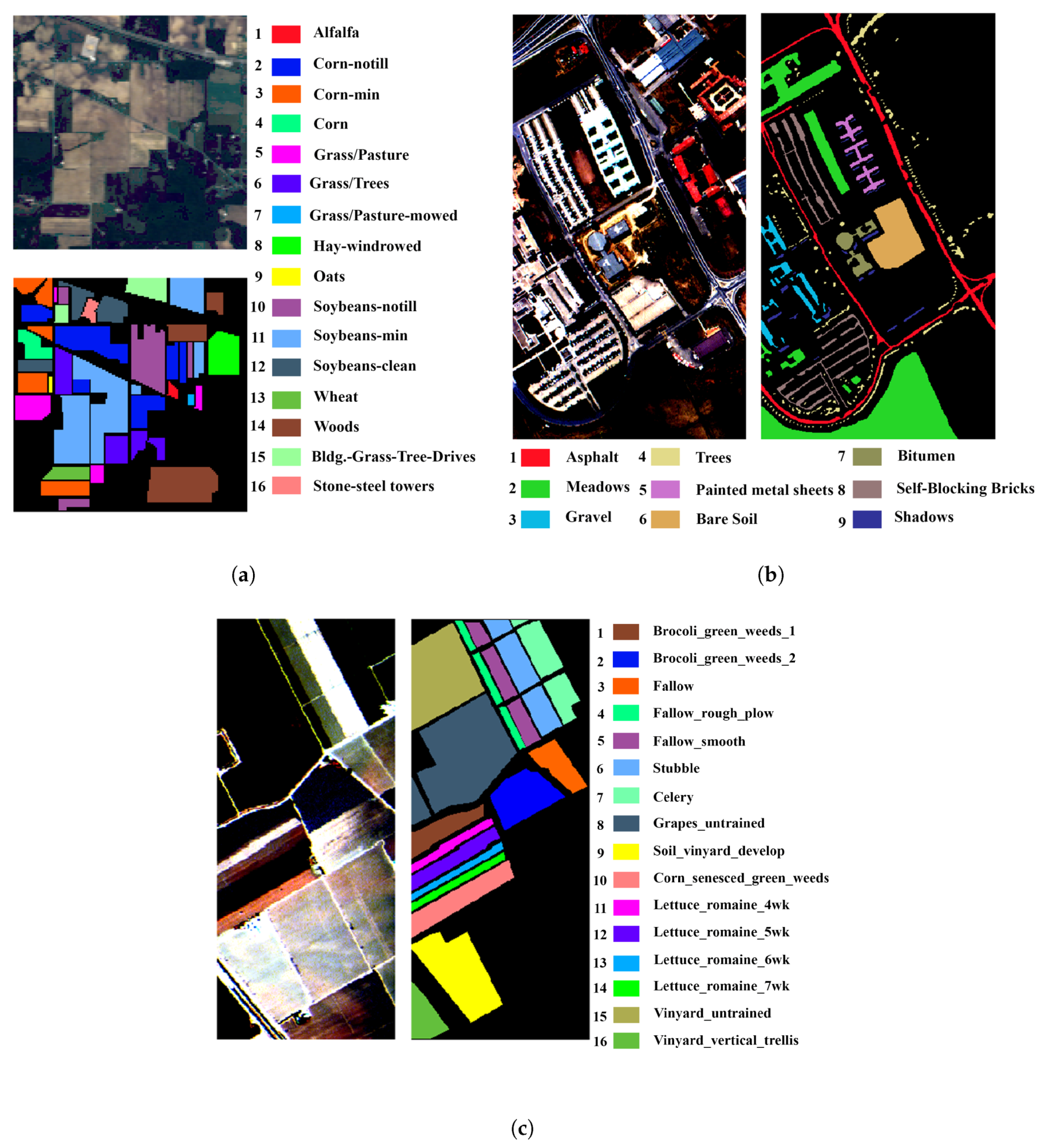
To comprehensively assess the performance of the proposed model, three different types of publicly available hyperspectral datasets, Indian Pines, University of Pavia, and Salinas, were chosen and are described next:
Indian Pines: The Indian Pines dataset (Indiana) was collected by Airborne Visible/Infrared Imaging Spectrometer (AVIRIS) over Northwestern Indiana in June 1992. This data includes 145 × 145 pixels in 220 spectral bands; however, 20 water absorption and low signal-to-noise bands were removed in our experiments. The spatial resolution of this data is 20 m, and the spectral bands cover wavelengths in the range of 0.4–2.5
m.
Figure 4a illustrates a false color composite and a ground truth map of the data. The ground truth map contains 16 land-cover classes, including the different types of vegetation species. For the training process, 30% of the labeled data was randomly chosen, and the rest was left just for the testing process.
Table 1 indicates the number of training and test samples for each class.
University of Pavia: The University of Pavia (PaviaU) dataset was captured by Reflective Optics System Imaging Spectrometer (ROSIS-3) over this Italian university’s engineering school in 2001. This dataset originally contained 113 spectral bands, with the size of 610 × 340 and a spatial resolution of 1.3 m. However, after removing noisy and damaged spectral bands, 103 bands in the range of 0.43–0.86
m remained.
Figure 4b shows a false color composite of the data and its ground truth map. The ground truth map contains nine different types of urban classes. As tabulated in
Table 2, 20% of the labeled samples were randomly selected for the training process, while the remaining samples were only used for the testing process.
Salinas: The Salinas dataset consists of 512 × 217 pixels, captured by the AVIRIS sensor over the Salinas Valley in California, USA, in 1992. After removing noisy spectral bands, 204 bands, each with the spatial resolution of 3.7 m, were used in our experiments. As shown in
Figure 4c, sixteen classes related to different agricultural crops were collected in the ground truth map. According to
Table 3, about 18% of the labeled samples were used for the training, and the rest were considered completely for the testing.
3.2. Experimental Settings
To comprehensively qualify the performance of the PRCLSTM model, four classification metrics, namely Overall Accuracy (OA), Kappa Coefficient (), Average Accuracy (AA), and Test Error (TE), are used in this study. The first three classification metrics are extracted from the confusion matrix, whereas the last one is the expected value of error on a new input of the network. This last criterion indicates the generalization capacity of the model, and its lower value demonstrates a better performance. To assess the independency of the proposed model on training and test data distributions, all experiments are repeated ten times with a random train and test splitting. Finally, the average and the standard deviation of the experiments are estimated and reported.
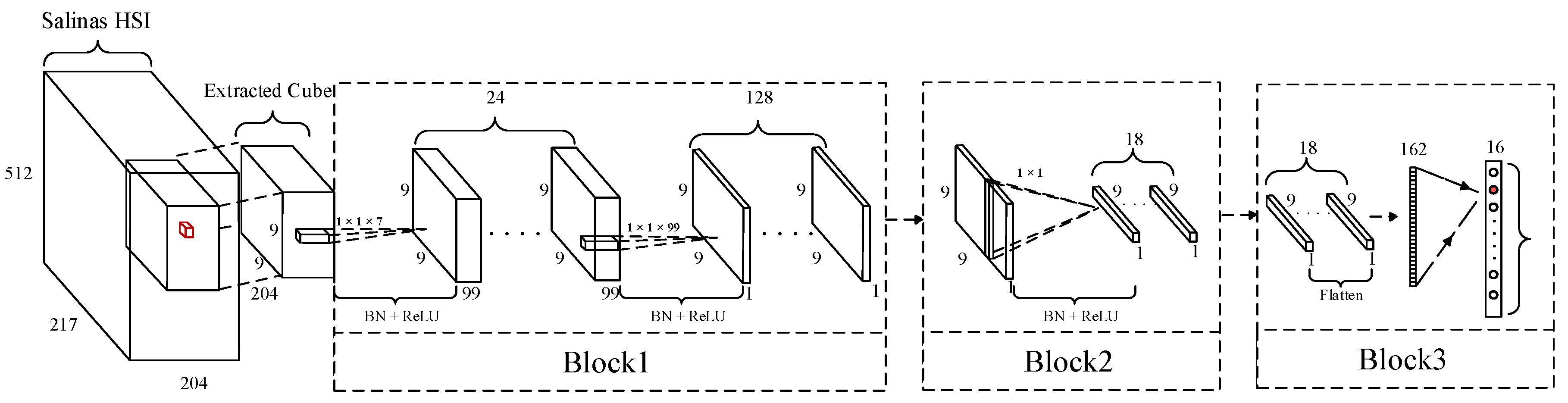
Before discussing the parameter setting for the proposed model, we show the model’s framework and configuration for the Salinas dataset in detail (
Figure 5 and
Table 4). Inspired by Reference [
27], we set the parameters of Block 1. To do so, the number of filters of CNN1 and CNN2 are respectively considered as 24 and 128 in this block. At the same time, the kernel sizes of CNN1 and CNN2 are also respectively set as
and
, where
K is the third dimension of the output of the previous layer. In Block 2, to completely use the spatial information of an input cube, the kernel size of the CLSTM layer is set to
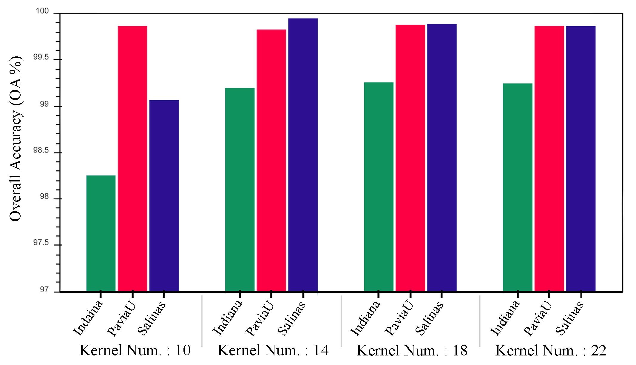
. To set the number of outputs of Block 2, the different number of kernels in the range of 10 to 22 with a step size of four are assessed. As illustrated in
Figure 6, the model with 18 kernels has the higher mean of OA in the datasets in question. Thus, we choose this number for the output of Block 2 in our proposed model.
In the second part, the optimal parameters for the training process, specifically the batch size and learning rate, are obtained via a grid search algorithm. Note that the search space of these two parameters is set to References [
16,
27,
29,
45,
46]. As a result of the grid search, the learning rate was set to 0.0001, 0.0003, and 0.0001 for Indiana, PaviaU, and Salinas, respectively. We also consider 0.00001 as the learning decay only for PaviaU because this parameter does not show a positive effect on the other datasets. The batch size is also set to 16 for all the experiment datasets.
In the third part, we set the parameters of the regularization techniques. In the PRCLSTM model, two types of regularization techniques—Batch Normalization (BN) [
34] and dropout [
47]—are taken into account. As already mentioned, BN is used to tackle the internal covariant shift phenomenon [
34], and the dropout is applied to increase the generalization capacity. Accordingly, BN is applied to the fourth dimension of each layer output to make the training process more efficiently. In addition, according to the number of the inputs, 30% of the connections and nodes are discarded by a dropout method for the CLSTM layer. Through the dropout method, 50% of the nodes are ignored in order to prevent overfitting in the classification layer. Finally, in the last part, we initialize the kernels of the CNN and CLSTM layers by using the truncated normal distribution [
48]. Then, these initial values are optimized using a root mean squared error propagation (RMSProp) [
49] as an optimizer to back propagate the gradient of the categorical cross-entropy cost function. In the training phase, after each epoch, the trained model is evaluated by the validation set, and the model with the lowest TE is preserved. Subsequently, the obtained model is applied for the testing procedure which provides the evaluation results.
3.3. Competing Methods
In order to evaluate the performance of the PRCLSTM, the model is compared to different types of classifiers like SVM, 1-D, 2-D, and 3-D CNN and RNN. Moreover, to analyze the effect of spectral-spatial feature extraction blocks, two additional models are also implemented. The configurations of the competing methods are as follows:
P-SVM-RBF: an SVM classifier with an radial basis function (RBF) kernel used to estimate class membership probabilities by an expensive K-fold cross-validation.
P-CNN [
50]: a 2-D CNN layers with a PCA as a preprocessing procedure.
CRNN [
31]: 1-D CNN layers, followed by two fully connected RNN layers.
3-D-CNN [
51]: 3-D CNN layers, followed by fully connected layers.
3-D-CNN-LSTM: Our proposed model in which a CLSTM layer is replaced with a fully connected LSTM. This model was performed to demonstrate the efficacy of Block 2.
L-CLSTM: Our proposed model in which all layers are replaced with the CLSTM (L-CLSTM is the long CLSTM). This model was implemented to indicate the Block 1 efficiency.
To evaluate the performance of PRCLSTM, as a 3-D-LSTM-based model, we first compare that to two implemented 3-D-LSTM-based models, namely 3-D-CNN-LSTM and L-CLSTM. These models are then comprehensively compared with the other competitive classifier methods (cases 1–4 above). The best results based on the four classification metrics have been bolded in the different tables.
3.4. Analyses of the 3-D-LSTM-Based Models
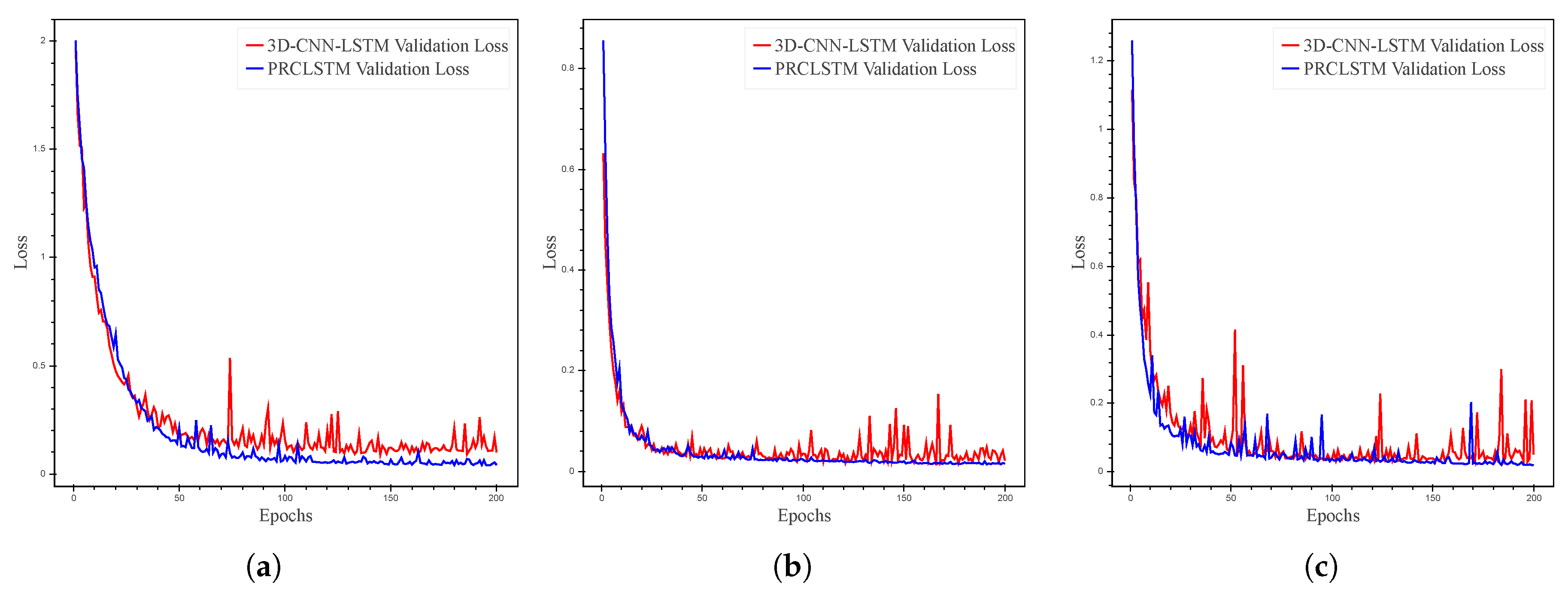
In the first phase, the effect of Block 2 is analyzed through a comparison of 3-D-CNN-LSTM and PRCLSTM.
Figure 7 illustrates the performance of the two models in terms of the validation loss (validation error) during the training process for the Indiana, PaviaU, and Salinas datasets. As is clear from
Figure 7, the performance of the PRCLSTM is more stable than that of the 3-D-CNN-LSTM model. Moreover, our model, having a CLSTM layer, converges to a far better solution than that of the 3-D-CNN-LSTM. According to the test results (
Table 5,
Table 6 and
Table 7), compared with the 3-D-CNN-LSTM, the PRCLSTM leads to 0.98%, 1.14%, 2.48%, and 0.05 improvements in the OA,
, AA, and TE respectively, averaged on all three datasets. For example, the improvements for Indiana in terms of OA,
, AA, and TE have respectively been 1.73%, 1.98%, 6.16%, and 0.08. In addition, as is obvious from the classification maps in
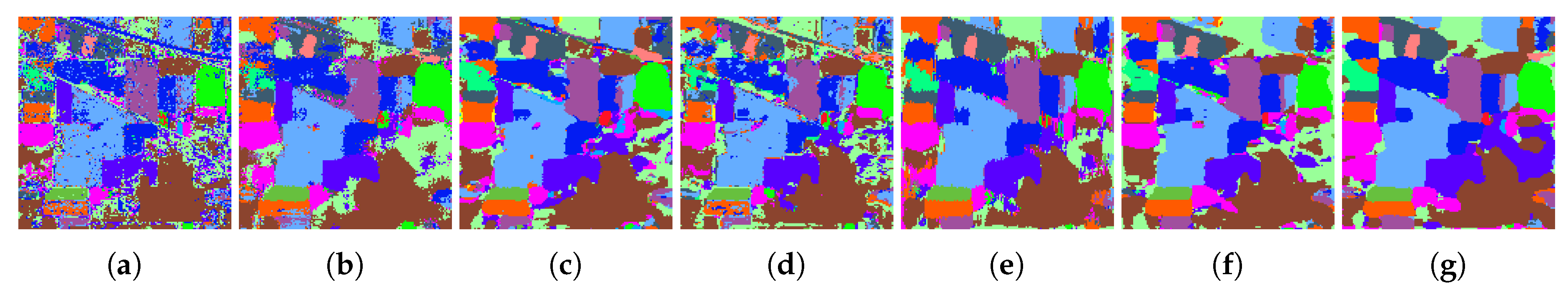
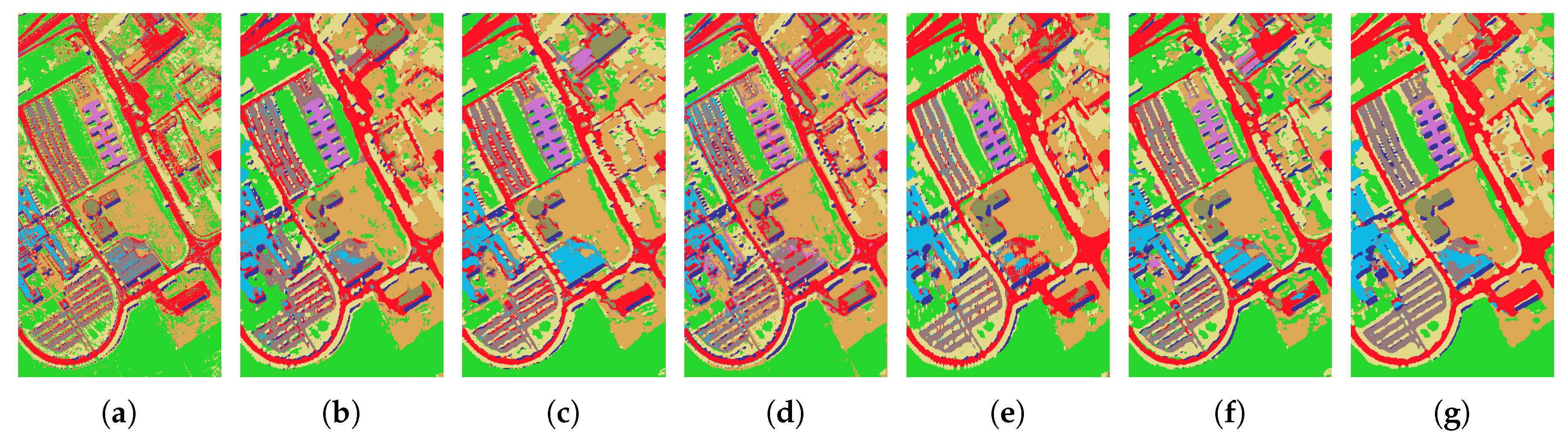
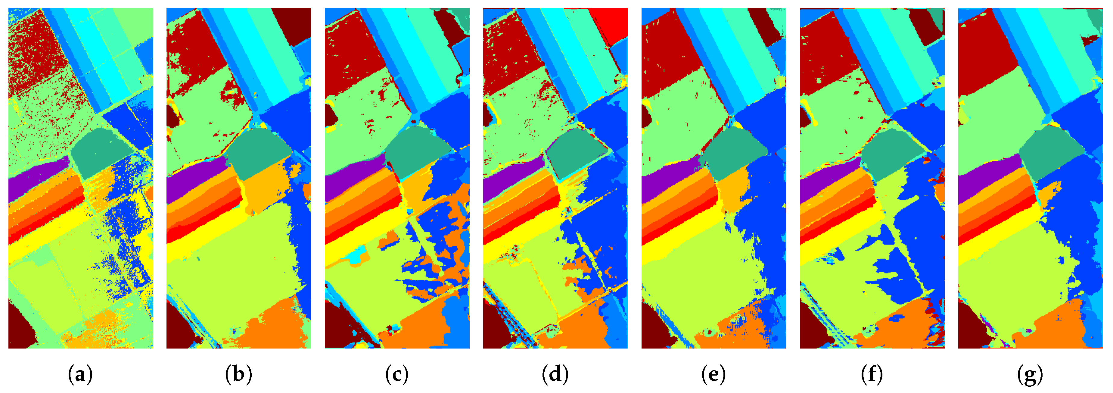
Figure 8,
Figure 9 and
Figure 10, the 3-D-CNN-LSTM, unlike our proposed model, leads to a great deal of noise and a malicious effect, both from the flatting out of the 3-D data by the fully connected LSTM layer for the PaviaU dataset and, especially, for the Indiana and Salinas datasets. As our experimental results indicate, considering the spatial information of data during sequence-based prediction leads to a more-effective learning process.
The second phase analyses the effect of the spectral feature extraction and dimension reduction, performed by the 3-D-CNN layers in Block 1. For this purpose, the L-CLSTM model, which contains only CLSTM layers, is selected. To achieve a fair comparison, the parameters of the L-CLSTM model are considered to be approximately equal to the PRCLSTM model. As illustrated in
Figure 11, due to the high dimension of the input data, the L-CLSTM model, unlike the PRCLSTM model, cannot converge to the proper solution in terms of the validation loss during the training process for any of the datasets.
Table 5,
Table 6 and
Table 7 show that the PRCLSTM leads to on average 1.91%, 2.24%, 1.51%, and 0.09 improvements in the OA,
, AA, and TE, respectively, for all of the three datasets compared to L-CLSTM. From the perspective of computational burden, as seen in
Table 8, the computational cost of the L-CLSTM model is much higher than that of the PRCLSTM model. The results in this phase imply that the extraction of low-dimensional shallow features, as inputs of Block 2, play a key role in improving the performance of the recurrent analysis.
3.5. The PRCLSTM Performance
The two main factors that influence the performance of DL methods in an HSI classification task are the spatial size of an input cube and the number of training samples. Accordingly, we establish a three-part analysis to evaluate the performance of the proposed model in terms of these parameters. In the first part, the performance of the models is assessed in the presence of a fixed and sufficient number of training samples, as well as a fixed spatial size for the input cube. To do so, the training and test samples are determined as reported in
Table 1,
Table 2 and
Table 3. To prevent over-fitting and to enhance the training procedure, 35%, 50%, and 50% of the training samples are selected for the validation of the learned parameters of Indiana, PaviaU, and Salinas, respectively, during the training process. It is worth mentioning that the test samples are involved in neither the validation nor the training procedures and that they are just used for testing. The hyper-parameters of the 3-D-CNN-LSTM and L-CLSTM models are set the same as the PRCLSTM model, and for the other models, these parameters are set based on their original implementations. To have a fair comparison, a
(
B is the number of spectral bands) window size is selected as the input cubes of all models, and 200 is set as the number of training epochs. The results of the evaluation criteria for all models in hand have been illustrated in
Table 5,
Table 6 and
Table 7 for the Indiana, PaviaU, and Salinas datasets, respectively. These tables demonstrate that the PRCLSTM model achieves the best performance in all three datasets. For instance, in the Indiana dataset, the PRCLSTM achieves about a 2% higher accuracy in terms of the OA as well as a standard deviation three times lower than the best result gained by the other competitors. Moreover, according to
Figure 8,
Figure 9 and
Figure 10, the PRCLSTM produces the most accurate and noiseless classification maps.
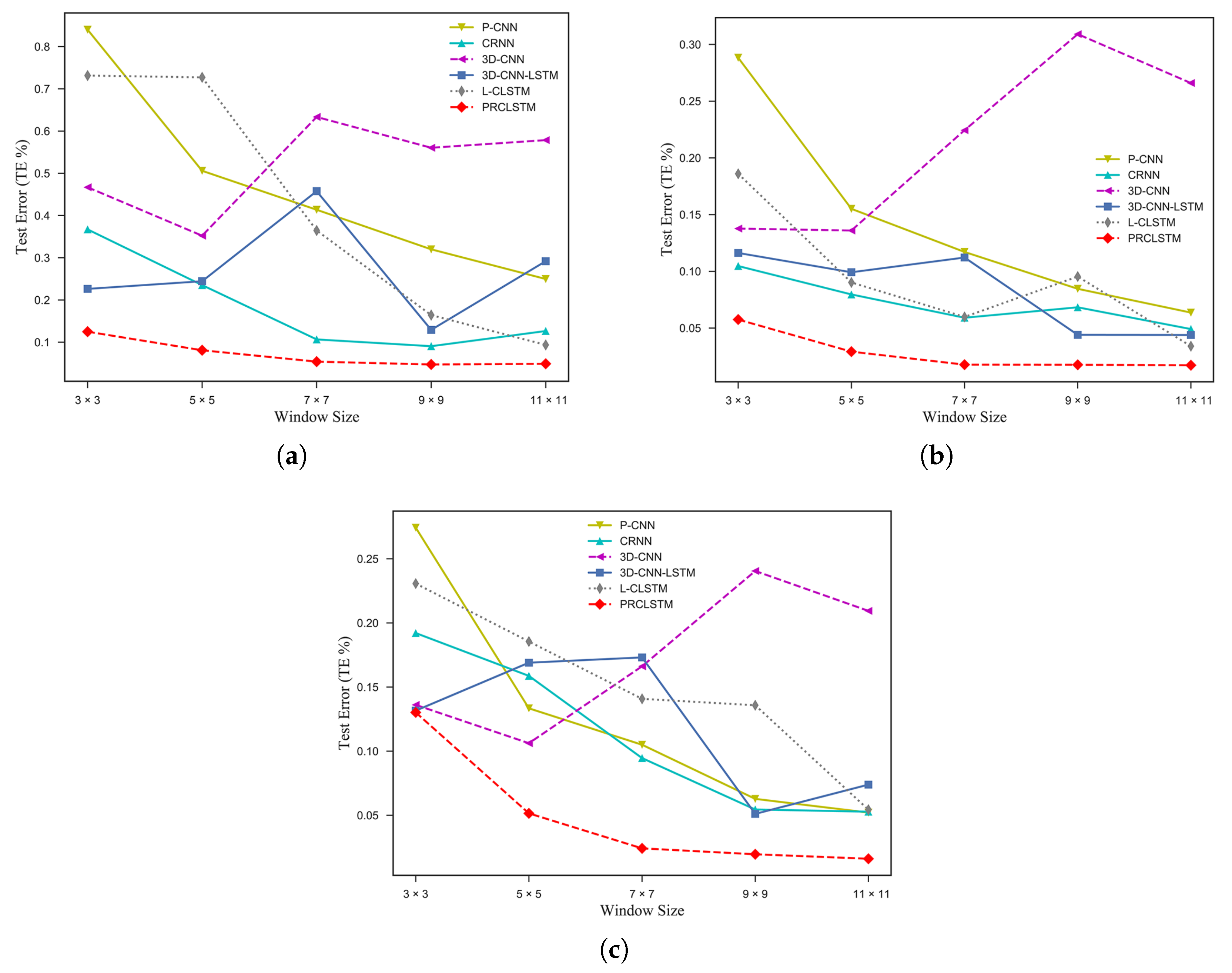
In the second part, the training processes with different spatial sizes of input cubes are performed. We set the extracted window to a range of sizes from
to
and report the OA and TE for each model.
Table 9 and
Figure 12 indicate that the proposed model achieves the best results in most cases. However, for the Salinas dataset, the 3-D-CNN-LSTM performs relatively better than the PRCLSTM in terms of the OA for the
window size, but the PRCLSTM still shows the lowest TE, guaranteeing a better generalization capacity for our model. These results indicate that the proposed model performs better in the various sizes of input cubes compared to the convolutional feed-forward-based models, thanks to the use of a convolutional recurrent structure to capture the spatial information of data. For example, the 3-D-CNN model, as a competing method, performs the best in the case of the
window size, whereas its performance deteriorates for the other window sizes.
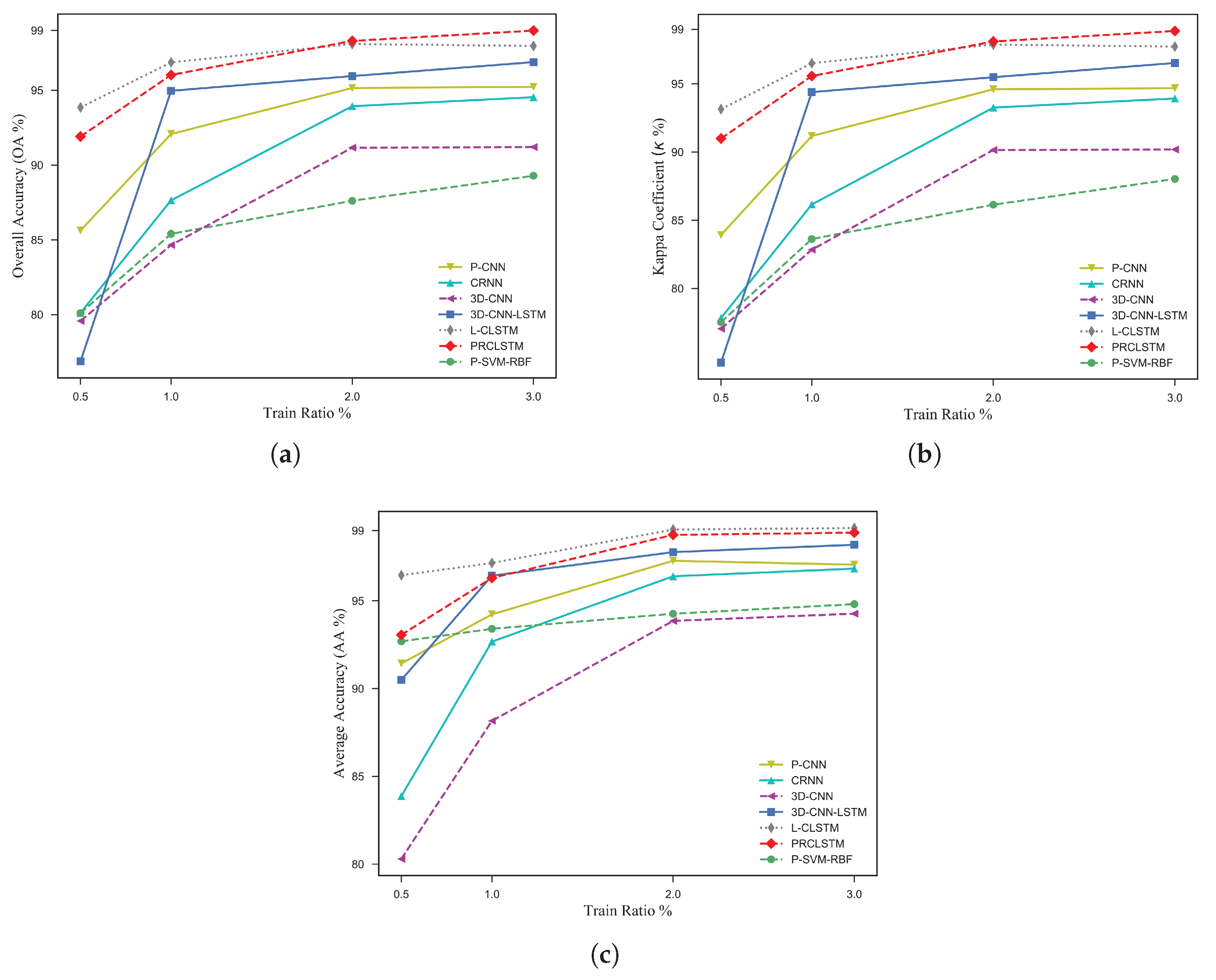
In the third part, we assess the capability of the proposed model when a small amount of training data is available. For this purpose, the Salinas dataset is selected and the models are trained by a range of 0.5% to 3% of data as training samples. Then the OA,
, and AA are reported for the rest of the samples. From the experiments, first of all, one can conclude that the models which contain a convolutional recurrent unit perform better than the models with a convolutional feed-forward unit when limited training samples are accessible. For example, as is obvious from
Figure 13, where the competing methods, such as the CRNN and 3-D-CNN, lead to about an 80% accuracy in terms of the OA, the convolutional recurrent models, that is, the PRCLSTM and L-CLSTM, result in a higher than 91% accuracy. It should be noted that, in the case of very limited training samples (i.e., 0.5% and 1%), the L-CLSTM model results in a relatively higher classification accuracy; however, this improvement is not reliable because the accuracy of the L-CLSTM fluctuates with an increase in the number of training samples. Generally speaking, the results of the PRCLSTM are more accurate and more stable in both scenarios of having sufficient and limited training samples.
In addition to the abovementioned analyses, the training and testing time of the 3-D-LSTM model for the constant spatial size of the input cubes (i.e.,
) and a sufficient amount of training samples are tabulated in
Table 8. Thanks to the Graphical Processor Unit (GPU) resources, the computational cost of DL methods is reduced. In general, recurrent-based models are still computationally expensive; however, as observed in
Table 8, two 3-D-LSTM-based models (3-D-CNN-LSTM and PRCLSTM), by taking advantage of the dimensionality reduction of the 3-D CNN are able to reduce the computational burden of CLSTM. Furthermore, to statistically compare the proposed method with its best rivals in each dataset, the wilcoxon rank sum test [
52] was used here. This test, which is a common statistical test, can be applied to compare two independent sets of samples without having any assumption about the statistical distribution of the sets. In our case, a set is a 10 × 1 vector of
values, coming from 10 runs of each classifier. The obtained result, tabulated in
Table 10 indicates that the differences between PRCLSTM and the competing models are statistically significant at the confidence level of 95%.
4. Conclusions
In recent years, deep learning (DL) methods are of major concern in hyperspectral imagery (HSI) classification tasks. These methods are able to automatically extract spectral and spatial information and to apply them in classification processes. However, a full extraction of both the spectral and spatial information are the main concerns of these methods. To address them, here, an innovative convolution-recurrent framework has been presented to build a 3-D spectral-spatial trainable model for HSI classification. This model contains two stages: (i) the 3-D CNNs, which produce shallow spectral-spatial features in a feed-forward procedure, and (ii) a CLSTM, which extracts more abstract and semantic features in a recurrent manner. The focus of the first stage is to analyze a high spectral dimension, while the concentration of the second one is to process the full content of spatial information. In this study, the performance of the PRCLSTM (the proposed model) has been assessed in the presence of (i) a sufficient number of training samples, (ii) a limited number of training samples, and (iii) different input cubes sizes. From the results, it can be concluded that the PRCLSTM performance is promising, even with a limited number of training samples. Moreover, the recurrent analysis for extracting spatial information makes the classification model robust against the different input cubes sizes, indicating a high generalization capacity of the proposed model.


