Evaluation and Analysis of the Seasonal Cycle and Variability of the Trend from GOSAT Methane Retrievals

 , , , , ,
  , , , , , , , and
Abstract
:
1. Introduction
2. Data Description
2.1. GOSAT
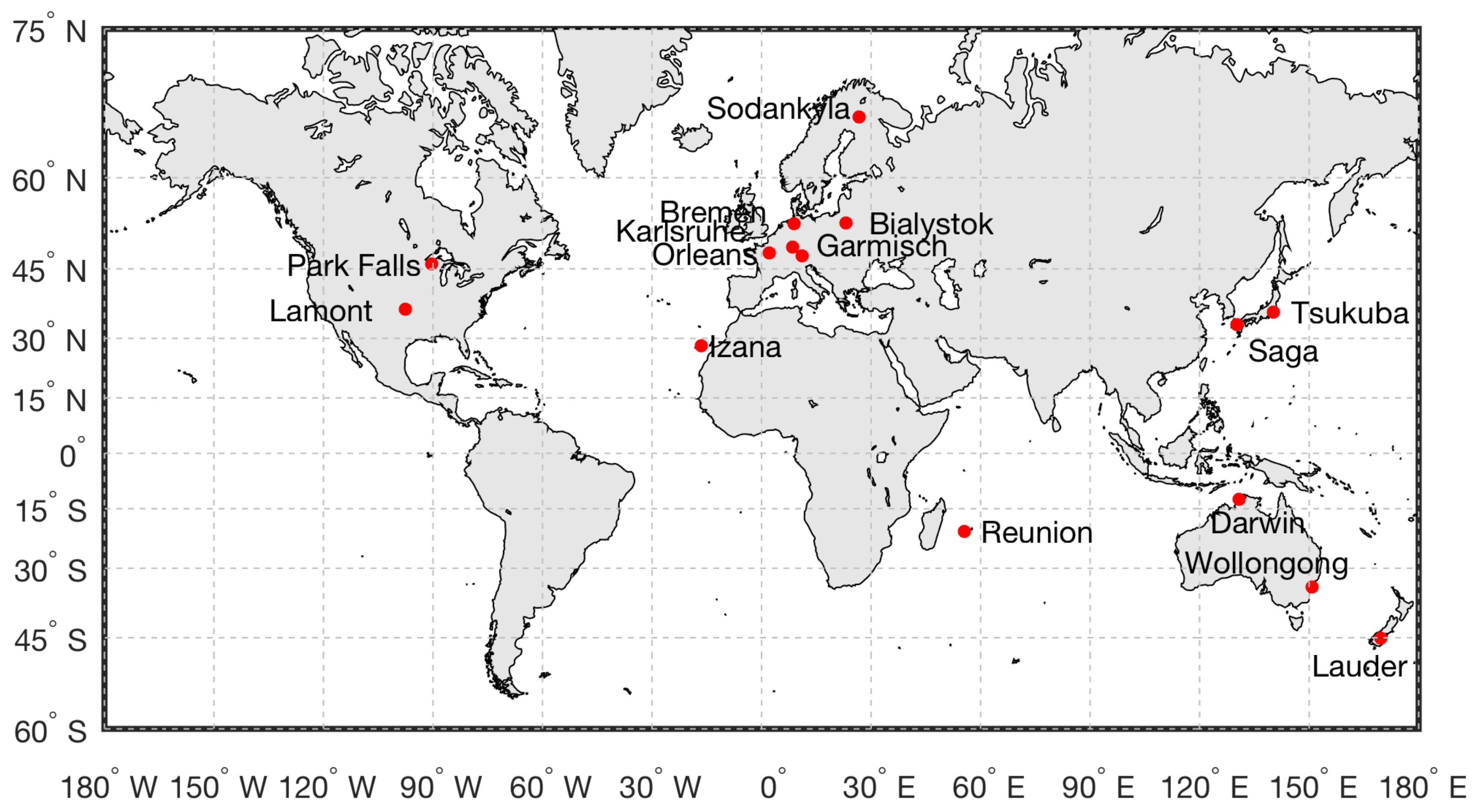
2.2. TCCON
2.3. NOAA Marine Boundary Layer Reference
2.4. CarbonTracker Europe–CH4
3. Methods
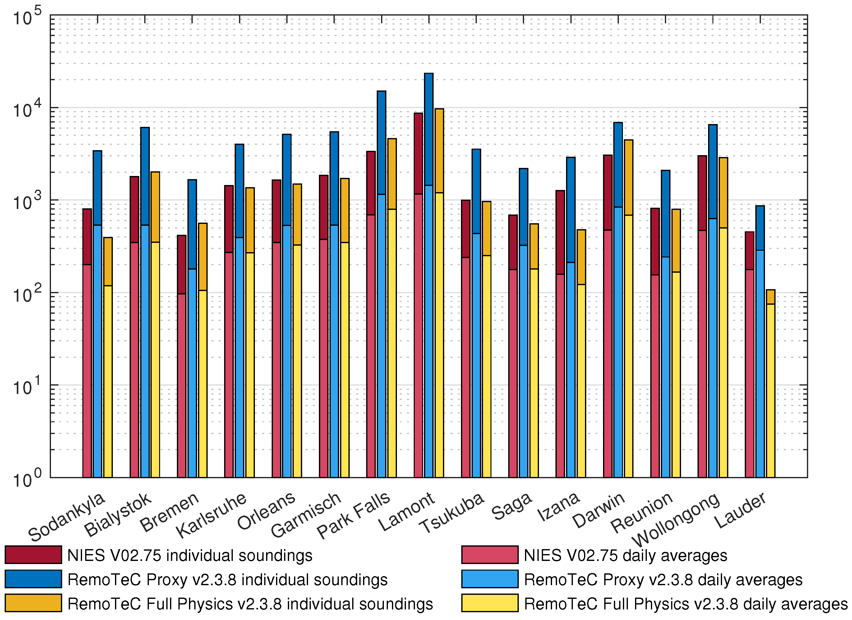
3.1. Co-Locating GOSAT and TCCON
3.2. Data Processing
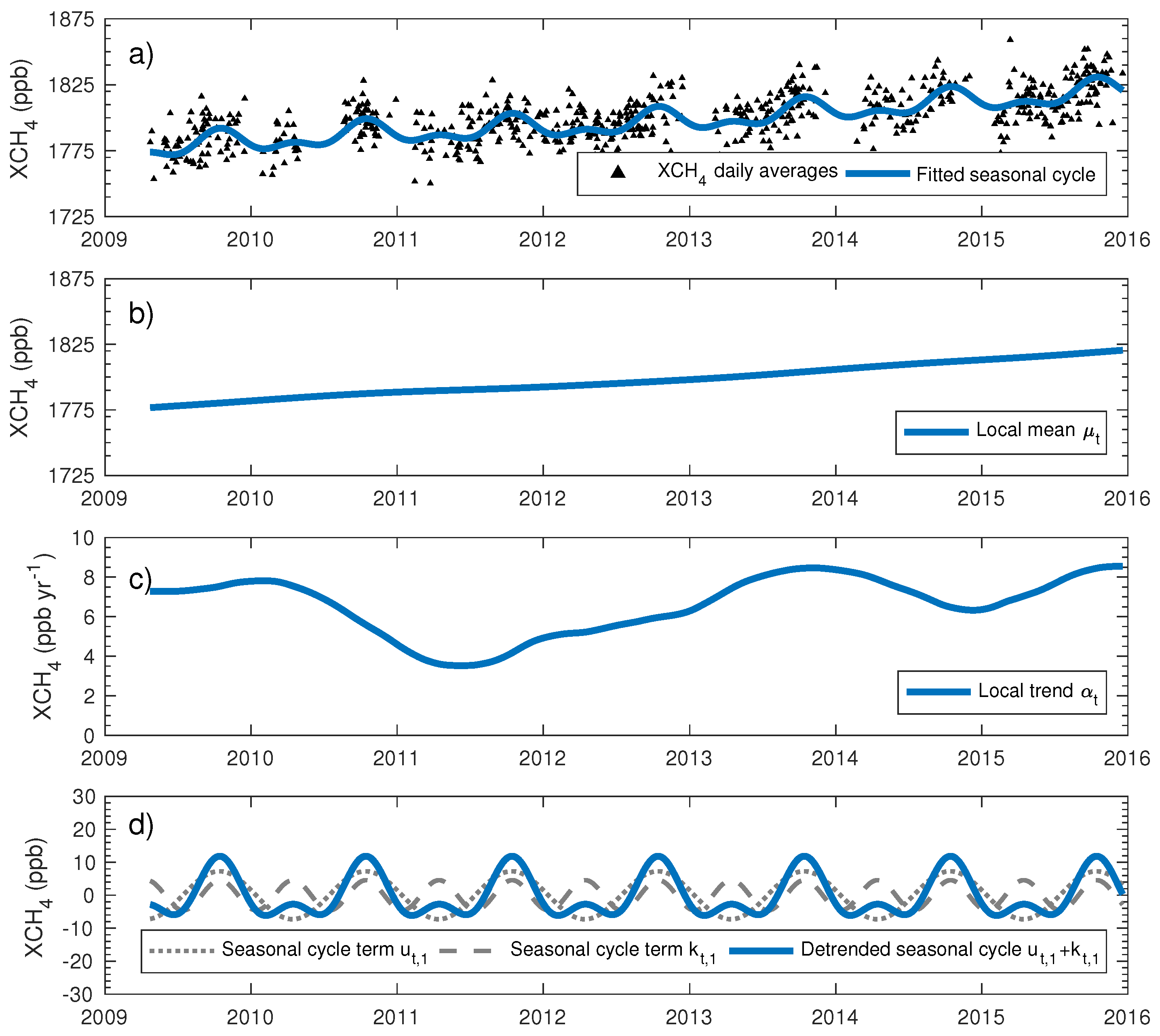
3.3. Seasonal Cycle and Trend by the DLM Approach
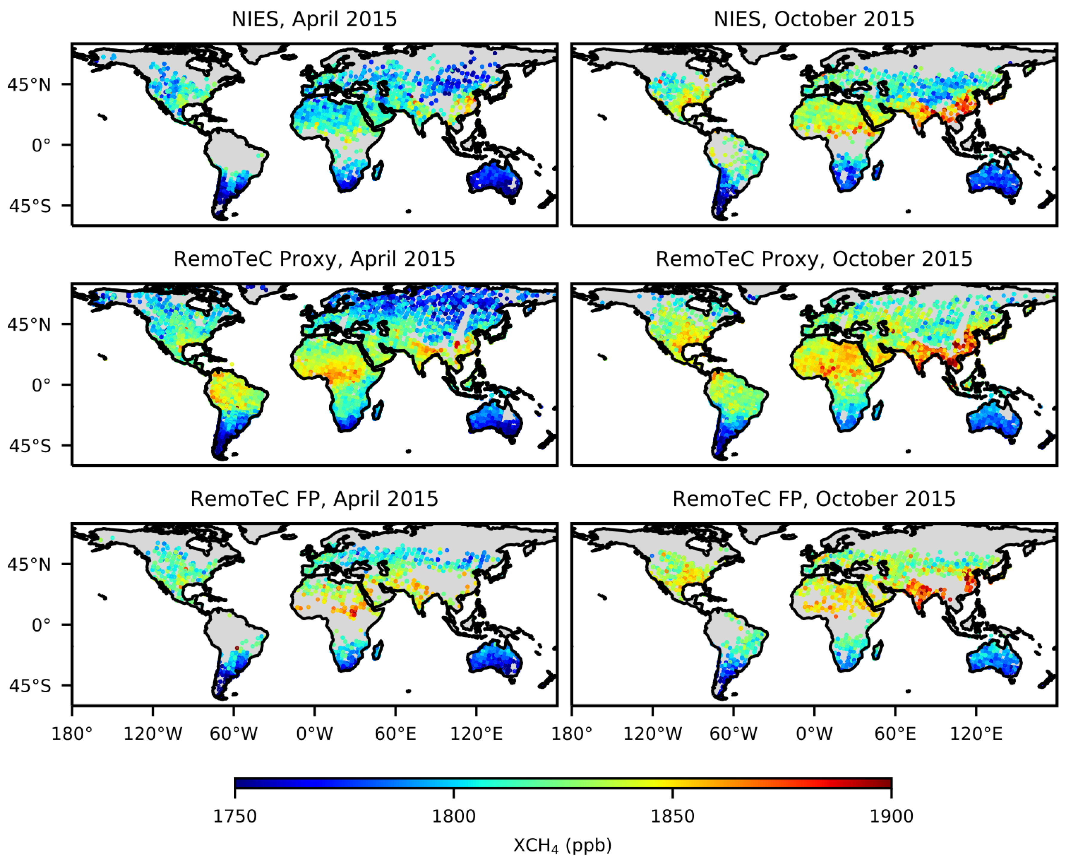
4. Results and Discussion
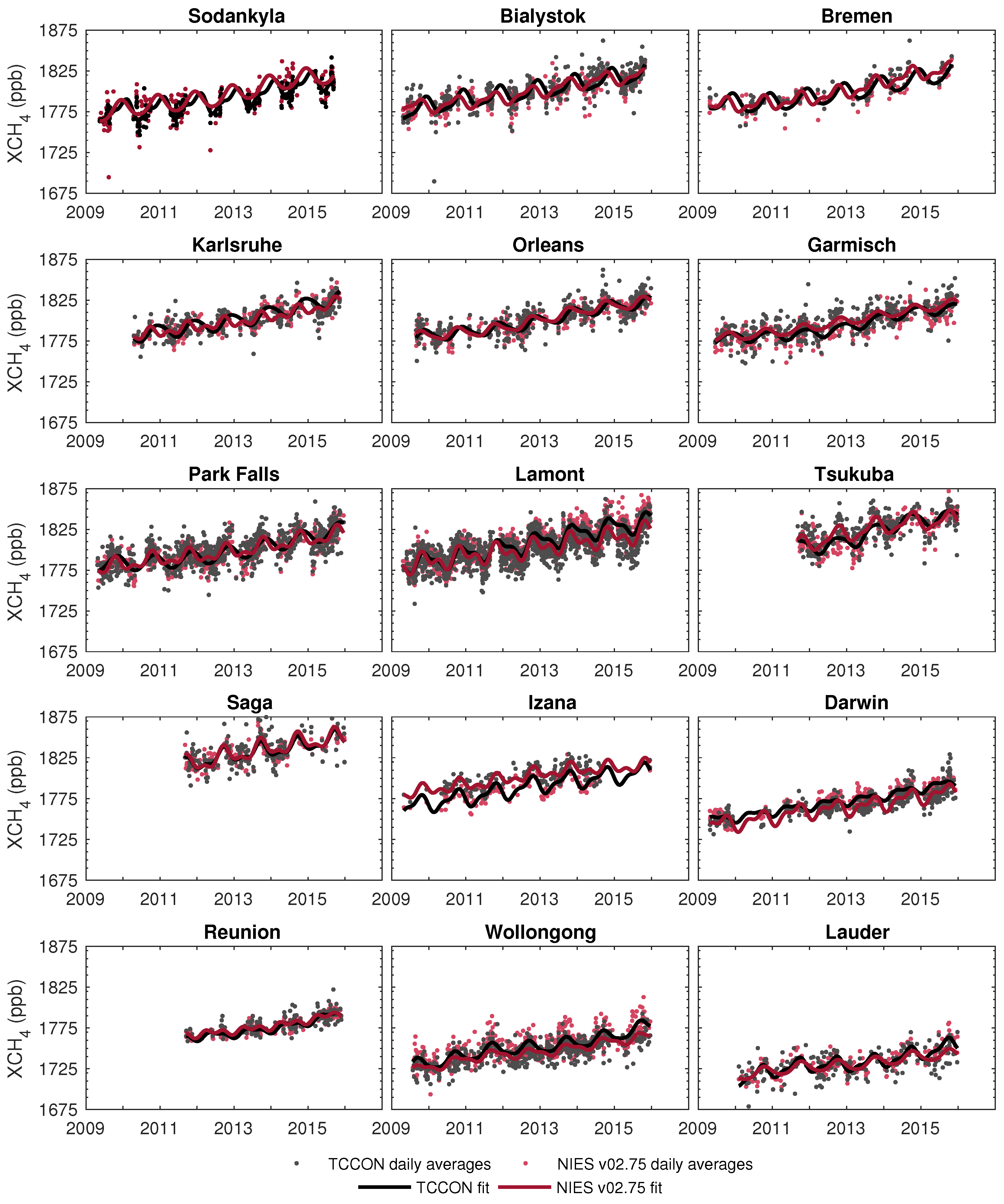
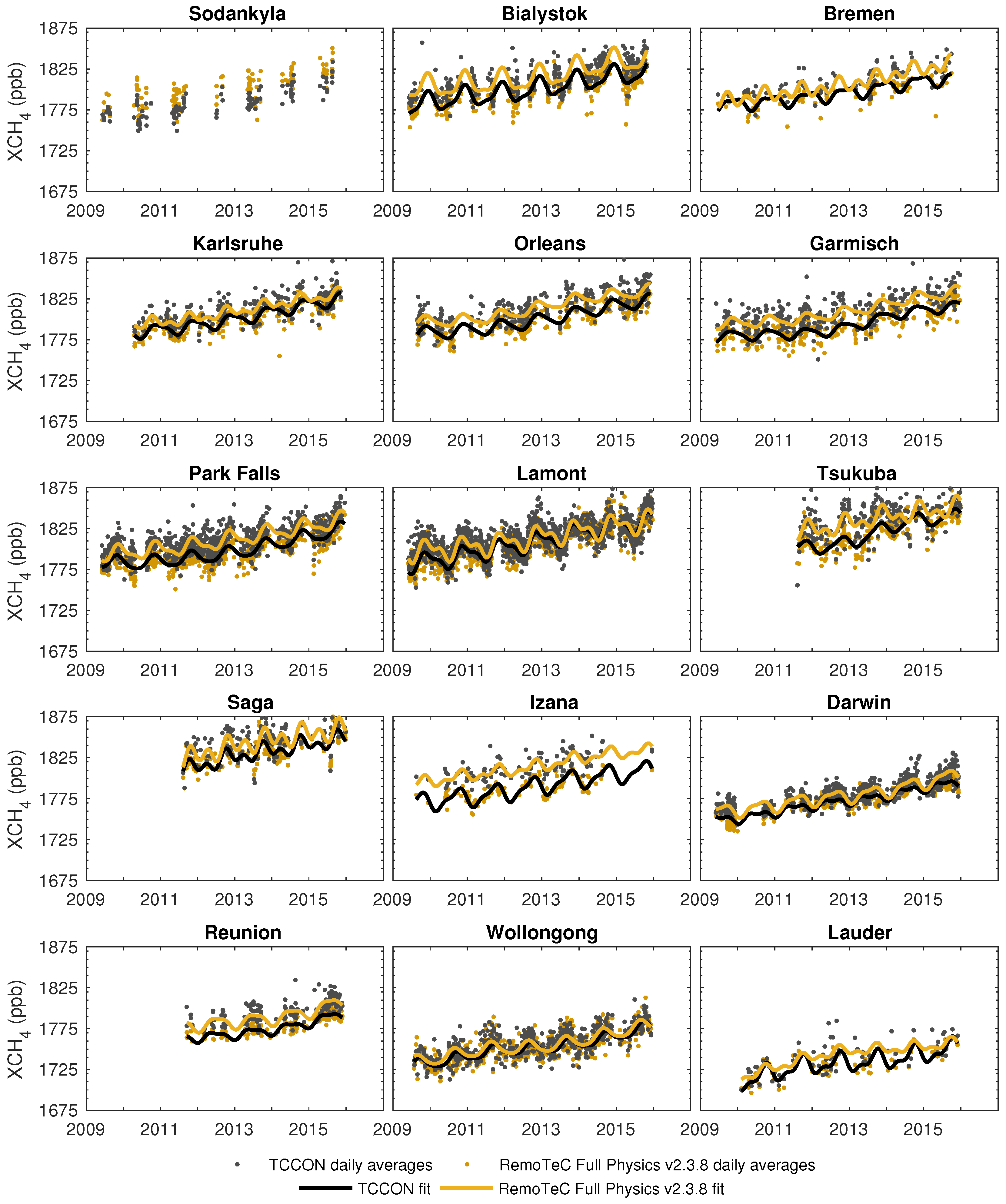
4.1. Evaluation Against TCCON
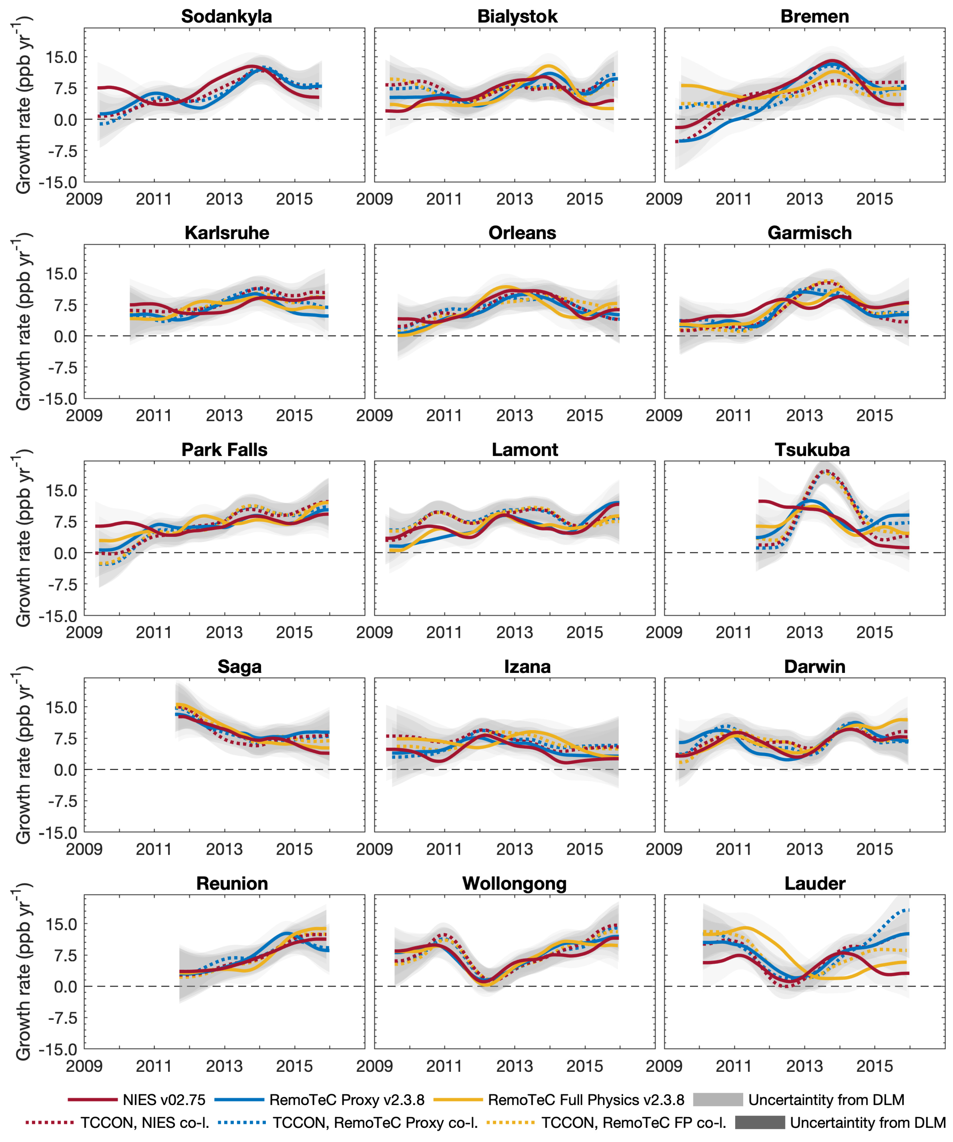
4.1.1. XCH4 Growth Rate
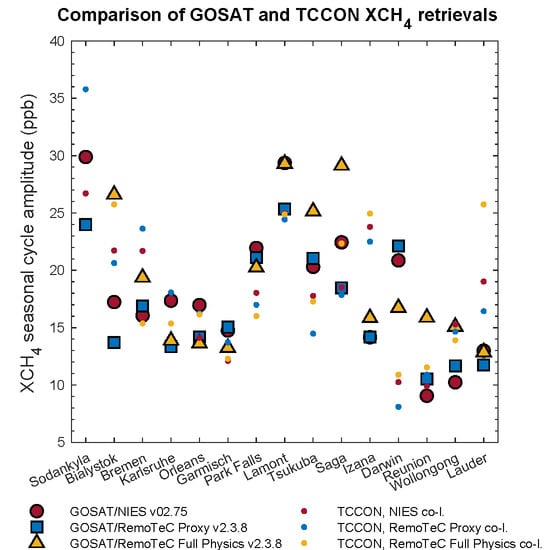
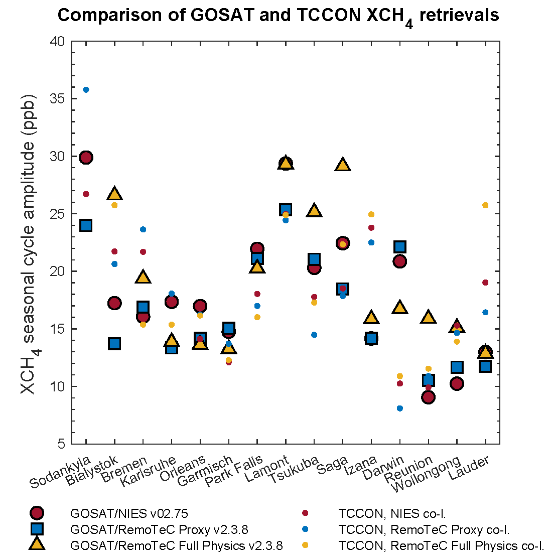
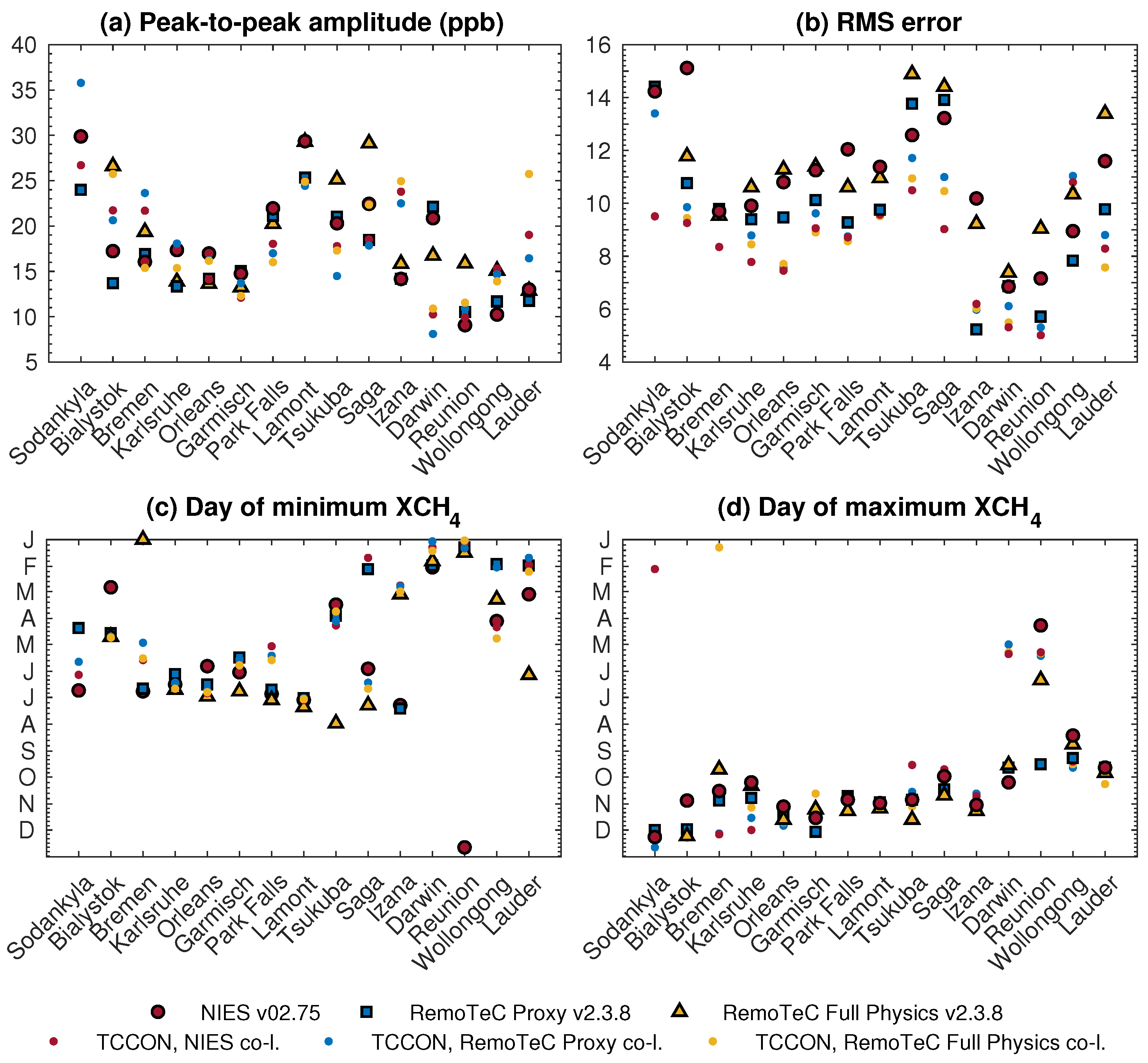
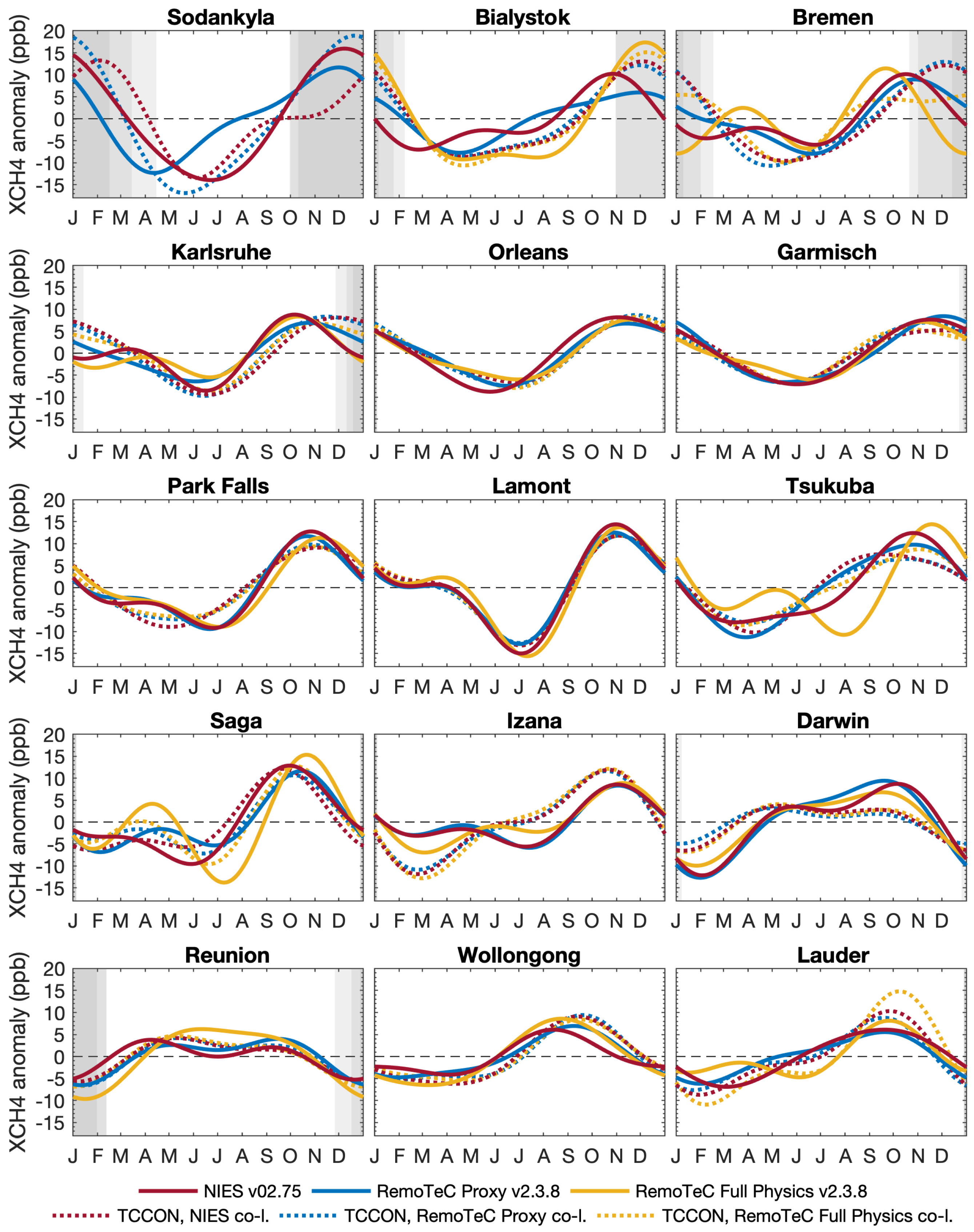
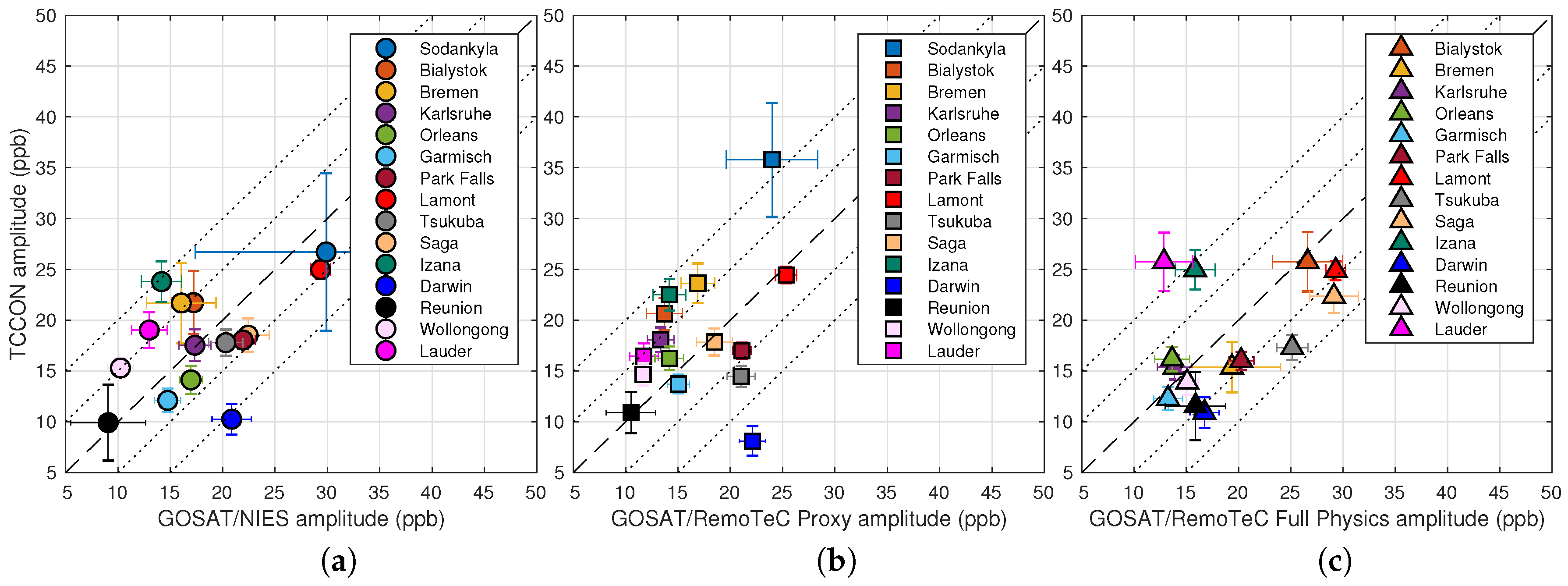
4.1.2. XCH4 Seasonal Cycle Amplitude
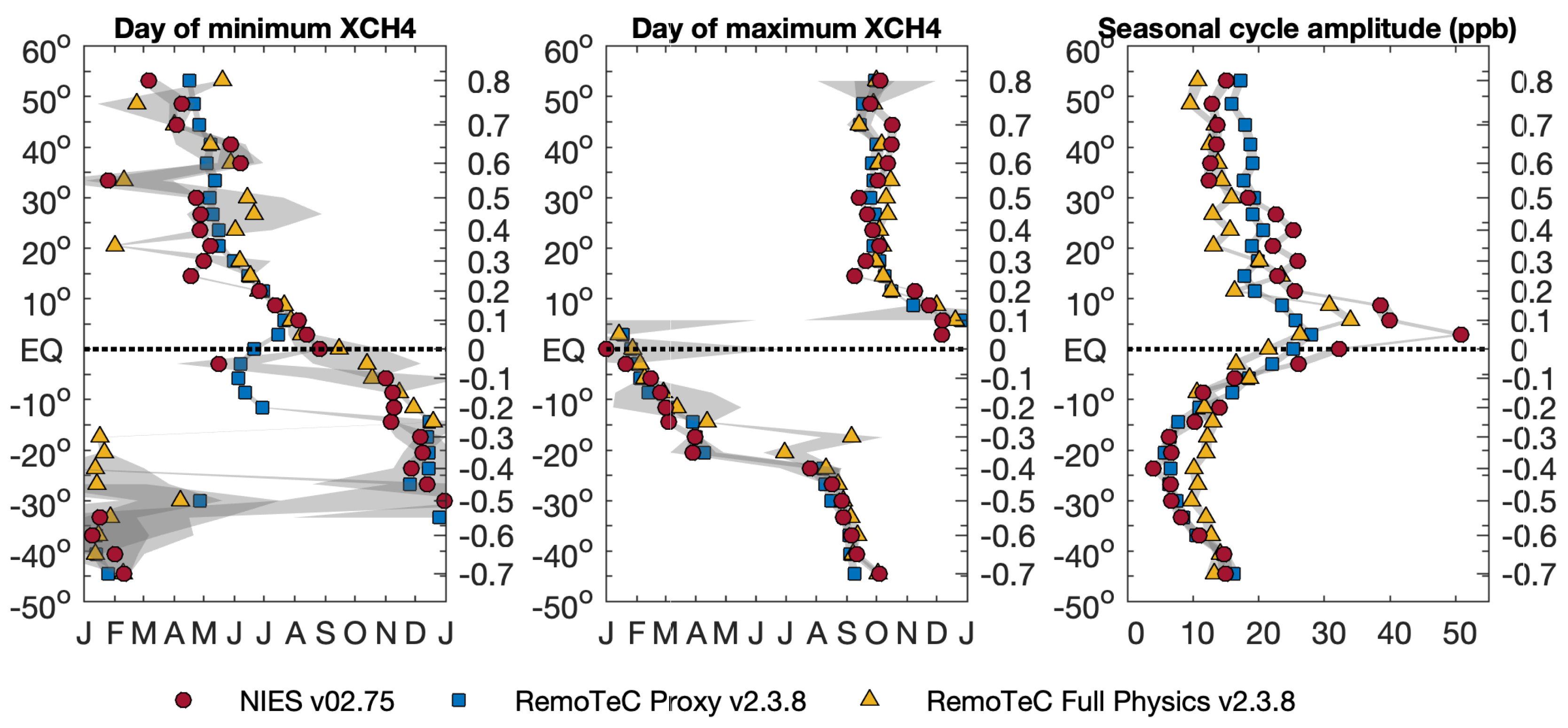
4.1.3. Phase of the XCH4 Seasonal Cycle
4.1.4. Considering the Sources of Uncertainties
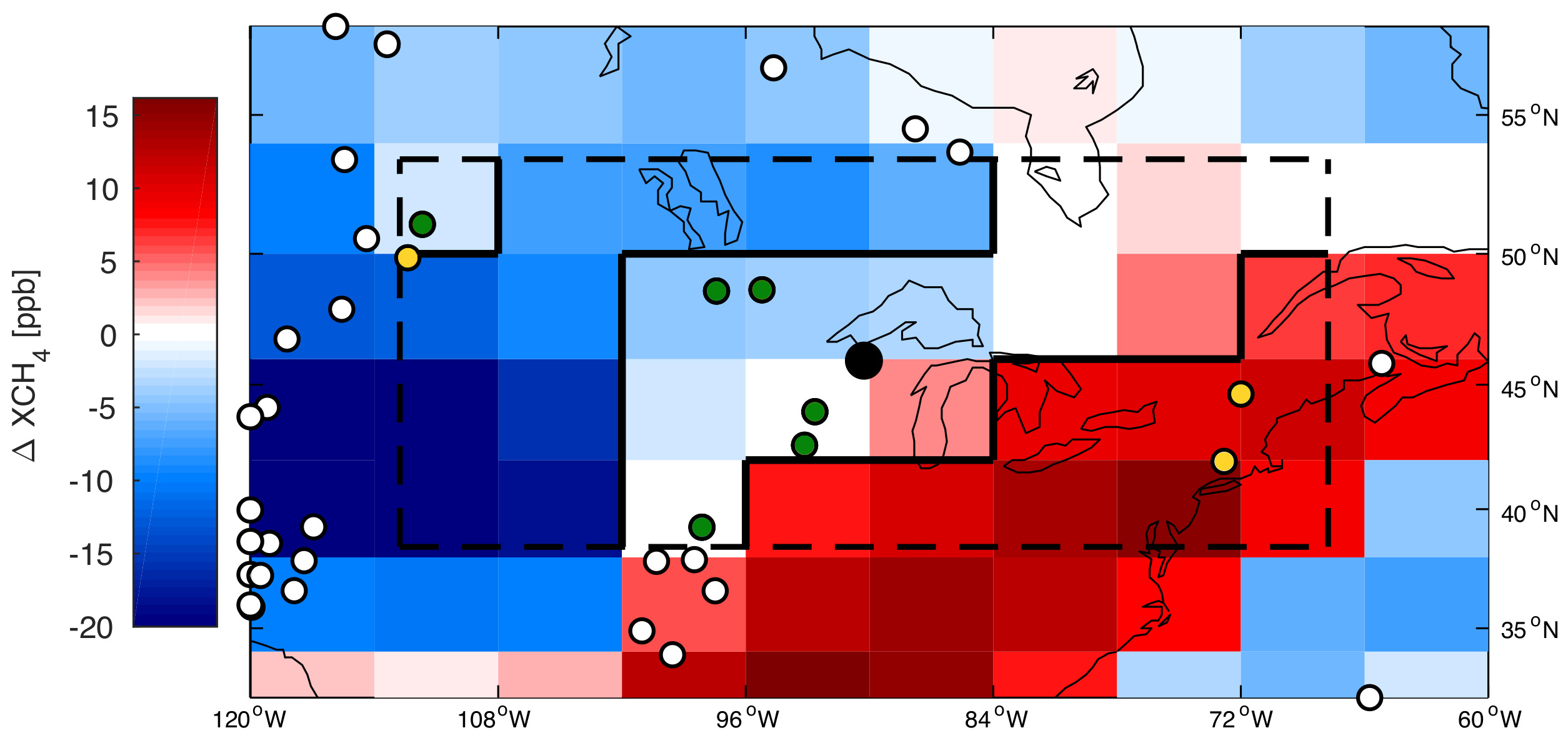
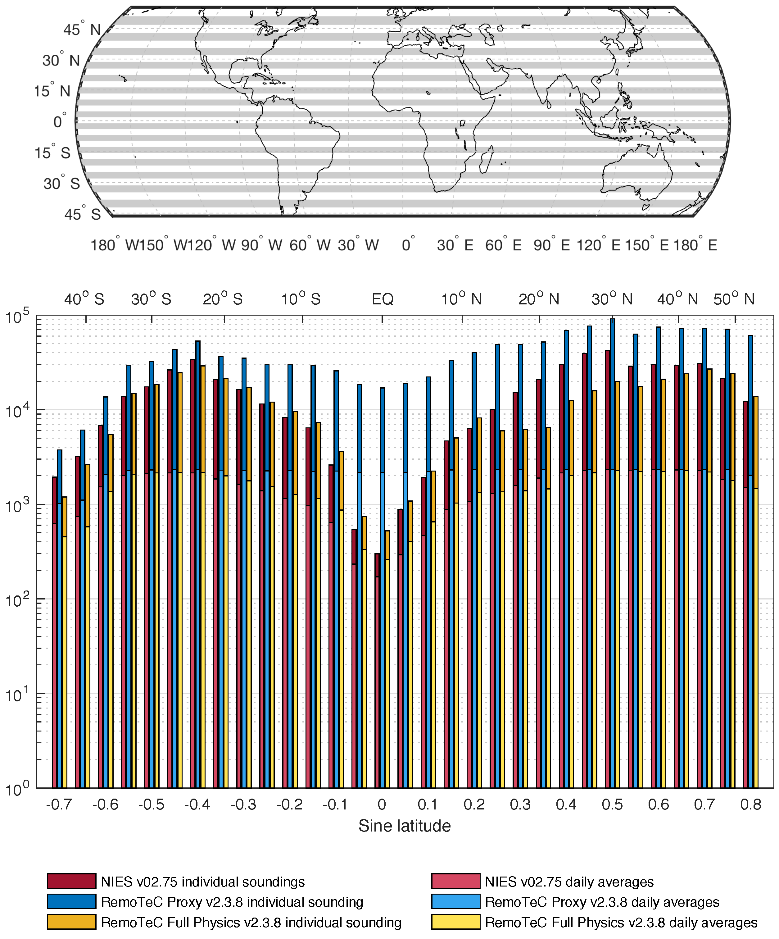
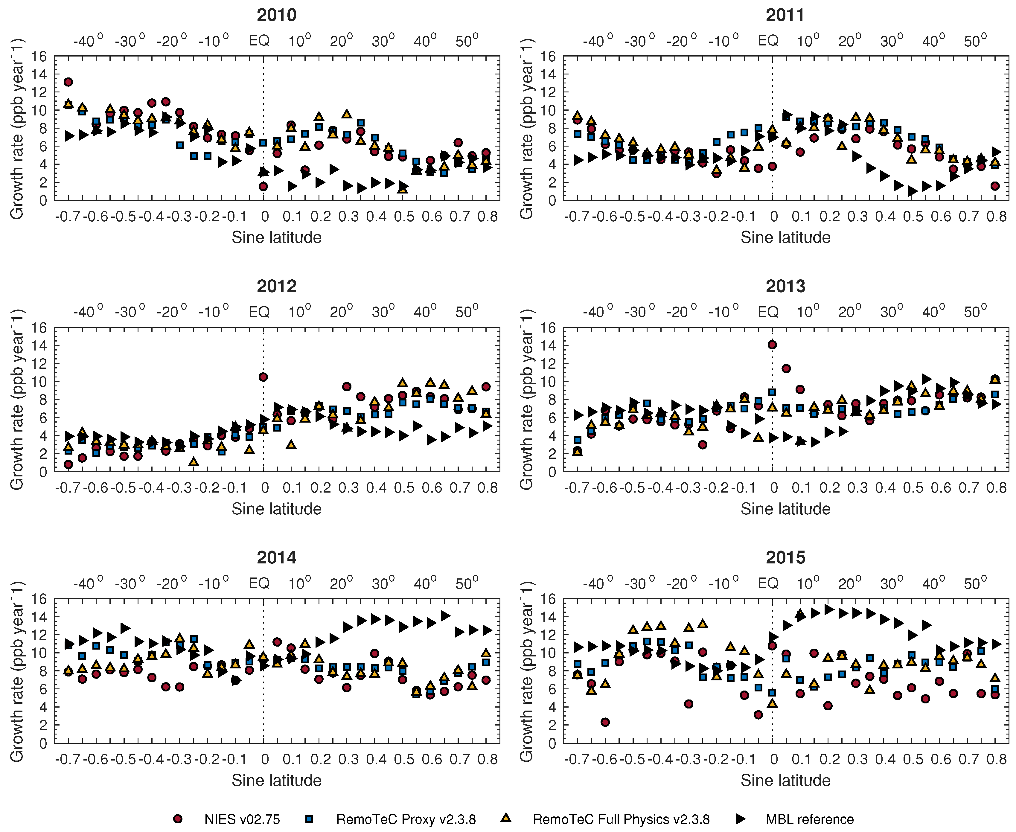
4.2. Evaluation at Latitude Bands
5. Summary and Conclusions
Author Contributions
Funding
Acknowledgments
Conflicts of Interest
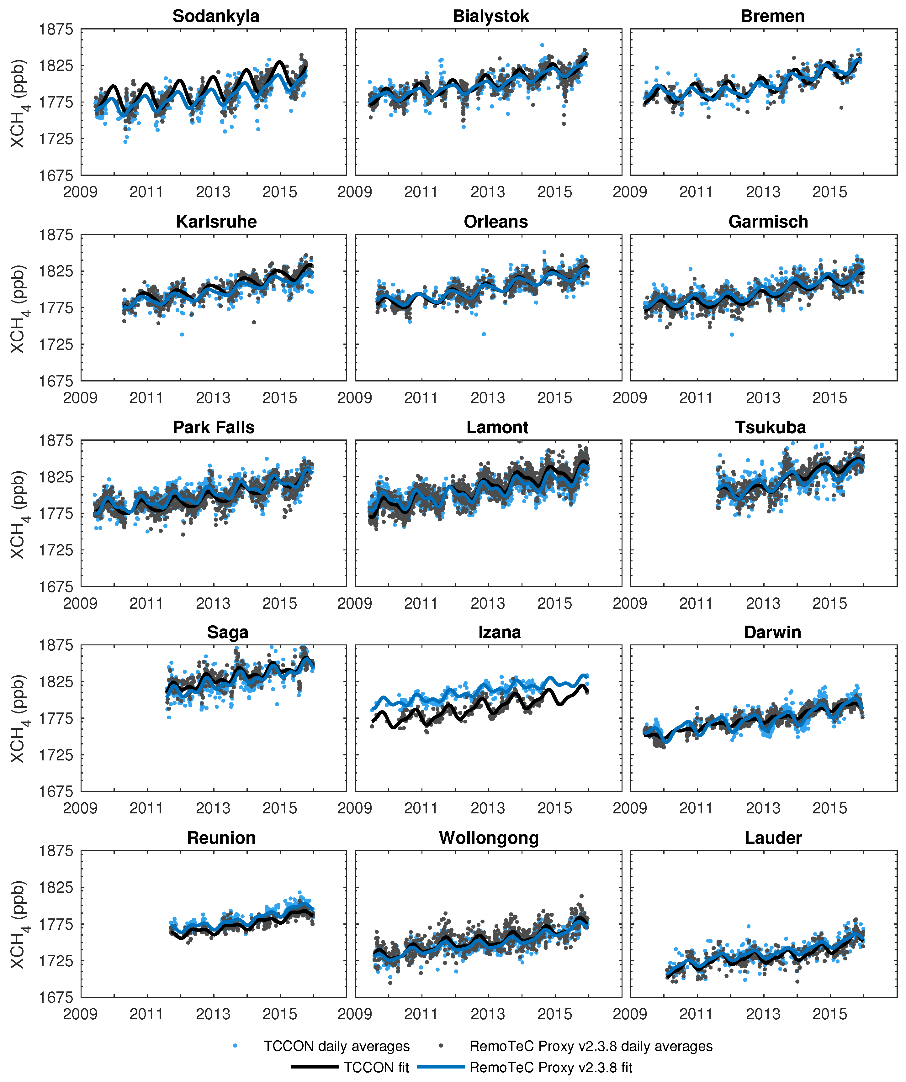
Appendix A. Daily Averages and Fitted Cycles
Appendix B. Computations for Dynamic Linear Model
Appendix C. Calculated Biases

| TCCON Site | NIES | RemoTeC Proxy | RemoTeC FP | |||
|---|---|---|---|---|---|---|
| Sodankylä | 8.49 | 14.33 | 16.00 | 16.75 | 13.17 | |
| Bialystok | 6.28 | 14.68 | 0.46 | 15.17 | 13.815 | 14.43 |
| Bremen | 7.37 | 13.25 | 0.52 | 14.80 | 14.54 | 14.26 |
| Karlsruhe | 2.29 | 13.59 | 14.04 | 10.15 | 13.21 | |
| Orléans | 5.53 | 13.44 | 0.85 | 13.21 | 14.51 | 13.48 |
| Garmisch | 7.23 | 14.94 | 2.41 | 14.21 | 15.53 | 15.01 |
| Park Falls | 5.71 | 14.26 | 3.41 | 14.77 | 13.67 | 13.98 |
| Lamont | 14.60 | 14.92 | 7.20 | 14.67 | ||
| Tsukuba | 6.69 | 14.42 | 15.36 | 17.47 | 16.23 | |
| Saga | 4.60 | 16.32 | 16.89 | 15.03 | 15.96 | |
| Izaña | 20.52 | 15.02 | 21.75 | 11.29 | 25.61 | 13.06 |
| Darwin | 8.36 | 0.05 | 10.51 | 8.21 | 10.28 | |
| Réunion | 3.56 | 8.20 | 6.96 | 9.47 | 16.15 | 10.31 |
| Wollongong | 13.43 | 11.90 | 1.93 | 13.69 | ||
| Lauder | 13.71 | 3.33 | 11.89 | 11.06 | 15.90 | |
| Mean | 4.06 | 13.50 | 1.50 | 13.63 | 13.44 | 13.84 |
Appendix D. Detailed Information about the Averaging Kernel Correction
| TCCON Site | NIES | RemoTeC FP | ||
|---|---|---|---|---|
| Diff. | std | Diff. | std | |
| Sodankylä | 5.45 | 1.67 | 13.26 | 2.25 |
| Bialystok | 3.66 | 1.38 | 11.90 | 3.30 |
| Bremen | 3.87 | 1.55 | 11.99 | 3.59 |
| Karlsruhe | 3.19 | 1.23 | 11.05 | 3.43 |
| Orléans | 3.11 | 1.30 | 10.93 | 3.38 |
| Garmisch | 3.10 | 1.27 | 11.15 | 3.77 |
| Park Falls | 2.43 | 0.92 | 8.74 | 3.06 |
| Lamont | 2.10 | 0.87 | 8.25 | 3.16 |
| Tsukuba | 2.82 | 1.00 | 11.41 | 3.89 |
| Saga | 2.62 | 1.19 | 12.01 | 3.39 |
| Izaña | 1.60 | 0.77 | 8.01 | 2.22 |
| Darwin | 1.19 | 0.32 | 9.39 | 0.71 |
| Réunion | 1.26 | 0.52 | 8.78 | 1.12 |
| Wollongong | 0.83 | 0.62 | 6.73 | 2.21 |
| Lauder | 1.52 | 0.68 | 7.10 | 2.04 |
| Mean | 2.58 | 1.02 | 10.05 | 2.77 |
References and Notes
- IPCC. Climate Change 2013: The Physical Science Basis. Contribution of Working Group I to the Fifth Assessment Report of the Intergovernmental Panel on Climate Change; Cambridge University Press: Cambridge, UK, 2013; p. 1535. [Google Scholar] [CrossRef]
- Butler, J.H.; Monzka, S.A. The NOAA Annual Greenhouse Gas Index (AGGI); NOAA Earth System Research Laboratory: Boulder, CO, USA, 2016.
- Saunois, M.; Bousquet, P.; Poulter, B.; Peregon, A.; Ciais, P.; Canadell, J.G.; Dlugokencky, E.J.; Etiope, G.; Bastviken, D.; Houweling, S.; et al. The global methane budget 2000–2012. Earth Syst. Sci. Data 2016, 8, 697–751. [Google Scholar] [CrossRef]
- Peters, C.N.; Bennartz, R.; Hornberger, G.M. Satellite-derived methane emissions from inundation in Bangladesh. J. Geophys. Res. Biogeosci. 2017, 122, 1137–1155. [Google Scholar] [CrossRef]
- Ganesan, A.L.; Rigby, M.; Lunt, M.F.; Parker, R.J.; Boesch, H.; Goulding, N.; Umezawa, T.; Zahn, A.; Chatterjee, A.; Prinn, R.G.; et al. Atmospheric observations show accurate reporting and little growth in India’s methane emissions. Nat. Commun. 2017, 8, 836. [Google Scholar] [CrossRef] [PubMed]
- Dlugokencky, E.J.; Masarie, K.A.; Tans, P.P.; Conway, T.J.; Xiong, X. Is the amplitude of the methane seasonal cycle changing? Atmos. Environ. 1997, 31, 21–26. [Google Scholar] [CrossRef]
- Khalil, M.A.K.; Shearer, M.J.; Rasmussen, R.A. Methane sinks, distribution and trends. In Atmospheric Methane: Its Role in the Global Environment; Khalil, M.A., Ed.; Springer: Portland, OR, USA, 1999; Chapter 6; pp. 86–97. [Google Scholar]
- Ko, M.K.W.; Newman, P.A.; Reimann, S.; Strahan, S.E. SPARC Report on Lifetimes of Stratospheric Ozone-Depleting Substances, Their Replacements, and Related Species; Technical Report; SPARC: Washington, DC, USA, 2013. [Google Scholar]
- Dlugokencky, E. NOAA/ESRL Trends in Atmospheric Methane. Available online: http://www.esrl.noaa.gov/gmd/ccgg/trends_ch4 (accessed on 12 December 2017).
- Saad, K.M.; Wunch, D.; Deutscher, N.M.; Griffith, D.W.T.; Hase, F.; De Mazière, M.; Notholt, J.; Pollard, D.F.; Roehl, C.M.; Schneider, M.; et al. Seasonal variability of stratospheric methane: Implications for constraining tropospheric methane budgets using total column observations. Atmos. Chem. Phys. 2016, 16, 14003–140024. [Google Scholar] [CrossRef]
- Aalto, T.; Hatakka, J.; Lallo, M. Tropospheric methane in northern Finland: Seasonal variations, transport patterns and correlations with other trace gases. Tellus B 2007, 59, 251–259. [Google Scholar] [CrossRef]
- Ostler, A.; Sussmann, R.; Rettinger, M.; Deutscher, N.M.; Dohe, S.; Hase, F.; Jones, N.; Palm, M.; Sinnhuber, B.M. Multistation intercomparison of column-averaged methane from NDACC and TCCON: Impact of dynamical variability. Atmos. Meas. Tech. 2014, 7, 4081–4101. [Google Scholar] [CrossRef]
- Tukiainen, S.; Railo, J.; Laine, M.; Hakkarainen, J.; Kivi, R.; Heikkinen, P.; Chen, H.; Tamminen, J. Retrieval of atmospheric CH4 profiles from Fourier transform infrared data using dimension reduction and MCMC. J. Geophys. Res. Atmos. 2016, 121, 10312–10327. [Google Scholar] [CrossRef]
- Yoshida, Y.; Kikuchi, N.; Morino, I.; Uchino, O.; Oshchepkov, S.; Bril, A.; Saeki, T.; Schutgens, N.; Toon, G.; Wunch, D.; et al. Improvement of the retrieval algorithm for GOSAT SWIR XCO2 and XCH4 and their validation using TCCON data. Atmos. Meas. Tech. 2013, 6, 1533–1547. [Google Scholar] [CrossRef]
- Schepers, D.; Guerlet, S.; Butz, A.; Landgraf, J.; Frankenberg, C.; Hasekamp, O.; Blavier, J.F.; Deutscher, N.M.; Griffith, D.W.T.; Hase, F.; et al. Methane retrievals from Greenhouse Gases Observing Satellite (GOSAT) shortwave infrared measurements: Performance comparison of proxy and physics retrieval algorithms. J. Geophys. Res. 2012, 117, D10307. [Google Scholar] [CrossRef]
- Buchwitz, M.; Reuter, M.; Schneising, O.; Boesch, H.; Guerlet, S.; Dils, B.; Aben, I.; Armante, R.; Bergamaschi, P.; Blumenstock, T.; et al. The Greenhouse Gas Climate Change Initiative (GHG-CCI): Comparison and quality assessment of near-surface-sensitive satellite-derived CO2 and CH4 global data sets. Remote Sens. Environ. 2015, 162, 344–362. [Google Scholar] [CrossRef]
- Dils, B.; Buchwitz, M.; Reuter, M.; Schneising, O.; Boesch, H.; Parker, R.; Guerlet, S.; Aben, I.; Blumenstock, T.; Burrows, J.P.; et al. The Greenhouse Gas Climate Change Initiative (GHG-CCI): Comparative validation of GHG-CCI SCIAMACHY/ENVISAT and TANSO-FTS/GOSAT CO2 and CH4 retrieval algorithm products with measurements from the TCCON. Atmos. Meas. Tech. 2014, 7, 1723–1744. [Google Scholar] [CrossRef]
- Parker, R.J.; Boesch, H.; McNorton, J.; Comyn-Platt, E.; Gloor, M.; Wilson, C.; Chipperfield, M.P.; Hayman, G.D.; Bloom, A.A. Evaluating year-to-year anomalies in tropical wetland methane emissions using satellite CH4 observations. Remote Sens. Environ. 2018, 211, 261–275. [Google Scholar] [CrossRef]
- Sheng, J.X.; Jacob, D.J.; Turner, A.J.; Maasakkers, J.D.; Benmergui, J.; Bloom, A.A.; Arndt, C.; Gautam, R.; Zavala-Araiza, D.; et al. 2010–2016 methane trends over Canada, the United States, and Mexico observed by the GOSAT satellite: Contributions from different source sectors. Atmos. Chem. Phys. 2018, 18, 12257–12267. [Google Scholar] [CrossRef]
- Laine, M.; Latva-Pukkila, N.; Kyrola, E. Analysing time-varying trends in stratospheric ozone time series using the state space approach. Atmos. Chem. Phys. 2014, 14, 9707–9725. [Google Scholar] [CrossRef]
- Yokota, T.; Yoshida, Y.; Eguchi, N.; Ota, Y.; Tanaka, T.; Watanabe, H.; Maksuytov, S. Global concentrations of CO2 and CH4 retrieved from GOSAT: First preliminary results. SOLA 2009, 5, 160–163. [Google Scholar] [CrossRef]
- Yoshida, Y.; Ota, Y.; Eguchi, N.; Kikuchi, N.; Nobuta, K.; Tran, H.; Morino, I.; Yokota, T. Retrieval algorithm for CO2 and CH4 column abundances from short-wavelength infrared spectral observations by the Greenhouse gases observing satellite. Atmos. Meas. Tech. 2011, 4, 717–734. [Google Scholar] [CrossRef]
- Butz, A.; Guerlet, S.; Hasekamp, O.; Schepers, D.; Galli, A.; Aben, I.; Frankenberg, C.; Hartmann, J.M.; Tran, H.; Kuze, A.; et al. Toward accurate CO2 and CH4 observations from GOSAT. Geophys. Res. Lett. 2011, 8, L14812. [Google Scholar] [CrossRef]
- Guerlet, S.; Butz, A.; Schepers, D.; Basu, S.; Hasekamp, O.P.; Kuze, A.; Yokota, T.; Blavier, J.F.; Deutscher, N.M.; Griffith, D.W.; et al. Impact of aerosol and thin cirrus on retrieving and validating XCO2 from GOSAT shortwave infrared measurements. J. Geophys. Res. Atmos. 2013, 118, 4887–4905. [Google Scholar] [CrossRef]
- Rodgers, D.C. Inverse Methods for Atmospheric Sounding—Theory and Practice; Series in Atmospheric, Oceanic and Planetary Physics; World Scientific: Singapore, 2000. [Google Scholar]
- Phillips, D. A technique for the numerical solution of certain integral equations of the first kind. J. Assoc. Comput. Mach. 1962, 9, 84–97. [Google Scholar] [CrossRef]
- Tikhonov, A. On the solution of incorrectly stated problems and a method of regularization. Dokl. Akad. Nauk SSSR 1963, 22, 501–504. [Google Scholar]
- Hasekamp, O.P.; Landgraf, J. Linearization of vector radiative transfer with respect to aerosol properties and its use in satellite remote sensing. J. Geophys. Res. 2005, 110, D04203. [Google Scholar] [CrossRef]
- Chevallier, F. On the parallelization of atmospheric inversions of CO2 surface fluxes within a variational framework. Geosci. Model Dev. 2013, 6, 783–790. [Google Scholar] [CrossRef]
- Wunch, D.; Toon, G.C.; Blavier, J.F.L.; Washenfelder, R.A.; Notholt, J.; Connor, B.J.; Griffith, D.W.T.; Sherlock, V.; Wennberg, P.O. The total carbon column observing network. Philos. Trans. R. Soc. A Math. Phys. Eng. Sci. 2011, 369, 2087–2112. [Google Scholar] [CrossRef]
- Karion, A.; Sweeney, C.; Tans, P.; Newberger, T. AirCore: An innovative atmospheric sampling system. J. Atmos. Ocean. Technol. 2010, 27, 1839–1853. [Google Scholar] [CrossRef]
- Wunch, D.; Toon, G.C.; Sherlock, V.; Deutscher, N.M.; Liu, X.; Feist, D.G.; Wennberg, P.O. The Total Carbon Column Observing Network’s GGG2014 Data Version; Oak Ridge National Laboratory: Oak Ridge, TN, USA, 2015. [CrossRef]
- Wunch, D.; Toon, G.C.; Wennberg, P.O.; Wofsy, S.C.; Stephens, B.B.; Fischer, M.L.; Uchino, O.; Abshire, J.B.; Bernath, P.; Biraud, S.C.; et al. Calibration of the total carbon column observing network using aircraft profile data. Atmos. Meas. Tech. 2010, 3, 1351–1362. [Google Scholar] [CrossRef]
- Sussmann, R.; Ostler, A.; Forster, F.; Rettinger, M.; Deutscher, N.M.; Griffith, D.W.T.; Hannigan, J.W.; Jones, N.; Patra, P.K. First intercalibration of column-averaged methane from the total carbon column observing network and the network for the detection of atmospheric composition change. Atmos. Meas. Tech. 2013, 6, 397–418. [Google Scholar] [CrossRef]
- Lindqvist, H.; O’Dell, C.W.; Basu, S.; Boesch, H.; Chevallier, F.; Deutscher, N.; Feng, L.; Fisher, B.; Hase, F.; Inoue, M.; et al. Does GOSAT capture the true seasonal cycle of carbon dioxide? Atmos. Chem. Phys. 2015, 15, 13023–13040. [Google Scholar] [CrossRef]
- Keppel-Aleks, G.; Wennberg, P.O.; Washenfelder, R.A.; Wunch, D.; Schneider, T.; Toon, G.C.; Andres, R.J.; Blavier, J.F.; Connor, B.; Davis, K.J.; et al. The imprint of surface fluxes and transport on variations in total column carbon dioxide. Biogeosciences 2012, 9, 875–891. [Google Scholar] [CrossRef]
- Wunch, D.; Wennberg, P.O.; Messerschmidt, J.; Parazoo, N.C.; Toon, G.C.; Deutscher, N.M.; Keppel-Aleks, G.; Roehl, C.M.; Randerson, J.T.; Warneke, T.; et al. The covariation of northern hemisphere summertime CO2 with surface temperature in boreal regions. Atmos. Chem. Phys. 2013, 13, 9447–9459. [Google Scholar] [CrossRef]
- Messerschmidt, J.; Chen, H.; Deutscher, N.M.; Gerbig, C.; Grupe, P.; Katrynski, K.; Koch, F.T.; Lavric, J.V.; Notholt, J.; Rodenbeck, C.; et al. Automated ground-based remote sensing measurements of greenhouse gases at the Bialystok site in comparison with collocated in situ measurements and model data. Atmos. Chem. Phys. 2012, 12, 6741–6755. [Google Scholar] [CrossRef]
- Deutscher, N.M.; Notholt, J.; Messerschmidt, J.; Weinzierl, C.; Warneke, T.; Petri, C.; Grupe, P.; Katrynski, K. TCCON Data from Bialystok (PL), Release GGG2014.R1. TCCON Data Archive, Hosted by CaltechDATA. 2015. [Google Scholar] [CrossRef]
- Notholt, J.; Petri, C.; Warneke, T.; Deutscher, N.; Buschmann, M.; Weinzierl, C.; Macatangay, R.; Grupe, P. TCCON Data from Bremen (DE), Release GGG2014.R0. TCCON Data Archive, Hosted by CaltechDATA. 2014. [Google Scholar] [CrossRef]
- Sussmann, R.; Rettinger, M. TCCON Data from Garmisch (DE), Release GGG2014.R2. TCCON Data Archive, Hosted by CaltechDATA. 2017. [Google Scholar] [CrossRef]
- Blumenstock, T.; Hase, F.; Schneider, F.M.; Garca, O.; Seplveda, E. TCCON Data from Izana (ES), Release GGG2014.R1. TCCON Data Archive, Hosted by CaltechDATA. 2017. [Google Scholar] [CrossRef]
- Hase, F.; Blumenstock, T.; Dohe, S.; Gross, J.; Kiel, M. TCCON Data from Karlsruhe (DE), Release GGG2014.R1. TCCON Data Archive, Hosted by CaltechDATA. 2017. [Google Scholar] [CrossRef]
- Wennberg, P.O.; Wunch, D.; Roehl, C.; Blavier, J.F.; Toon, G.C.; Allen, N.; Dowell, P.; Teske, K.; Martin, C.; Martin, J. TCCON Data from Lamont (US), Release GGG2014.R1. TCCON Data Archive, Hosted by CaltechDATA. 2017. [Google Scholar] [CrossRef]
- Warneke, T.; Messerschmidt, J.; Notholt, J.; Weinzierl, C.; Deutscher, N.; Petri, C.; Grupe, P.; Vuillemin, C.; Truong, F.; Schmidt, M.; et al. TCCON Data from Orléans (FR), Release GGG2014.R0. TCCON Data Archive, Hosted by CaltechDATA. 2017. [Google Scholar] [CrossRef]
- Washenfelder, R.A.; Toon, G.C.; Blavier, J.F.L.; Yang, Z.; Allen, N.T.; Wennberg, P.O.; Vay, S.A.; Matross, D.M.; Daube, B.C. Carbon dioxide column abundances at the Wisconsin Tall Tower site. J. Geophys. Res. 2006, 111, 1–11. [Google Scholar] [CrossRef]
- Wennberg, P.O.; Roehl, C.; Wunch, D.; Toon, G.C.; Blavier, J.F.; Washenfelder, R.; Keppel-Aleks, G.; Allen, N.; Ayers, J. TCCON Data from Park Falls (US), Release GGG2014.R1. TCCON Data Archive, Hosted by CaltechDATA. 2017. [Google Scholar] [CrossRef]
- Kawakami, S.; Ohyama, H.; Arai, K.; Okumura, H.; Taura, C.; Fukamachi, T.; Sakashita, M. TCCON Data from Saga (JP), Release GGG2014.R0. TCCON Data Archive, Hosted by CaltechDATA. 2017. [Google Scholar] [CrossRef]
- Ohyama, H.; Morino, I.; Nagahama, T.; Machida, T.; Suto, H.; Oguma, H.; Sawa, Y.; Matsueda, H.; Sugimoto, N.; Nakane, H.; et al. Column-averaged volume mixing ratio of CO2 measured with ground-based Fourier transform spectrometer at Tsukuba. J. Geophys. Res. 2009, 114, D18303. [Google Scholar] [CrossRef]
- Morino, I.; Matsuzaki, T.; Horikaw, M. TCCON Data from Tsukuba (JP), 125HR, Release GGG2014.R2. TCCON Data Archive, Hosted by CaltechDATA. 2017. [Google Scholar] [CrossRef]
- Kivi, R.; Heikkinen, P.; Kyrö, E. TCCON Data from Sodankylä (FI), Release GGG2014.R0. TCCON Data Archive, Hosted by CaltechDATA. 2017. [Google Scholar] [CrossRef]
- Kivi, R.; Heikkinen, P. Fourier transform spectrometer measurements of column CO2 at Sodankylä, Finland. Geosci. Instrum. Method Data Syst. 2016, 5, 271–279. [Google Scholar] [CrossRef]
- Deutscher, N.M.; Griffith, D.W.T.; Bryant, G.W.; Wennberg, P.O.; Toon, G.C.; Washenfelder, R.A.; Keppel-Aleks, G.; Wunch, D.; Yavin, Y.G.; Allen, N.T.; et al. Total column CO2 measurements at Darwin, Australia—Site description and calibration against in situ aircraft profiles. Atmos. Meas. Tech. 2010, 3, 947–958. [Google Scholar] [CrossRef]
- Griffith, D.W.T.; Deutscher, N.; Velazco, V.A.; Wennberg, P.O.; Yavin, Y.; Keppel Aleks, G.; Washenfelder, R.; Toon, G.C.; Blavier, J.F.; Paton-Walsh, C.; et al. TCCON Data from Darwin (AU), Release GGG2014.R0. TCCON Data Archive, Hosted by CaltechDATA. 2014. [Google Scholar] [CrossRef]
- Sherlock, V.; Connor, B.; Robinson, J.; Shiona, H.; Smale, D.; Pollard, D.F. TCCON Data from Lauder (NZ), 125HR, Release GGG2014.R0. TCCON Data Archive, Hosted by CaltechDATA. 2014. [Google Scholar] [CrossRef]
- Pollard, D.F.; Sherlock, V.; Robinson, J.; Deutscher, N.M.; Connor, B.; Shiona, H. The total carbon column observing network site description for Lauder, New Zealand. Earth Syst. Sci. Data 2017, 9, 977–992. [Google Scholar] [CrossRef]
- De Mazière, M.; Sha, M.K.; Desmet, F.; Hermans, C.; Scolas, F.; Kumps, N.; Metzger, J.M.; Duflot, V.; Cammas, J.P. TCCON Data from Réunion Island (RE), Release GGG2014.R1. TCCON Data Archive, Hosted by CaltechDATA. 2017. [Google Scholar] [CrossRef]
- Griffith, D.W.T.; Velazco, V.A.; Deutscher, N.; Paton-Walsh, C.; Jones, N.; Wilson, S.; Macatangay, R.C.; Kettlewell, G.; Buchholz, R.R.; Riggenbach, M. TCCON Data from Wollongong (AU), Release GGG2014.R0. TCCON Data Archive, Hosted by CaltechDATA. 2017. [Google Scholar] [CrossRef]
- Dlugokencky, E.; Lang, P.; Crotwell, A.; Masarie, K.; Crotwell, M. Atmospheric Methane Dry Air Mole Fractions from the NOAA ESRL Carbon Cycle Cooperative Global Air Sampling Network. Available online: ftp://aftp.cmdl.noaa.gov/data/trace_gases/ch4/flask/surface/ (accessed on 3 August 2017).
- Thoning, K.W.; Tans, P.P.; Komhyr, W.D. Atmospheric carbon dioxide at Mauna Loa Observatory: 2. Analysis of the NOAA GMCC data, 1974–1985. J. Geophys. Res. 1989, 94, 8549–8565. [Google Scholar] [CrossRef]
- Tsuruta, A.; Aalto, T.; Backman, L.; Hakkarainen, J.; van der Laan-Luijkx, I.T.; Krol, M.C.; Spahni, R.; Houweling, S.; Laine, M.; Dlugokencky, E.; et al. Global methane emission estimates for 2000–2012 from CarbonTracker Europe-CH4 v1.0. Geosci. Model Dev. 2017, 10, 1261–1289. [Google Scholar] [CrossRef]
- Peters, W.; Miller, J.B.; Whitaker, J.; Denning, A.S.; Hirsch, A.; Krol, M.C.; Zupanski, D.; Bruhwiler, L.; Tans, P.P. An ensemble data assimilation system to estimate CO2 surface fluxes from atmospheric trace gas observations. J. Geophys. Res. 2005, 110, D24304. [Google Scholar] [CrossRef]
- Krol, M.; Houweling, S.; Bregman, B.; van den Broek, M.; Segers, A.; van Velthoven, P.; Peters, W.; Dentener, F.; Bergamaschi, P. The two-way nested global chemistry-transport zoom model TM5: Algorithm and applications. Atmos. Chem. Phys. 2005, 5, 417–432. [Google Scholar] [CrossRef]
- Zhou, M.; Dils, B.; Wang, P.; Detmers, R.; Yoshida, Y.; O’Dell, C.W.; Feist, D.G.; Velazco, V.A.; Schneider, M.; De Mazière, M. Validation of TANSO-FTS/GOSAT XCO2 and XCH4 glint mode retrievals using TCCON data from near-ocean sites. Atmos. Meas. Tech. 2016, 9, 1415–1430. [Google Scholar] [CrossRef]
- Dee, D.P.; Uppala, S.M.; Simmons, A.J.; Berrisford, P.; Poli, P.; Kobayashi, S.; Andrae, U.; Balmaseda, M.A.; Balsamo, G.; Bauer, P.; et al. The ERA-Interim reanalysis: Configuration and performance of the data assimilation system. Q. J. R. Meteorol. Soc. 2011, 137, 553–597. [Google Scholar] [CrossRef]
- Rodgers, C.D.; Connor, B.J. Intercomparison of remote sounding instruments. J. Geophys. Res. 2003, 108, 4116. [Google Scholar] [CrossRef]
- Reuter, M.; Bovensmann, H.; Buchwitz, M.; Burrows, J.; Connor, B.J.; Deutscher, N.M.; Griffith, D.W.T.; Heymann, J.K.A.G.; Messerschmidt, J.; Notholt, J.; et al. Retrieval of atmospheric CO2 with enhanced accuracy and precision from SCIAMACHY: Validation with FTS measurements and comparison with model results. J. Geophys. Res. 2011, D04301. [Google Scholar] [CrossRef]
- Wunch, D.; Wennberg, P.O.; Toon, G.C.; Connor, B.J.; Fisher, B.; Osterman, G.B.; Frankenberg, C.; Mandrake, L.; O’Dell, C.; Ahonen, P.; et al. A method for evaluating bias in global measurements of CO2 total columns from spac. Atmos. Chem. Phys. 2011, 11, 12317–12337. [Google Scholar] [CrossRef]
- Schneising, O.; Bergamaschi, P.; Bovensmann, H.; Buchwitz, M.; Burrows, J.P.; Deutscher, N.M.; Griffith, D.W.T.; Heymann, J.; Macatangay, R.; Messerschmidt, J.; et al. Atmospheric greenhouse gases retrieved from SCIAMACHY: Comparison to ground-based FTS measurements and model results. Atmos. Chem. Phys. 2012, 12, 1527–1540. [Google Scholar] [CrossRef]
- Ball, W.T.; Alsing, J.; Mortlock, D.J.; Rozanov, E.V.; Tummon, F.; Haigh, J.D. Reconciling differences in stratospheric ozone composites. Atmos. Chem. Phys. 2017, 17, 12269–12302. [Google Scholar] [CrossRef]
- Roininen, L.; Laine, M.; Ulich, T. Time-varying ionosonde trend: Case study of Sodankylä hmF2 data 1957–2014. J. Geophys. Res. Space Phys. 2015, 120, 6851–6859. [Google Scholar] [CrossRef]
- Dlugokencky, E.J.; Steele, L.P.; Lang, P.M.; Masarie, K.A. The growth rate and distribution of atmospheric methane. J. Geophys. Res. 1994, 99, 17021–17043. [Google Scholar] [CrossRef]
- Ishizawa, M.; Uchino, O.; Morino, I.; Inoue, M.; Yoshida, Y.; Mabuchi, K.; Shirai, T.; Tohjima, Y.; Maksyutov, S.; Ohyama, H.; et al. Large XCH4 anomaly in summer 2013 over northeast Asia observed by GOSAT. Atmos. Chem. Phys. 2016, 16, 9149–9161. [Google Scholar] [CrossRef]
- Detmers, R. System Verification Report (SVR) GHG-CCI Phase 2 CRDP#3 for Sub-System CH4_GOS_SRPR version 3. Available online: http://www.esa-ghg-cci.org/?q=webfm_send/364 (accessed on 30 January 2018).
- Detmers, R. System Verification Report (SVR) GHG-CCI Phase 2 CRDP#3 for Sub-System CH4_GOS_SRFP Version 3. Available online: http://www.esa-ghg-cci.org/?q=webfm_send/365 (accessed on 30 January 2018).
- Reuter, M.; Bösch, H.; Bovensmann, H.; Bril, A.; Buchwitz, M.; Butz, A.; Burrows, J.P.; O’Dell, C.W.; Guerlet, S.; Hasekamp, O.; et al. A joint effort to deliver satellite retrieved atmospheric CO2 concentrations for surface flux inversions: The ensemble median algorithm EMMA. Atmos. Chem. Phys. 2013, 13, 1771–1780. [Google Scholar] [CrossRef]
- Petris, G.; Petrone, S.; Campagnoli, P. Dynamic Linear Models with R, Use R! Springer: Berlin, Germany, 2009. [Google Scholar]
- Durbin, T.; Koopman, S. Time Series Analysis by State Space Methods, 2nd ed.; Oxford Statistical Science Series; Oxford University Press: Oxford, UK, 2013. [Google Scholar] [CrossRef]


© 2019 by the authors. Licensee MDPI, Basel, Switzerland. This article is an open access article distributed under the terms and conditions of the Creative Commons Attribution (CC BY) license (http://creativecommons.org/licenses/by/4.0/).
Share and Cite
Kivimäki, E.; Lindqvist, H.; Hakkarainen, J.; Laine, M.; Sussmann, R.; Tsuruta, A.; Detmers, R.; Deutscher, N.M.; Dlugokencky, E.J.; Hase, F.; et al. Evaluation and Analysis of the Seasonal Cycle and Variability of the Trend from GOSAT Methane Retrievals. Remote Sens. 2019, 11, 882. https://doi.org/10.3390/rs11070882
Kivimäki E, Lindqvist H, Hakkarainen J, Laine M, Sussmann R, Tsuruta A, Detmers R, Deutscher NM, Dlugokencky EJ, Hase F, et al. Evaluation and Analysis of the Seasonal Cycle and Variability of the Trend from GOSAT Methane Retrievals. Remote Sensing. 2019; 11(7):882. https://doi.org/10.3390/rs11070882
Chicago/Turabian StyleKivimäki, Ella, Hannakaisa Lindqvist, Janne Hakkarainen, Marko Laine, Ralf Sussmann, Aki Tsuruta, Rob Detmers, Nicholas M. Deutscher, Edward J. Dlugokencky, Frank Hase, and et al. 2019. "Evaluation and Analysis of the Seasonal Cycle and Variability of the Trend from GOSAT Methane Retrievals" Remote Sensing 11, no. 7: 882. https://doi.org/10.3390/rs11070882
APA StyleKivimäki, E., Lindqvist, H., Hakkarainen, J., Laine, M., Sussmann, R., Tsuruta, A., Detmers, R., Deutscher, N. M., Dlugokencky, E. J., Hase, F., Hasekamp, O., Kivi, R., Morino, I., Notholt, J., Pollard, D. F., Roehl, C., Schneider, M., Sha, M. K., Velazco, V. A., ... Tamminen, J. (2019). Evaluation and Analysis of the Seasonal Cycle and Variability of the Trend from GOSAT Methane Retrievals. Remote Sensing, 11(7), 882. https://doi.org/10.3390/rs11070882