1. Introduction
Airborne LiDAR (Light Detection and Ranging) has been beneficial in the field of forestry for several years because of its ability to produce very accurate information about terrain [
1,
2]. Among the information obtained from LiDAR data, vegetation height is an important variable for forest management. Furthermore, metrics related to height are key explanatory variables for many attributes such as volume [
3,
4,
5] or biomass [
6,
7]. The height is therefore used extensively, despite the fact that it is well known for underestimation [
8,
9].
Several measurable factors have been proposed to explain underestimations, including: (i) pulse density, (ii) pattern of scan (sensors), (iii) scan angles, (iv) contract specific parameters (flying altitude, pulse repetition frequency), (v) territory characteristics (stand density and species) and (vi) ground overestimation [
10,
11,
12,
13,
14,
15,
16,
17,
18,
19,
20,
21,
22,
23,
24,
25,
26,
27,
28].
Lefsky et al. [
25] determined that pulse density is the principal parameter determining tree height underestimation. According to several other studies, pulse density has an impact on underestimations of height, depending on the scale of the study and on the mean pulse density of the LiDAR survey. Bater et al. [
24] analyzed, at plot scale, the impact of different pulse densities at the maximum height, and concluded that maximum height was significantly different between pulse densities varying within 2% to 4%. Treitz et al. [
23] also studied the impact of pulse density (3.2 pulses/m
2 decimated to 0.5 pulses/m
2) on several forest inventory variables such as tree top height, but concluded that at plot scale, the pulse density had no significant effect on tree top height. Furthermore, at a tree scale, Sibona et al. [
17] concluded that heights obtained by LiDAR were not significantly different to those measured in the field for pulse densities higher than 5 pulses/m
2. Moreover, Yu et al. [
27] demonstrated that height underestimation increased as the pulse density decreased and that the underestimation between 2.5 and 5 pulses/m
2 was greater than between 5 and 10 pulses/m
2. Additionally, Naesset & Okland [
26] stated that the most efficient way to increase the height precision is by increasing the pulse density. Finally, Roussel et al. [
10] demonstrated that at a 4 m
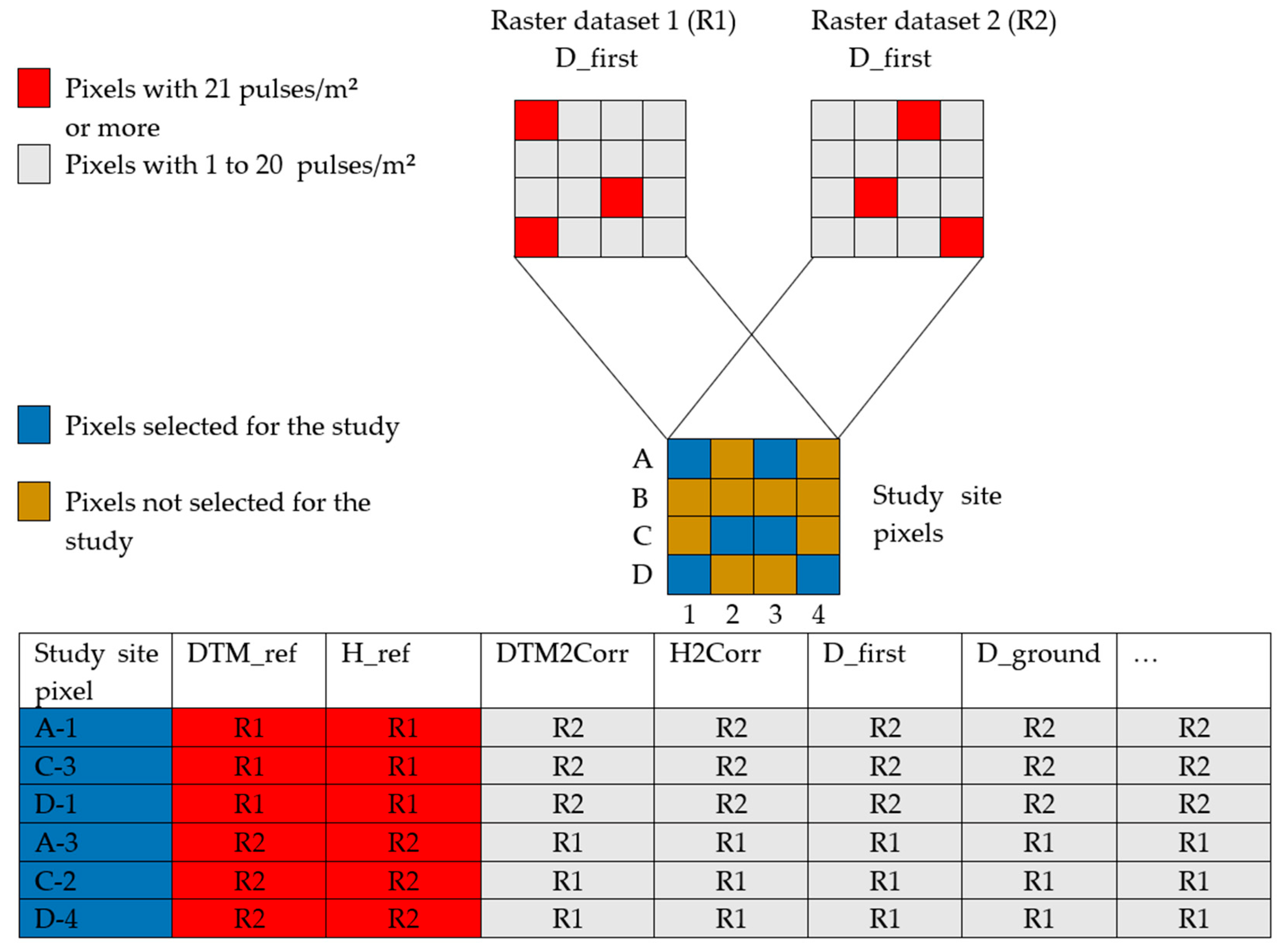
2 scale, for a pulse density of 21 pulses/m
2 or higher, underestimation would be smaller than 0.10 m. The authors also analyzed the scale effect and concluded that for the same density, the scale also significantly impacted the underestimation [
10].
Other parameters may also influence the underestimation of the height. First, the scan pattern used influences the distribution of pulses and therefore the pulses/m
2. Optech and Leica sensors use oscillating mirrors, while Riegl uses a rotating polygon. The first category produces zigzag scan lines (heterogeneous distribution of pulses), while the second uses parallel scan lines (homogeneous distribution of pulses) [
11]. Second, scan angles influence the estimation of forest height. The effect of this factor is different, depending on the forest structure [
12]. For example, Holmgren et al. [
13] simulated four different forest types to evaluate the underestimation caused by scan angles. Their results show that long crown species like spruce are more affected than short crown species like pine. Furthermore, dense stands are less affected than sparser stands. Montaghi [
14] compared scan angles at nadir with scan angles between 0 to 20 degrees, and concluded that scan angles smaller than 20 degrees have no significant impact on stand measured height. Third, higher flying altitudes or increased pulse frequencies reduce the pulse intensity, and thus, require larger and denser backscatter areas to return the pulse to the sensor. Ultimately, lower pulse intensities increase the pulse penetration into foliage, and thereby, underestimate height [
15]. Hopkinson [
15] varied pulse intensities between surveys for 24 plots and demonstrated that decreasing pulse intensity lead to an increase in foliage penetration varying from 0.15 to 0.61 m with other parameters remaining constant. Fourth, height underestimation is also influenced by crown shape [
16], stand density and species composition [
8,
17,
18]. Sibona et al. [
17] showed between three species that European larch had the smallest mean absolute difference (0.95 m) compared to scots pine and European spruce, which had respective underestimations of 1.4 m and 1.13 m. Furthermore, Yu et al. [
27] demonstrated that underestimation varied according to species. In order, pine is the most affected, followed by spruce and birch. Finally, height underestimation is also influenced by an overestimation of the digital terrain model (DTM). Hyyppä et al. [
28] demonstrated that DTM error varies according to slopes, undergrowth vegetation and forest cover type. Indeed, slopes can lead to overestimations, in part due to beam divergence. Beam divergence has a greater effect on steep slopes than on flat ground. This divergence causes horizontal errors, and consequently, on steep slopes, vertical errors [
19,
28]. Tinkham et al. [
19], for example, demonstrated that a slope greater than 30 degrees has a significant vertical DTM error and that vegetation structure has no significant impact on the DTM values. Also, Hyyppä et al. [
28] demonstrated that DTM accuracy gradually decreases as the slope increases. Furthermore, the authors show that resulting DTM error in forested areas is greater than in open areas. Finally, dense stands [
20] and understory vegetation [
21] increase DTM overestimations.
In conclusion, factors influencing the precision of altitude values from airborne LiDAR depend on two main elements: (i) the capability of the pulse to reach the ground [
19,
22], and (ii) its probability to hit the canopy. Both phenomena are analyzed in this work in order to evaluate their quantitative impacts and to calculate models to correct the resulting difference between the reference value and the value to correct (here and after called bias).
The goal of this study is first to propose an adjustment model to correct the DTM bias, and ultimately, to propose an adjustment model to correct canopy height model (CHM) bias for a wide range of site and acquisition conditions. Although several factors have been evaluated separately, no study has accurately measured these factors and proposed adjustments on DTM and CHM in a variety of forest conditions.
3. Modeling
Modeling the adjustments for DTM and CHM values consisted of three methodological steps that involved developing first a linear mixed model, followed by a non-linear model, and finally a non-linear mixed model. These steps were done for both DTM and CHM adjustment models with SAS (version 9.4, SAS Institute Inc., Cary, NC, USA).
3.1. Linear Mixed Model
For DTM and CHM adjustments, linear mixed regressions were performed to determine the independent variables contributing to the models. The independent variables tested were H2Corr (
Table 1), LiDAR variables shown in
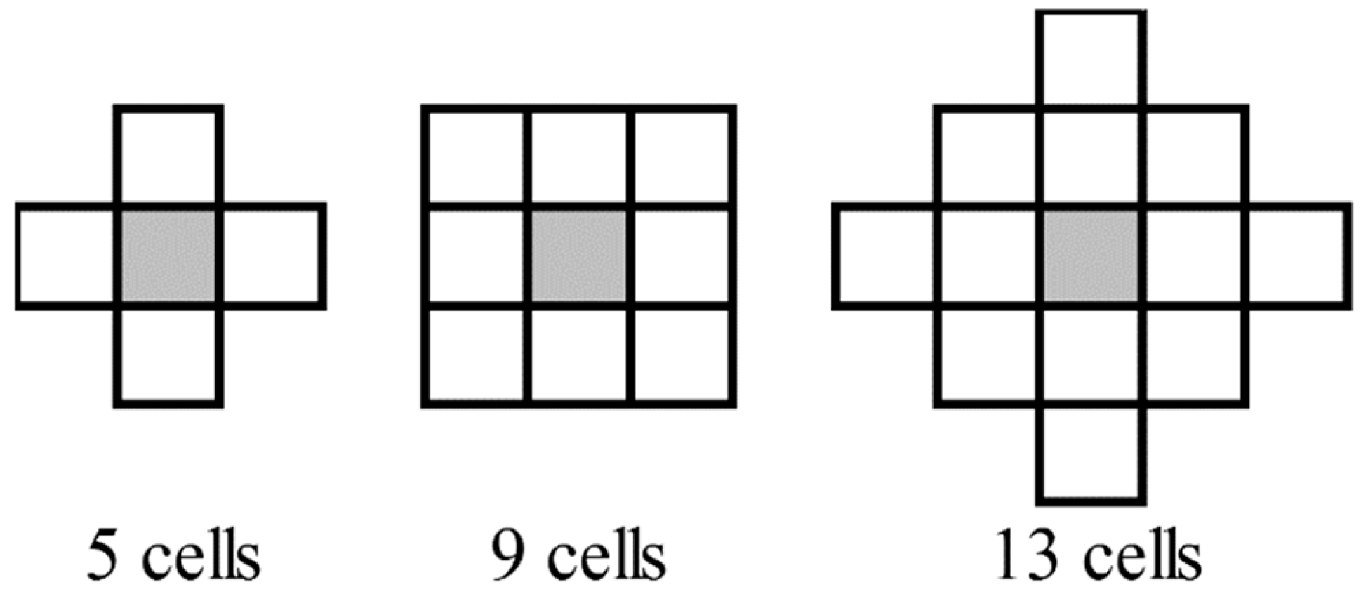
Table 3, the sensor and the study sites. At this point, continuous variables were converted into classes to find the form of the relationship that reflects the effect of the variables. The variables D_first and D_ground were already in a class format as integer numbers. The number of classes per variable were respectively of 13, 8, 8, 8, 3, 9 for H2Corr, H_STD5, H_STD9, H_STD13, scan angles and slopes. We constructed models having a maximum of three independent variables including all interactions between them. At the beginning, a limit of three independent variables was imposed in order to have an easy to use model. To verify that more variables were not needed, residuals of the other variables were tested in each model. If residuals had revealed that more variables were needed, the maximum number of variables would have been adjusted.
Random effects among the 26 sites were estimated by testing the intercept coefficient using conditional and marginal predictions. First, conditional predictions were tested, taking into account the random effects of the study sites, and second, marginal predictions were tested by omitting these effects. For each linear mixed model, residuals were tested against all LiDAR acquisition variables to evaluate if variables that were not included in the fixed effects were explaining the residual variation.
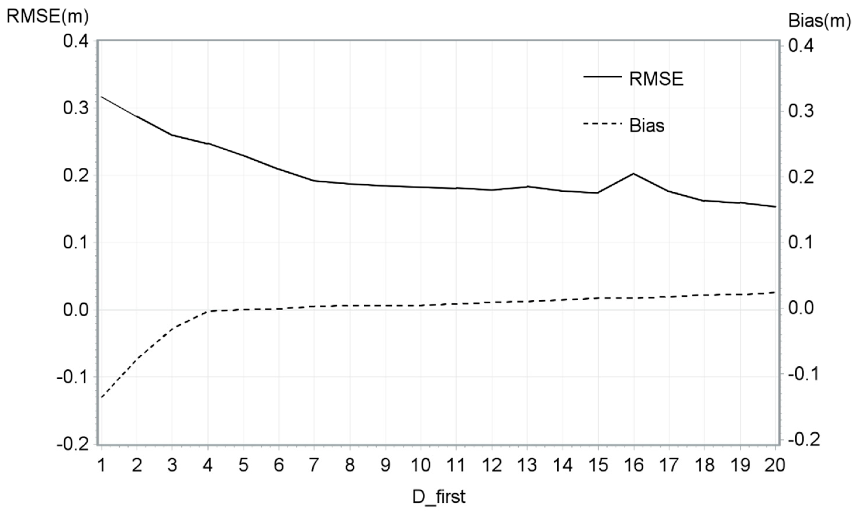
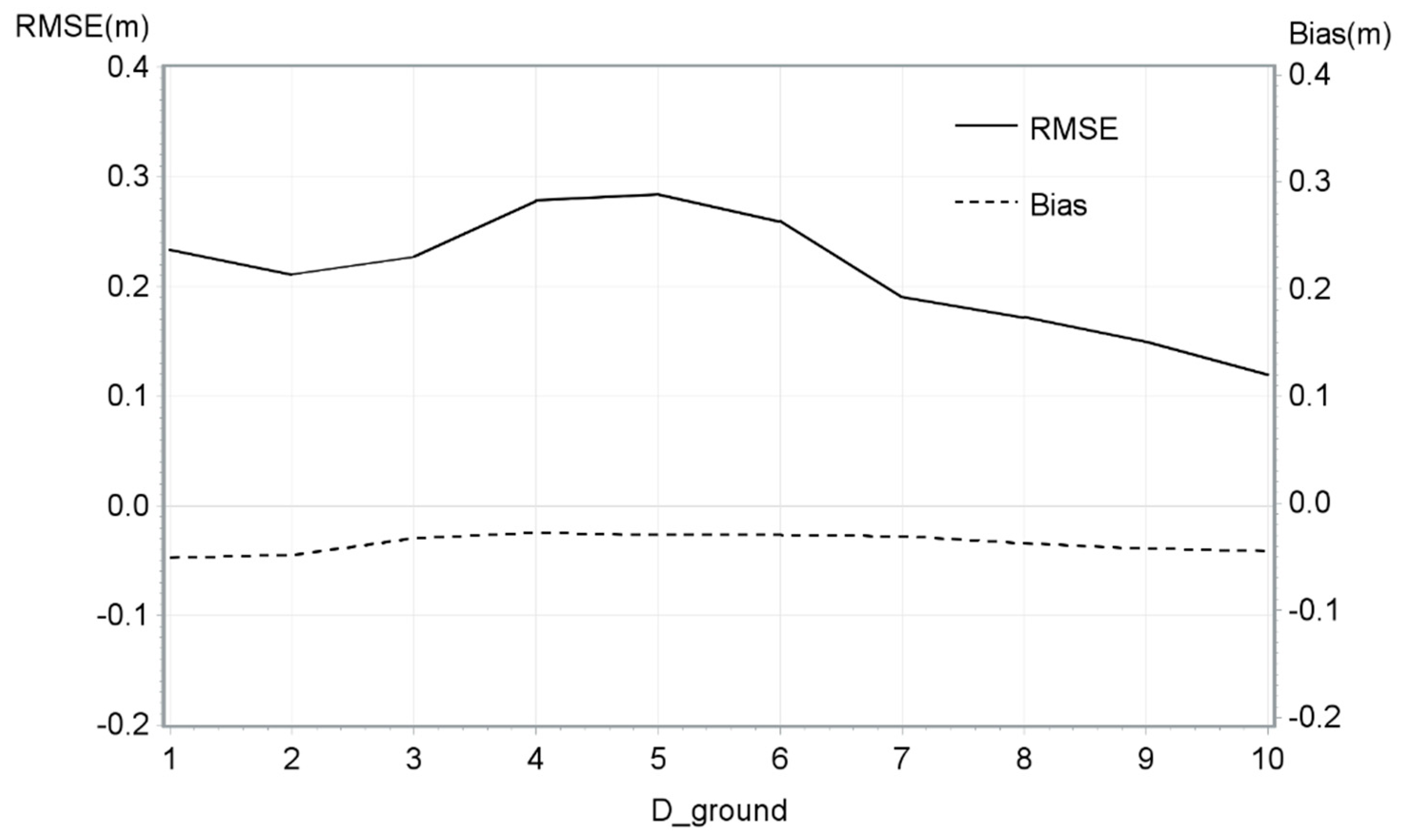
Models tested the influence of D_first, D_ground, H2Corr and H_STD for the three neighborhood scales (H_STD5, H_STD9 and H_STD13). For the DTM adjustment models, there were no significant variables. The residuals were tested for sensors, terrain slopes, and scan angles. As a result, the methodology stopped here for the DTM and no specific adjustments were made.
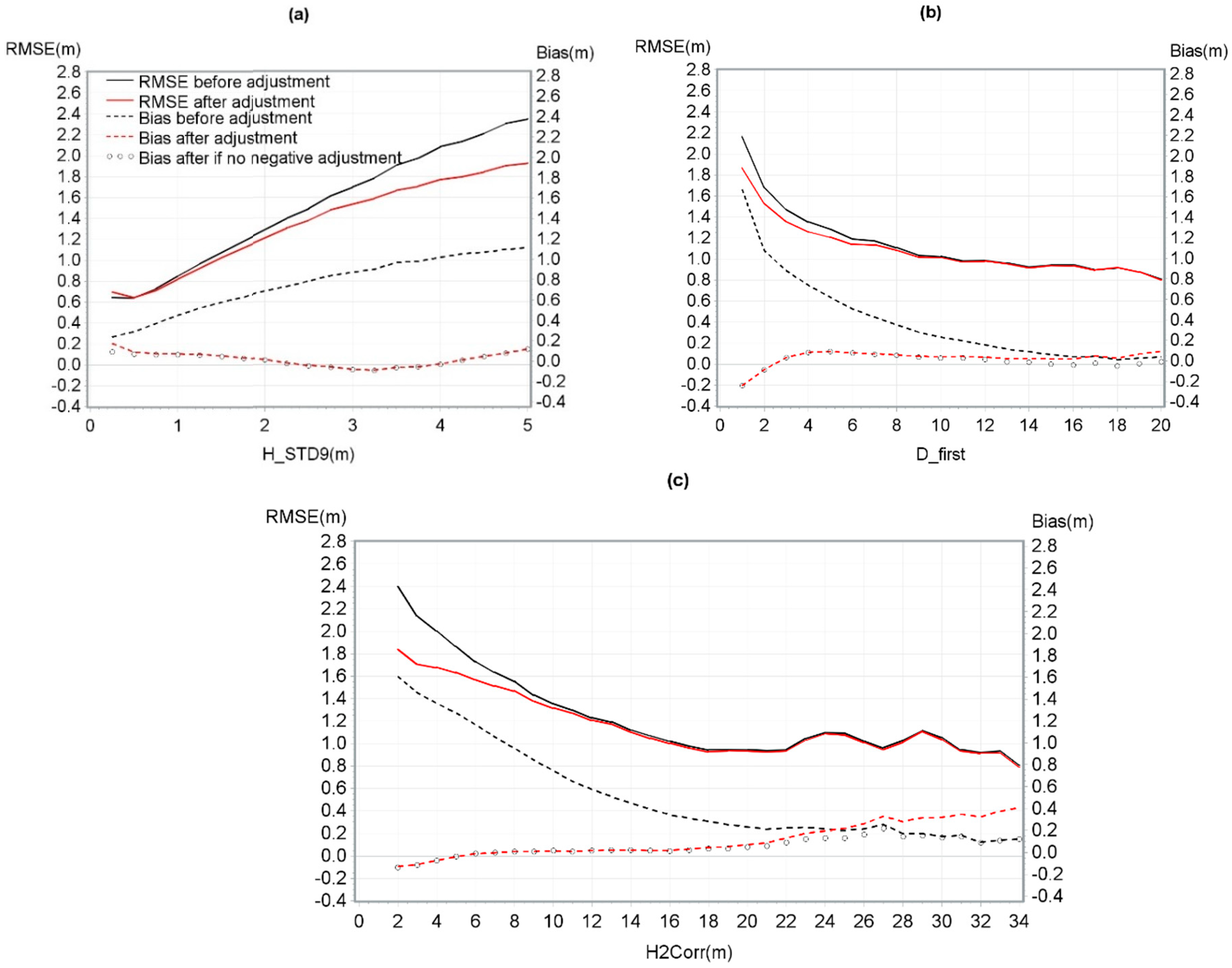
For the canopy height adjustment models, the significant variables which were selected were H2Corr, D_first and H_STD9. An analysis of the residuals of these three independent variables indicated that it was appropriate to remove the pixels with terrain slopes greater than 45 degrees from the other analyses. Above these slope angles, the distribution of residuals showed a pattern indicating that this effect should be considered by the model. Even though the three neighbourhood scales for the height standard deviation were significant, the nine-cell neighbourhood was selected among the three based on R2 values. Moreover, marginal prediction was selected because the R2 barely increased when the study site was considered (mean difference of 1%). We concluded that in the case of this database, the study site (contractor, sensor, flight altitude and pulse frequency) did not influence height adjustment. Also, this led to a general model applicable to all the conditions tested in this study.
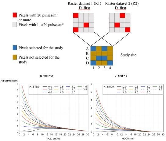
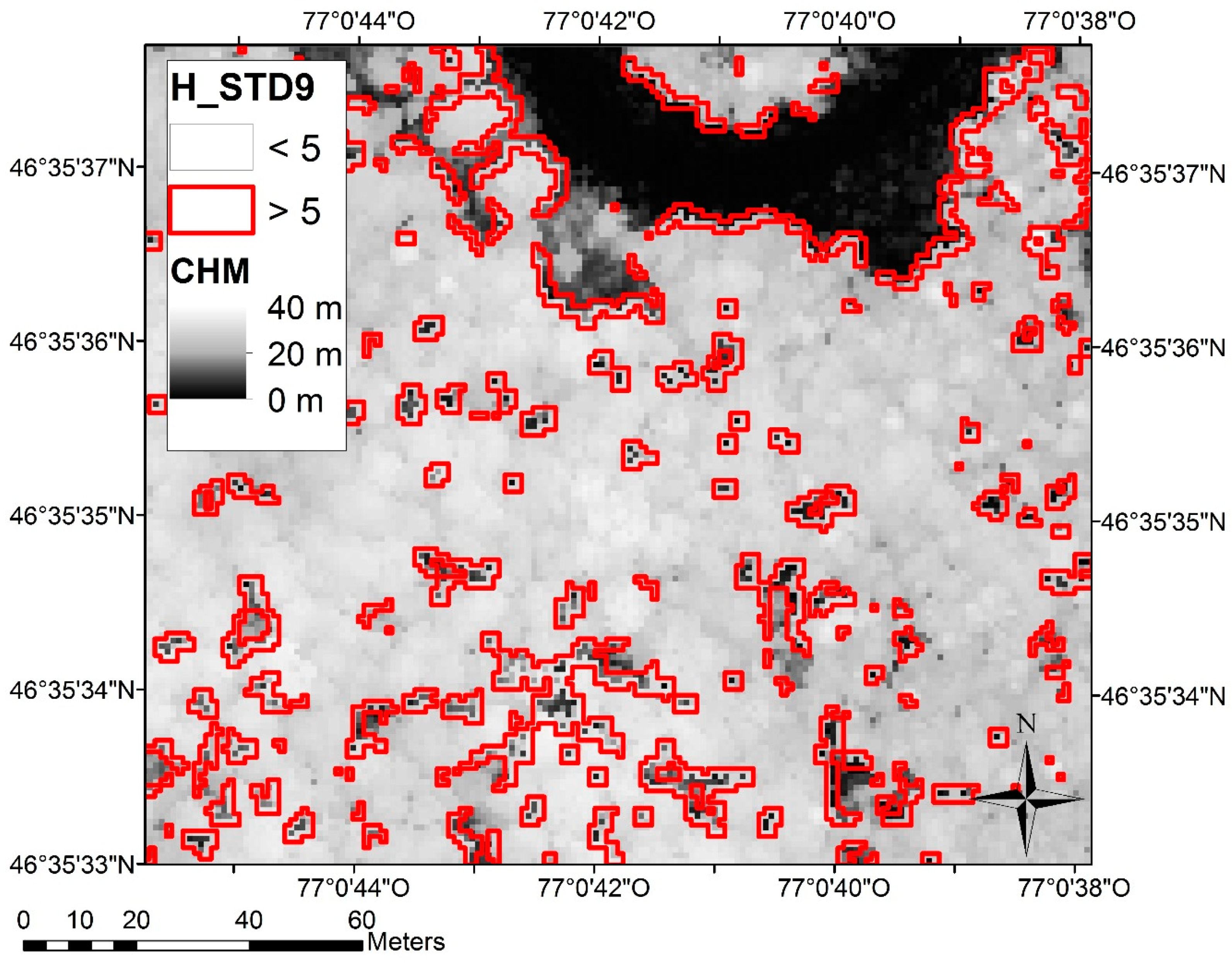
Based on visual observation, H_STD9 greater than five were recoded to five. This manipulation was applied because theses pixels represented forest canopy opening extremity (
Figure 4). In these pixels, height was very variable depending on where pulses fell. As the adjustment increased with STD, unrealistic adjustments were predicted in these areas (8% of the pixels). A final linear mixed model was performed and an adjustment average was calculated for each combination of variable class (2080 combinations resulting from 20 D_first, 8 H_STD9 and 13 H2Corr classes). These averages were the inputs for the non-linear model.
3.2. Non-Linear Model
A non-linear model was used to find the shape of the equation. This model was weighted with the number of observations by class in order to give a more important weight for the more frequent values.
First, to visualize the equation form, one model was made for each H_STD9 and H2Corr class according to D_first. Thereby, the equation of the global form of the adjustments was simplified in the following way:
where α, β and ω were the model parameters.
Second, the estimates of parameter β were visualized for each H2Corr class according to H_STD9. It was concluded that it was best represented by a linear equation:
Thereafter, estimates of β0 and β1 were visualized according to H2Corr. They respectively followed a simplification of the differential form of the Chapman-Richards equation and of an exponential curve.
Finally, the visualization of the two other parameters (ω and α) for each H2Corr classes according to H_STD9 simplified the selection of parameters during the modeling process.
Consequently, the non-linear model final equation was:
where:
where ε
jm was the error term of the jth pixel and for the mth study site.
3.3. Non-Linear Mixed Model
The final non-linear model equation was used in a non-linear mixed model to find the fixed coefficients with SAS® NLMIXED procedure. The random coefficient (δm) was added on the vertical intercept (α). The database included 3,263,872 pixels. For this model, 50% of the pixels from the original database of each site were randomly selected and used for the calibration.
3.4. Validation
The other 50% of the pixels were used for the validation. The CHM adjustment model was validated using this validation dataset. Thus, the model was applied on H2Corr and was compared with H_ref. The R2, the remaining bias on the corrected LiDAR height and the RMSE were then calculated.
6. Conclusions
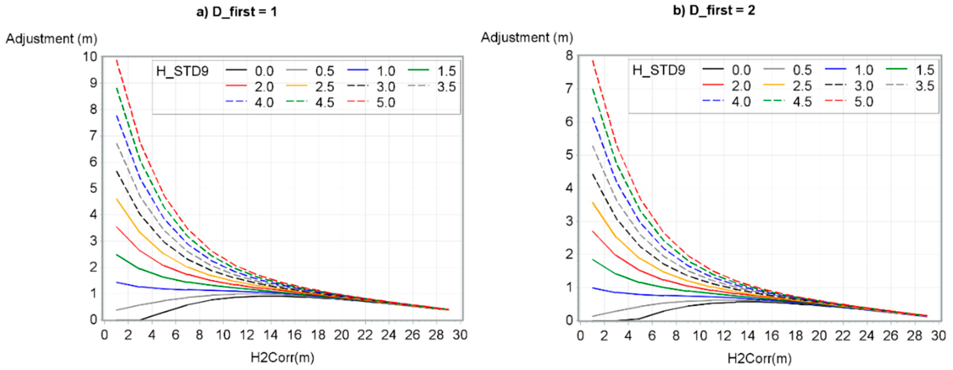
The goals of this study were to propose an adjustment model to correct a DTM bias, and ultimately, to propose an adjustment model to correct CHM bias for a wide range of terrain and acquisition conditions. According to our database and the chosen 1 × 1 m resolution, no variable significantly influenced the DTM correction model and consequently, no models was calculated for DTM. However, three variables were selected for the final CHM adjustment model based on the database in this study and the variables studied: H2Corr, D_first and H_STD9. This model resulted a reduction of the mean bias from 0.70 m to 0.02 m. Also, several notable observations emerged from this study. Among them, the height adjustment decreased as both D_first and H2Corr increased and H_STD9 decreased. The H_STD9 variable had more impact on the adjustments of model for smaller H2Corr values.
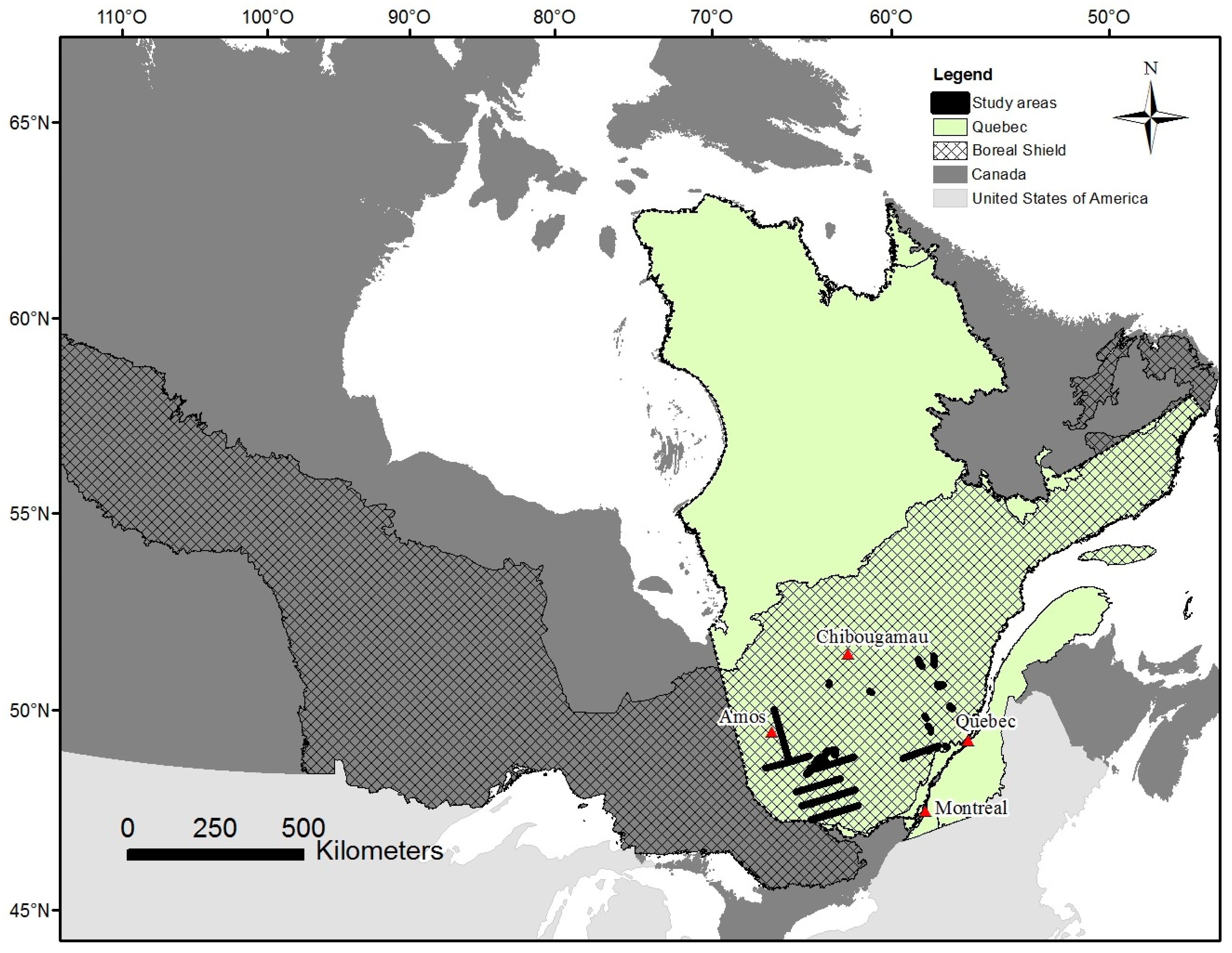
This study was a first attempt to correct LiDAR heights according to a wide range of conditions: 6 sensors studied, diverse angles or pulse densities and study sites covering 3 500 km2 and located on different ecological conditions. Also, results obtained support most of height underestimation studies in the literature. The CHM underestimation correction is a preliminary step to several uses of the CHM such as volume calculation, forest growth models or multi-temporal analysis. For example, before modeling growth with multi-temporal LiDAR data, the underestimation bias on each CHM should be removed; the present work can thus be used in this context.
Finally, its application on various additional data sets in the near future may result in an improvement of models, and may provide better analyses of sensor effects.


