Abstract
With the warming of the global climate, the mass loss of the Greenland ice sheet is intensifying, having a profound impact on the rising of the global sea level. Here, we used Gravity Recovery and Climate Experiment (GRACE) RL06 data to retrieve the time series variations of ice sheet mass in Greenland from January 2003 to December 2015. Meanwhile, the spatial changes of ice sheet mass and its relationship with land surface temperature are studied by means of Theil–Sen median trend analysis, the Mann–Kendall (MK) test, empirical orthogonal function (EOF) analysis, and wavelet transform analysis. The results showed: (1) in terms of time, we found that the total mass of ice sheet decreases steadily at a speed of −195 ± 21 Gt/yr and an acceleration of −11 ± 2 Gt/yr2 from 2003 to 2015. This mass loss was relatively stable in the two years after 2012, and then continued a decreasing trend; (2) in terms of space, the mass loss areas of the Greenland ice sheet mainly concentrates in the southeastern, southwestern, and northwestern regions, and the southeastern region mass losses have a maximum rate of more than 27 cm/yr (equivalent water height), while the northeastern region show a minimum rate of less than 3 cm/yr, showing significant changes as a whole. In addition, using spatial distribution and the time coefficients of the first two models obtained by EOF decomposition, ice sheet quality in the southeastern and northwestern regions of Greenland show different significant changes in different periods from 2003 to 2015, while the other regions showed relatively stable changes; (3) in terms of driving factors temperature, there is an anti-phase relationship between ice sheet mass change and land surface temperature by the mean XWT-based semblance value of −0.34 in a significant oscillation period variation of 12 months. Meanwhile, XWT-based semblance values have the largest relative change in 2005 and 2012, and the smallest relative change in 2009 and 2010, indicating that the influence of land surface temperature on ice sheet mass significantly varies in different years.
1. Introduction
The Greenland ice sheet is the second largest ice sheet in the world after Antarctica, covering an area of 1.73 million square kilometers, and accounting for 10% of total global ice sheet volume [1]. In recent years, with the development of human civilization, the impact of human activities has become more pronounced on the mass balance of the Greenland ice sheet, which highlights serious environmental problems. Its melting rate is much faster than in the previous 20 years, contributing about 0.5 mm/yr to the current global sea level rise of about 3.2 mm/yr [2]. If this acceleration continues, the total sea level rise caused by the melting of the Greenland ice sheet will reach about 9 cm by 2050 [3]. Therefore, the mass change of the Greenland ice sheet is of great significance to the study of global climate change, sea level change, and related fields; then, it is particularly important to understand the spatial–temporal distribution characteristics of ice sheet mass changes in Greenland, and especially its influencing factors.
In March 2002, the Gravity Recovery and Climate Experiment (GRACE) Satellite, launched by the Center for Space Research (CSR), made it possible to monitor the mass balance of the Greenland ice sheet. GRACE consists of two polar orbiting satellites. By detecting the distance between them, we can observe the spatial–temporal variation of the Earth’s gravity field, and then obtain the redistribution of the Earth’s surface mass [4,5,6,7,8,9]. In addition, the spatial resolution of the global gravity field is estimated to be several hundred kilometers and the temporal resolution is one month. At present, GRACE observational data have been well applied in many application fields, such as monitoring surface drought events [10,11,12], groundwater depletion [13,14,15], total water storage change [16,17], and glacier melting [18,19]. Among them, in terms of glacier melting, it is helpful to understand the impact on thermohaline circulation in the Atlantic Ocean. Murray found that the large freshwater input from the Greenland ice sheet may weaken or destroy the “thermo-salt” cycle of marine saltwater, thereby seriously altering the climate of the Northern Hemisphere [20]; Yang et al. estimated new heat and salt flows from the North Atlantic to the Labrador Sea using updated GRACE satellite data, and suggested that the changes in Labrador Sea Water Density (LSW) might be related to the weakening of the Atlantic Meridional Overturning Circulation (AMOC) [21]. In addition, it also plays an important role in the study of the mass change of the Greenland ice sheet.
Some scholars took glacier dynamics into account when they studied the Greenland region, and compared the differences of glacier sheet quality monitoring with GRACE through the climate model and ice sheet model simulation. Alexander et al. [22] found that some areas showed significant differences in peak values times in the annual cycle of mass change on sub-ice-sheet-wide scales, by GRACE with the simulation model; Schlegel et al. [23] found that hydrological and ice–ocean interaction processes should be considered in the model with relatively high temporal resolution (from month to season) to achieve an accurate estimation of Greenland’s mass balance; Xu et al. [24] found that the approximate mass balance between GRACE and input–output method (IOM) is consistent in most Greenland Ice Sheet regions, and the difference in the northwest may be due to underestimating the uncertainty of IOM solutions; Flowers [25] found that about 60% of Greenland’s mass loss in 1991–2015 is attributed to surface mass balance, the net difference between melting and snowfall. The remaining 40% is attributable to dynamic mass loss or uncompensated ice flowing into the ocean.
However, some scholars did not consider glacier dynamics in the process of ice sheet mass analysis. They used different institutions and data sources to study the trend and acceleration of mass change over Greenland’s entire ice sheet over different periods of time. For example, Velicogna et al. [26,27,28] earlier used GRACE data to study the mass balance of Greenland ice sheet, which concluded that the total melting rate of the Greenland ice sheet showed an increasing trend of 248 ± 36 km3/a, and an acceleration of −30 ± 11 Gt/yr2; Ramilli et al. [29] estimated that the melting rate of the Greenland ice sheet was −109 ± 9 Gt/a from 2002 to 2005; Slobbe et al. [30] used GRACE post-processing data to compare Greenland ice sheet mass changes from four different organizations. The results indicated that the different data sources caused different results; Baur et al. [31] explored the annual average Greenland ice sheet melting with a rate of 162 ± 11 km3/a through GRACE RL04 data during 2002–2008; Joodaki et al. [32] found that the mass of the Greenland ice sheet melted at the rate of −166 ± 20 Gt/a and the acceleration of melting was −32 ± 6 Gt/a by GRACE RL04 data from 2002 to 2011; Lu Fei et al. [33] found that the melting speed and acceleration of the ice sheet were −157.8 ± 11.3 Gt/a and −17.7 ± 4.5 Gt/a2, respectively, through GRACE RL05 data from 2003 to 2012. In addition, the melting rate significantly increased after 2010, from −132.2 Gt/a in 2003–2009 to −252.5 Gt/a in 2010–2012; Forsberg et al. [34] concluded that the mass change rate of the Greenland ice sheet was 265 ± 25 Gt/a, and the correlation coefficient was 0.72 with the global mean sea level change. In addition, some scholars studied ice sheet mass trends in different regions of Greenland. Chen et al. [35,36] reported that the mass change rate of Greenland ice sheet was −239 ± 23 km3/yr from April 2002 to November 2005. In addition, its decrease rate increased in the northwest and tended to be balanced in the southeast between 2007 and 2009; Wouter et al. [37] found that the overall mass change rate of the Greenland ice sheet was −179 ± 25 km3/yr on a smaller scale from February 2003 to January 2008 and the greatest mass loss occurred in the southeastern coast (279 Gt) and the northwest coast (328 Gt) in the summer of 2005 and 2007; Zhu Chuandong et al. [38] found that the annual total melting amount of the Greenland ice sheet was 188 ± 10 km3/a during 2002–2011, and the melting area mainly concentrated in the southeast and northwest of the ice sheet; Shamshiri et al. [39] used GRACE RL05 data to conclude that the peak loss of ice mass was −15 cm/yr in the southeast and northwest of Greenland, and loss acceleration was −2.5 cm/yr2 in the southwest during 2003–2014.
Previous studies not only covered a relatively short period, but also mainly focused on the trend of time series, so there were few studies on the significant distribution of spatial trends and the driving factors of ice sheet mass loss. In this paper, we used longer and the latest time series GRACE RL06 data from January 2003 to December 2015 to invert the mass balance of the Greenland ice sheet, and analyze the change trend of ice sheet mass in Greenland. Then, the spatial–temporal variations of the Greenland ice sheet mass were analyzed by using the empirical orthogonal function (EOF) decomposition method. Finally, the common power, relative phase, and correlation of the time series of the Greenland ice sheet mass change and land surface temperature were derived by using continuous wavelet transform (CWT) and cross wavelet transform (XWT) in a time-frequency domain. The research results will help us to macroscopically understand the relationship between ice sheet mass change and land surface temperature in Greenland, which is of great significance for understanding global climate change.
2. Study Area and Data
2.1. Study Area
Greenland is the third largest country of North America and the largest non-continental island in the world [40] (see Figure 1). It lies between longitudes 11° and 74°W, and latitudes 59° and 83°N. In addition, Greenland is bordered by the Greenland Sea to the east, the Arctic Ocean to the north, Baffin Bay to the west, and the North Atlantic Ocean to the southeast. Meanwhile, Iceland is located in the southeast of Greenland in the Atlantic Ocean. Including other offshore minor islands, the total area of Greenland is 2,166,086 km2 (836,330 sq mi). Among them, the Greenland ice sheet has a volume of about 2,850,000 km3 (680,000 cu mi) and covers 1,755,637 km2 (677,855 sq mi) (81%) [41].
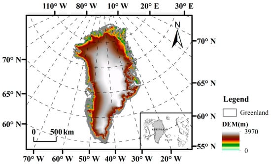
Figure 1.
Map and topography of the Greenland in this study.
2.2. GRACE Data
In this study, we use monthly GRACE data that are processed by the (CSR), University of Texas in Austin, to investigate Greenland ice sheet mass change. The CSR RL05 Level-2 data products are available for data spanning from April 2002 through July 2015, and it does not cover the remaining months of 2015. However, the latest release of GRACE Level-2 RL06 data (http://icgem.gfz-potsdam.de/grace/Level-2/CSR/RL06) covers the whole study period, and has some advantages in spatial resolution, accuracy, and periodic variation characteristics compared with RL05 [42,43]. So, we used CSR RL06 data up to a degree (l) and order (m) 60 in the form of spherical harmonics to study, which includes 142 monthly datasets from January 2003 to December 2015, and compensated for missing data with linear interpolation. Then, one can evaluate monthly local changes of the Earth’s surface mass by using the time-varying gravity spherical harmonic coefficients provided by GRACE [4], with a time resolution of one month, and spatial resolution of 1° × 1°:
where is terrestrial water storage change (surface density variation), a, , θ, , , , are the equatorial radius of the Earth (6377 km), mean density of Earth (5517 kg/m3), latitudes, longitudes, love numbers of degree l with = 60 [44,45], and coefficients changes of the normalized complex spherical harmonic (Stokes’ coefficients), respectively. Meanwhile, is the fully normalized Legendre function of degree l and order m.
In order to eliminate the influence of Earth’s long period and average gravity field, the spherical harmonic coefficients changes are relative to the mean of the 142 monthly solutions. In data processing, the Degree 2 coefficients provided by SLR were used to replace C20 terms based on GRACE orbital solution [46], the degree 1 coefficients provided by Swenson et al. [47] were used to correct the variation terms of Earth’s center of mass (i.e., S11, C11, and C10). Because GRACE observations cannot separate the effects of Glacial Isostatic Adjustment (GIA), the GIA model of Geruo et al. [48] was used to deduct its effects on GRACE observations.
In addition, due to the combined effects of satellite orbit error, ocean–atmosphere model error and the correlation error of the spherical harmonic coefficient of Earth’s gravity field, there are obvious north–south “stripes” error and high frequency error [49] in the inversion of surface mass changes by using Formula (1). Considering the limitation of single filter, this paper used improved P4M6 de-correlation filter to remove north–south “stripes” errors [50], and used a Gaussian filter weight function with a 250 km radius to smooth the noise of the high-order spherical harmonic coefficient [51]. The calculation model is
where is a Gaussian-averaging kernel function related to order, and r is the Gaussian filter smooth radius [4].
Finally, we note that the use of spherical harmonic coefficients of a finite order and spatial filtering leads to ‘leakage’ errors in data processing. However, scale factor 1.95, which was calculated by Velicogna and Wahr [22] could be used to minimize the combined signal leakage and measurement error. In addition, in order to evaluate ice sheet mass changes, surface mass anomalies can be calculated by integrating over the area of specific, since is interpreted as the equivalent water height (i.e., in mm), in that is the density of water (10 × 103 kg/m3). The ice sheet mass variation of Greenland can thus be given as [4]
where θ, λ, and dA are the latitudes, longitudes, and surface element, respectively. In addition, is a region smoothing kernel function, which can be used to accurately evaluate the regional variation of ice sheet mass in Greenland.
2.3. Land Surface Temperature data
GHCN CAMS (Fan et al., 2008) [52] data were downloaded from the website (http://www.esrl.noaa.gov/ psd/data/gridded/tables/.temperature.html) of the National Oceanic and Atmospheric Administration (NOAA), which is a high resolution (0.5° × 0.5°) analyzed global land surface temperature (LST) from 1948 to near present. In this study, GHCN CAMS data were used to study the relationship between ice sheet mass change and land surface temperature in Greenland.
3. Methods
3.1. Theil–Sen Median Trend Analysis
Theil–Sen median trend analysis is a robust non parametric statistical trend calculation method proposed by Hirsch and Slack [53] and Kumar and Saharia [54], which can reduce the influence of abnormal values [55]. For example, this method can calculate the slope of equivalent ice sheet mass from GRACE and temperature changes to analyze trends. The formula is
where , i, and j denote the slopes, and time points, respectively. In addition, and are values at the points of j and i, respectively. The negative value means a decreasing trend, and the positive value means an increasing trend [53].
3.2. Mann–Kendall (MK) Trend Test
The nonparametric M–K test is widely used for trend analysis and significance test of hydrometeorological elements such as rainfall, temperature, and runoff. It has a simple structure, convenient calculation and is not disturbed by a few abnormal values [56]. Statistic S could be obtained based on Equations (1) and (2) [57]
where n is the number of data sets, xj and xi are values at jth and ith points, and sign is a sign function. Then, the M–K statistic, Z, is calculated as
Given a significant level of α, when > , there is a significant change in the study sequence at the level of α. The confidence limit was α = 0.05 in this study, which means |Z| > = 1.96.
3.3. Rotated EOF Method
Empirical orthogonal function analysis is also called principal component analysis or feature vector analysis. It can be used to analyze the variance contribution of different components for extracting the spatial–temporal feature of TWS [58]. The details are
where n and p denote the number of space point, the time period, respectively. In addition, the covariance matrix C of time series is obtained and orthogonally decomposed as
where , the orthogonal decomposition of space domain can be obtained by calculating the feature vector of , and the EOF value can then be obtained by normalizing the decomposition. In addition, the principal component Z can be calculated in the time series.
3.4. Continuous and Cross Wavelet Transform
Firstly, we briefly describe the CWT. The CWT definition of time series (Xn, n = 1, 2, ⋯, N) is [59]
where is the wavelet coefficient, s is the wavelet scale, and are the mother wavelet function and the time scale, respectively, and and n′ represent the normalization factor and the reversed time, respectively. The idea of wavelet transform is that the wavelet as a band-pass filter is applied to time series where the characteristic period of the filter is linearly related to the wavelet scale.
XWT is a new signal analysis technology that combines cross-spectrum analysis with wavelet transform, and studies the relationship between two time series from multi-time scales in the time–frequency domain. Temperature is a well-known trigger for ice sheet melting. Hence, XWT was used to analyze Greenland ice sheet mass changes and temperature time series, which can reveal the regions in which two nonlinear time series with a consistent phase relationship with high common power. The cross wavelet transform of two time series Xn and Yn is given as [60,61,62]
where WY* denotes a complex conjugation of WY. The cross wavelet power spectrum is defined as |WXY|, and the complex argument of WXY can be seen as the local relative phase between Xn and Yn in time–frequency domain. While the larger the |WXY| value, indicating that Xn and Yn have a common high-energy region, which significantly correlates them with each other. More details about Cross Wavelet Power Spectrum test and phase difference calculation are given by Grinsted et al. [59] and are not repeated here.
In analysis, we use the circular mean of the phase and XWT-based semblance to quantify the phase relationship and correlation between two time series. The circular mean of a set of angles (αi, i = 1, 2, …, N) is defined as
We can use circular standard deviation to qualify the scatter of angles around the mean. The XWT-based semblance is defined as [63]
The range of the ρ value is −1 to 0 to 1, which is expressed as negative correlation, irrelevant correlation and positive correlation, respectively. Among them, the closer the value of ρ is to 1, the greater the correlation. In this analysis, we compare the two time series by using XWT-based semblance.
4. Results and Discussion
4.1. Time Variation Analysis
4.1.1. Time Series and Change Trends
For Greenland, we estimated the total ice sheet mass change for each month. As it is shown in Figure 2, the time series variation of monthly Greenland ice sheet mass was estimated in Gt. With the least squares estimate, we fit a linear trend in a mass loss of −268 ± 12 Gt/yr and a quadratic trend in an acceleration of −11 ± 2 Gt/yr2 in 2003–2015, as was done in most previous studies. We use a quadratic form to obtain a trend of −195 ± 21 Gt/yr for the Greenland ice sheet between 2003 and 2015. The uncertainties of the data results (±12, ±2, and ±21) include contributions from the gravity field error, signal leakage effects, truncation error, GIA correction, and the statistical uncertainty of the fit. Mass loss increases with time in a relatively consistent pattern from 2003 to 2012, and a sudden decline in the time series could be observed in 2012. This was followed by a relatively stable mass loss in the next two years after 2012, and then continued in a decreasing trend. The above results are basically consistent with those obtained by researchers using GRACE data in recent years [27,28,33,36,39,64]. However, the time series of the results of this study are longer than those of previous studies, especially the trend of change in 2015 relative to 2014, and their different values are due to different data sources, time series, and post-processing methods.
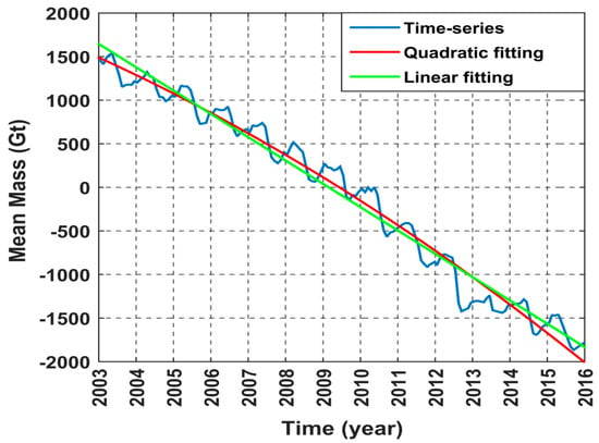
Figure 2.
Monthly mass change of Greenland from January 2003 to December 2015 estimated based on the GRACE solution of the CSR processing center. The blue line, green line and red curve represent the mass change of the time series, and the best fitting of linear and quadratic trend, respectively.
Then, we used the adjusted R-squared () of the data fit to investigate which of the quadratic or linear models is more suitable for time series fitting. More details about were computed by Johnson et al. [65] and are not repeated here. Finally, we found that the for the linear model is 0.9713, which is smaller than the 0.9763 value of the quadratic one. The result agrees with those of other researchers [27,32,64].
4.1.2. Monthly Mean and Seasonal Change
In order to investigate ice sheet mass of intra-annual variability, we calculate the monthly and seasonal changes of ice sheet mass in Greenland, respectively, which are shown in Figure 3. Seasonal changes in the ice sheet mass were averaged from the ice sheet mass in the corresponding months.
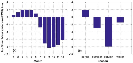
Figure 3.
(a) and (b) represented monthly and seasonal changes in the mass of the Greenland ice sheet from January 2003 to December 2015, respectively.
From Figure 3a, it can be found that positive ice sheet mass change values from GRACE primarily occurred in the first half of each calendar year, while negative ones existed in the second half of each calendar year. The change of ice sheet mass in the whole study area slowly increases between October and April, but decreases between May and September, indicating that the ice sheet mass starts to decrease from May and increase from October. This conclusion is consistent with other scholars, but there are still some differences with regional changes, mainly due to different factors in different regions [22,23,32].
From Figure 3b, it can be found that the average change of ice sheet mass in the whole study area is positive in spring and negative in the rest of the year. Meanwhile, we can also see that the mass of ice sheet decreases from spring to autumn, and then increases from autumn to winter, which is consistent with monthly ice sheet mass changes.
4.2. Spatial Change Analysis
To further study the change trend of ice sheet mass in Greenland from 2003 to 2015, this paper used Theil–Sen median trend analysis and the M–K test to analyze the change trend and significant spatial distribution characteristics of the ice sheet mass (GRACE), and then obtain pixel scale change trends in the whole study area.
In Greenland, we distinguish Greenland into five regions according to the division principle of van den Broeke et al. [66]: (1) southeast (SE), which has a high accumulation, a large number of glaciers at its outlet, a fast speed and a small export; (2) northwest (NW), with highly accumulated and rapidly moving glaciers; (3) southwest (SW), where most glaciers are terrestrial terminals, with the largest melting area; (4) north (N), with a small number of low accumulation, large, and slow-moving glaciers; and (5) northeast (NE), which is similar to N, but glaciers flow through alpine mountains.
Figure 4 shows the spatial distribution of the inter-annual mass loss trend and significance of the Greenland ice sheet from 2003 to 2015, which showed an increasing trend as a whole. The mass loss areas of the Greenland ice sheet are mainly concentrated in the southeastern, southwestern, and northwestern regions, which passed the M–K test of 95% confidence interval. Especially in southeastern Greenland, the trend of mass loss is the largest, with a significant increase rate greater than 27 cm/yr (equivalent water height). In addition, although mass loss rate is less than 3 cm/yr in the northeastern region, it still passes the M–K test of 95% confidence interval, indicating a significant change trend. The above results are consistent with previous studies on regional trends of ice sheet mass loss [28,33].
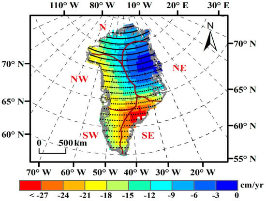
Figure 4.
Spatial distribution of annual change trend of GRACE ice sheet mass in Greenland from 2003 to 2015. Note: Lattice point representation has passed the M–K test of 95% confidence interval.
4.3. EOF Analysis
In order to analyze the spatial distribution characteristics of the mass change of the Greenland ice sheet, the data of GRACE ice sheet mass change were decomposed by EOF from 2003 to 2015. The first second PCA modes account for 98.6% and 0.6% of the variance, respectively, whose accumulative variance is 99.2%; we show the spatial distribution and time-varying characteristics in Figure 5.
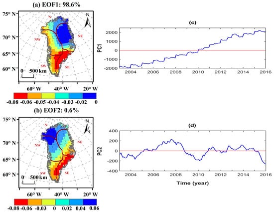
Figure 5.
Spatial distribution (a,b) and time coefficient (c,d) change of the first and second EOF modes. Note: The time coefficients and EOF variables in the figure indicate relative size and are dimensionless.
Figure 5a shows that the overall trend of temporal and spatial variations in Greenland ice sheet mass. EOF1 increases around the southeastern region of Greenland with strong negative values, and the whole region shows negative values, with the northeastern region being the smallest negative value. In terms of time coefficients (i.e., Figure 5c), there is an obvious upward trend from 2003 to 2015, which indicates that the change of ice mass in southeastern Greenland has had a downward trend in the past 13 years. Among them, time coefficients change was obviously weakened in 2010 and 2012, which indicates that the decreasing trend of the ice sheet mass was obvious in 2010 and 2012. At the same time, by comparing ice sheet mass change curve in Figure 2 and the ice sheet mass spatial change significant distribution map in Figure 4, we can also find the corresponding rules.
Figure 5b is the second eigenvector and time coefficient (variance contribution value, 0.6%) derived from the EOF decomposition of GRACE ice sheet mass change in Greenland. As shown in Figure 5b, the southeastern region of Greenland is strongly negative, while the northwestern region is strongly positive, and the other regions are not obvious. In terms of time coefficients (i.e., Figure 5d), there was a significant upward trend from the first half of 2004 to the second half of 2007, and from the first half of 2010 to the first half of 2011, which indicates that the mass loss of the ice sheet in southeastern Greenland was increasing while that in northwest Greenland was decreasing. This result is consistent with that of Lu et al. [33], but the time coefficients from the second half of 2007 to the first half of 2010 and from 2014 to 2015, significantly decreased, which indicates that the loss of ice sheet mass in southeastern Greenland was decreasing while that in northwestern Greenland was increasing. In addition, the change of ice sheet mass in other regions is relatively stable.
4.4. Relationship between Temperature and Ice Sheet Mass
4.4.1. Spatiotemporal Contrastive Analysis
In a time series, in order to eliminate the influence of ice sheet mass and land surface temperature changes within a year, the original time series data were averaged from 13 points, and the Greenland ice sheet mass (GRACE) and land surface temperature change maps were obtained for the study period. Figure 6 shows that the change of GRACE ice sheet mass is obviously opposite to the change of land surface temperature, which reflects the correlation between them to a certain extent. Although there are some differences between them, the main peak–valley characteristics of ice sheet mass changes can be well identified by land surface temperature changes, and the peak–valley value is 1–2 months earlier than the ice sheet mass changes. Overall, the land surface temperature changes show a downward trend (a linear change equation of y= −0.052x + 93) during the study period, which can explain the decline of ice sheet mass to a certain extent.
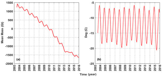
Figure 6.
Annual changes of GRACE ice sheet mass and land surface temperature in Greenland from 2003 to 2015.
Compared with Figure 4 and Figure 7, it can be found that the land surface temperature changes from the southeast to the southwest of Greenland show a significant downward trend, while ice sheet mass loss is significant. In the northwestern region of Greenland, land surface temperature rise is particularly obvious, while the trend of ice sheet mass loss is not the most significant change, which is mainly caused by glacial discharge, temperature, and snow cover [66]. Land surface temperature changes in the northeastern part of Greenland are not significantly decreasing, and the loss change of the ice sheet mass also showed a small but significant reduction. In summary, the change of ice sheet mass and land surface temperature in Greenland are correlated with changes in spatially significant distribution.
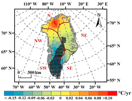
Figure 7.
Spatial distribution of annual change trend of GHCN CAMS land surface temperature in Greenland from 2003 to 2015. Note: Lattice point representation passed the M–K test of 95% confidence interval.
4.4.2. Wavelet Transform Analysis
In order to study the relationship, continuous wavelet transform (CWT) and XWT were used to detect a common power and common relative phase between the time series of ice sheet mass changes and the time series of land surface temperature in Greenland. These wavelet tools can be used to detect local intermittent periodicity [67]. The National Oceanography Center provided the MATLAB code we used [68]. The thick, black contour line indicates that the 95% confidence test was passed, and the thin, black line represents the influence cone (COI), which defines the area not affected by the edge effect. As shown in Figure 8, the energy distribution of the wavelet power spectrum of land surface temperature and ice sheet mass changes is generally consistent, and peak value is mainly concentrated in 10–14 months. In the whole study period, we could see a clear annual cycle, the 12-month spectral energy passed the 95% confidence test, and the shape of the significant band of the wavelet power spectrum in this frequency band is very similar. Results show that the change of land surface temperature and ice sheet mass has a significant 12-month oscillation period.
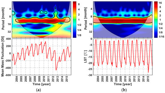
Figure 8.
Continuous wavelet transform with average mass and land surface temperature represented by (a) and (b) from 2003 to 2015.
Similarly, the cross-wavelet power spectrum of land surface temperature and ice sheet mass changes in Greenland could easily be calculated (Figure 9). The arrow direction reflects the relative phase relationship [36] in Figure 9 (with anti-phase pointing left, in-phase pointing right, ice sheet mass changes leading land surface temperature changes by 90°, pointing straight down, and land surface temperature changes leading ice sheet mass changes by 90°, pointing straight up). From Figure 9, the red high-energy region shows that the common power of the two time series was higher for 10–14 months. Since the annual period of 12 month was dominant in the whole observation period, this study mainly focused on the relative phase angles in the 12 month period band, and its average phase angle is −110° ± 6° (6°denotes circular standard deviation).
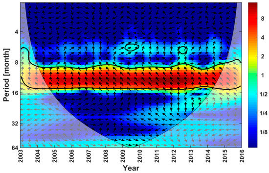
Figure 9.
Cross wavelet transform of ice sheet mass and land surface temperature fluctuations. Arrows indicate relative phase relations, where straight-up arrows represent ice sheet changes, and land surface temperature shows an anti-phase relationship.
Figure 10 describes the XWT-based semblance curve at the period that is closest to one cyclic period year (cpy) outside COI to better show the correlation. The mean XWT-based semblance is −0.34, indicating that the ice sheet mass and land surface temperature changes have an anti-phase relationship in the whole observation period of a significant common power. This correlation is not high. On the one hand, this is because land surface temperature data are surface (3 m) temperature, not ice sheet temperature, so accuracy is relatively low. On the other hand, ice sheet mass change is a combination of increased snow accumulation, increased coastal glacier discharge, and increased surface temperature.
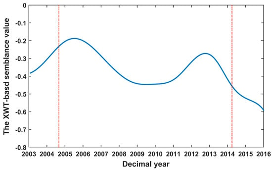
Figure 10.
XWT-based semblance value is the closest to one cpy outside the COI. Red dashed lines represent the COI, which limits the region not affected by edge effects.
5. Conclusions
In this study, the GRACE and GHCN CAMS data were used to investigate the spatiotemporal distribution of ice sheet mass changes and their relationship with land surface temperature in Greenland. GRACE data were used to calculate the mass changes of the Greenland ice sheet from January 2003 to December 2015. The major conclusions of this study are as follows:
From 2003 to 2015, the total mass of the ice sheet decreased steadily at a speed of −195 ± 21 Gt/yr and an acceleration of −11 ± 2 Gt/yr2, which was relatively stable for the two years after 2012, and then continues to show a downward trend. However, in terms of monthly and seasonal variations, the change of ice sheet mass in the whole study area slowly increases between October and April, but decreases between May and September.
According to the inter-annual and spatial variation trend of ice sheet mass and land surface temperature in Greenland, it could be found that ice sheet quality in different regions of Greenland has a significant change trend. For example, Greenland ice sheet mass loss areas are mainly concentrate in the southeastern, southwestern, and northwestern regions, and the southeastern region mass losses at a maximum rate of more than 27 cm/yr (equivalent water height), while northeastern region losses happen at a minimum rate of less than 3 cm/yr. In addition, for EOF results, the variance contribution of the first two eigenvectors is 98.6% and 0.6% respectively, totaling 99.2%. Through the spatial distribution and time coefficients of the first two models, it can be seen that overall ice mass change in Greenland significantly declined in 2010 and 2012. Meanwhile, the ice sheet mass changes in the southeastern and northwestern regions of Greenland showed different significant changes in different periods from 2003 to 2015, while the other regions showed relatively stable changes.
In the time–frequency domain, continuous and cross-wavelet transform were used to study the seasonal relationship between the two time series. We found that land surface temperature and ice sheet mass changes had a significant oscillation periodicity in the 12-month period, and the mean XWT-based semblance value was −0.34, which indicates that ice sheet mass and land surface temperature changes had anti-phase relationships in the whole observation period of a significant common power. In addition, the XWT-based semblance values had the largest relative change in 2005 and 2012, and the smallest relative change in 2009 and 2010, which indicates that the influence of land surface temperature on ice sheet mass significantly varies in different years. However, there are some limitations in the analysis of the relationship between land surface temperature and ice sheet mass changes. It is necessary to take glacier dynamics into account in order to achieve more accurate analysis results in the future.
Author Contributions
Y.B. and J.Y. designed the study and performed the experiments; Y.B. wrote the draft of the manuscript; J.Y. and W.G. supervised the research and revised the manuscript; the other authors are responsible for revision.
Funding
This work was financially supported by National Key R&D Program of China (2018YFC1508603).
Acknowledgments
We are very grateful to Center for Space Research (CSR) for providing RL06 data, National Oceanic and Atmospheric Administration (NOAA) for providing GHCN CAMS data. The authors thank Wei Feng, Vagner G. Ferreira, and Yanping Cao for their help to provide guidance, and would like to thank the editor and three anonymous reviewers for their time and constructive criticism.
Conflicts of Interest
The authors declare no conflicts of interest.
References
- Yang, Y.D.; E, D.C.; Chao, D.B. The Inversion of Ice Mass Change in Greenland Ice Sheet Using GRACE Data. Geomat. Inf. Sci. Wuhan Univ. 2009, 34, 961–964. [Google Scholar]
- Shepherd, A.; Ivins, E.R.; Geruo, A.; Barletta, V.R.; Bentley, M.J.; Bettadpur, S.; Briggs, K.H.; Bromwich, D.H.; Forsberg, R.; Galin, N.; et al. A Reconciled Estimate of Ice-Sheet Mass Balance. Science 2012, 338, 1183–1189. [Google Scholar] [CrossRef]
- Khan, S.A.; Aschwanden, A.; Bjørk, A.A.; Wahr, J.; Kjeldsen, K.K.; Kjær, K.H. Greenland ice sheet mass balance: A review. Rep. Prog. Phys. 2015, 78, 046801. [Google Scholar] [CrossRef]
- Wahr, J.; Molenaar, M.; Bryan, F. Time variability of the Earth’s gravity field: Hydrological and oceanic effects and their possible detection using GRACE. J. Geophys. Res. Solid Earth 1998, 103, 30205–30229. [Google Scholar] [CrossRef]
- Swenson, S.; Wahr, J. Methods of inferring regional surface mass anomalies from Gravity Recovery and Climate Experiment (GRACE) measurements of time-variable gravity. J. Geophys. Res. Solid Earth 2002, 107, 3–13. [Google Scholar] [CrossRef]
- Tapley, B.D. GRACE Measurements of Mass Variability in the Earth System. Science 2004, 305, 503–505. [Google Scholar] [CrossRef] [PubMed]
- Chao, B.F. On inversion for mass distribution from global (time-variable) gravity field. J. Geodyn. 2005, 39, 223–230. [Google Scholar] [CrossRef]
- Wahr, J.M. Time Variable Gravity from Satellites. In Treatise on Geophysics; Elsevier Science: Amsterdam, The Netherlands, 2007; pp. 213–237. [Google Scholar]
- Kumar, S.V.; Zaitchik, B.F.; Peters-Lidard, C.D.; Rodell, M.; Reichle, R.; Li, B.; Jasinski, M.; Mocko, D.; Getirana, A.; De Lannoy, G.; et al. Assimilation of gridded GRACE terrestrial water storage estimates in the North American Land Data Assimilation System. J. Hydrometeorol. 2016, 17, 1951–1972. [Google Scholar] [CrossRef]
- Zhou, H.; Luo, Z.; Tangdamrongsub, N.; Wang, L.; He, L.; Xu, C.; Li, Q. Characterizing drought and flood events over the Yangtze River Basin using the HUST-Grace2016 solution and ancillary data. Remote Sens. 2017, 9, 1100. [Google Scholar] [CrossRef]
- Nie, N.; Zhang, W.; Chen, H.; Guo, H. A Global Hydrological Drought Index Dataset Based on Gravity Recovery and Climate Experiment (GRACE) Data. Water Resour. Manag. 2017, 32, 1275–1290. [Google Scholar] [CrossRef]
- Sun, Z.; Zhu, X.; Pan, Y.; Zhang, J.; Liu, X. Drought evaluation using the GRACE terrestrial water storage deficit over the Yangtze River Basin, China. Sci. Total Environ. 2018, 634, 727–738. [Google Scholar] [CrossRef]
- Hu, K.; Awange, J.L.; Forootan, E.; Goncalves, R.M.; Fleming, K. Hydrogeological characterisation of groundwater over Brazil using remotely sensed and model products. Sci. Total Environ. 2017, 599–600, 372–386. [Google Scholar] [CrossRef]
- Zhong, Y.; Zhong, M.; Feng, W.; Zhang, Z.; Shen, Y.; Wu, D. Groundwater Depletion in the West Liaohe River Basin, China and Its Implications Revealed by GRACE and In Situ Measurements. Remote Sens. 2018, 10, 493. [Google Scholar] [CrossRef]
- Feng, W.; Shum, C.; Zhong, M.; Pan, Y. Groundwater Storage Changes in China from Satellite Gravity: An Overview. Remote Sens. 2018, 10, 674. [Google Scholar] [CrossRef]
- Long, D.; Pan, Y.; Zhou, J.; Chen, Y.; Hou, X.; Hong, Y.; Scanlon, B.R.; Longuevergne, L. Global analysis of spatiotemporal variability in merged total water storage changes using multiple GRACE products and global hydrological models. Remote Sens. Environ. 2017, 192, 198–216. [Google Scholar] [CrossRef]
- Khaki, M.; Forootan, E.; Kuhn, M.; Awange, J.; van Dijk, A.I.J.M.; Schumacher, M.; Sharifi, M.A. Determining water storage depletion within Iran by assimilating GRACE data into the W3RA hydrological model. Adv. Water Resour. 2018, 114, 1–18. [Google Scholar] [CrossRef]
- Flechtner, F. Improved modeling of snow and glacier melting by a progressive two-stage calibration strategy with GRACE and multisource data: How snow and glacier meltwater contributes to the runoff of the Upper Brahmaputra River basin? Water Resour. Res. 2017, 53, 2431–2466. [Google Scholar]
- Ran, J.; Ditmar, P.; Klees, R.; Farahani, H.H. Statistically optimal estimation of Greenland Ice Sheet mass variations from GRACE monthly solutions using an improved mascon approach. J. Geod. 2018, 92, 299–319. [Google Scholar] [CrossRef]
- Murray, T. Climate change: Greenland’s ice on the scales. Nature 2006, 443, 277–278. [Google Scholar] [CrossRef]
- Yang, Q.; Dixon, T.H.; Myers, P.G.; Bonin, J.; Chambers, D.; van den Broeke, M.R. Recent increases in Arctic freshwater flux affects Labrador Sea convection and Atlantic overturning circulation. Nat. Commun. 2016, 7, 10525. [Google Scholar] [CrossRef]
- Alexander, P.M.; Tedesco, M.; Schlegel, N.J.; Luthcke, S.B.; Fettweis, X.; Larour, E. Greenland Ice Sheet seasonal and spatial mass variability from model simulations and GRACE (2003–2012). Cryosphere 2016, 10, 1259–1277. [Google Scholar] [CrossRef]
- Schlegel, N.J.; Wiese, D.N.; Larour, E.Y.; Watkins, M.M.; Box, J.E.; Fettweis, X.; van den Broeke, M.R. Application of GRACE to the assessment of model-based estimates of monthly Greenland Ice Sheet mass balance (2003–2012). Cryosphere 2016, 10, 1–35. [Google Scholar] [CrossRef]
- Xu, Z.; Schrama, E.J.O.; van der Wal, W.; van den Broeke, M.; Enderlin, E.M. Improved GRACE regional mass balance estimates of the Greenland ice sheet cross-validated with the input-output method. Cryosphere 2016, 10, 895–912. [Google Scholar] [CrossRef]
- Flowers, G.E. Hydrology and the future of the Greenland Ice Sheet. Nat. Commun. 2018, 9, 2729. [Google Scholar] [CrossRef]
- Velicogna, I.; Wahr, J. Acceleration of Greenland ice mass loss in spring 2004. Nature 2006, 443, 329–331. [Google Scholar] [CrossRef]
- Velicogna, I. Increasing rates of ice mass loss from the Greenland and Antarctic ice sheets revealed by GRACE. Geophys. Res. Lett. 2009, 36, 158–168. [Google Scholar] [CrossRef]
- Velicogna, I.; Sutterley, T.C.; van den Broeke, M.R. Regional acceleration in ice mass loss from Greenland and Antarctica using GRACE time-variable gravity data. Geophys. Res. Lett. 2014, 41, 8130–8137. [Google Scholar] [CrossRef]
- Ramillien, G.; Lombard, A.; Cazenave, A.; Ivins, E.R.; Llubes, M.; Remy, F.; Biancale, R. Interannual variations of the mass balance of the Antarctica and Greenland ice sheets from GRACE. Glob. Planet Chang. 2006, 53, 198–208. [Google Scholar] [CrossRef]
- Slobbe, D.C.; Ditmar, P.G.; Lindenbergh, R.C. Estimating the rates of mass change, ice volume change and snow volume change in Greenland from ICESat and GRACE data. Geophys. J. Int. 2010, 176, 95–106. [Google Scholar] [CrossRef]
- Baur, O.; Kuhn, M.; Featherstone, W.E. GRACE-derived ice-mass variations over Greenland by accounting for leakage effects. J. Geophys. Res. Solid Earth 2009, 114, 258–266. [Google Scholar] [CrossRef]
- Joodaki, G.; Nahavandchi, H. Mass balance and mass loss acceleration of the Greenland ice sheet (2002–2011) from GRACE gravity data. J. Geod. Sci. 2012, 2, 156–161. [Google Scholar] [CrossRef]
- Lu, F.; You, W.; Fan, D.M. Analysis of Greenland Ice Mass Change Based on GRACE. J. Geod. Geodyn. 2015, 33, 27–30. [Google Scholar]
- Forsberg, R.; Sørensen, L.; Simonsen, S. Greenland and Antarctica Ice Sheet Mass Changes and Effects on Global Sea Level. Surv. Geophys. 2017, 38, 89–104. [Google Scholar] [CrossRef]
- Chen, J.L.; Wilson, C.R.; Tapley, B.D. Satellite gravity measurements confirm accelerated melting of Greenland ice sheet. Science 2006, 313, 1958–1960. [Google Scholar] [CrossRef]
- Chen, J.L.; Wilson, C.R.; Tapley, B.D. Interannual variability of Greenland ice losses from satellite gravimetry. J. Geophys. Res. Solid Earth 2011, 116, B07406. [Google Scholar] [CrossRef]
- Wouters, B.; Chambers, D.; Schrama, E.J.O. GRACE observes small-scale mass loss in Greenland. Geophys. Res. Lett. 2008, 35, 295–296. [Google Scholar] [CrossRef]
- Zhu, C.D.; Lu, Y.; Shi, H.L.; Zhang, Z.Z.; Du, Z.L.; Tu, Y.; Gao, C.C. Quality Changes of the Greenland Ice Sheet Based on GRACE Satellite Data. Hydrogr. Surv. Chart. 2013, 33, 27–30. [Google Scholar]
- Shamshiri, R.; Nahavandchi, H.; Joodaki, G. Seasonal variation analysis of Greenland ice mass time-series. Acta Geod. Geophys. 2017, 53, 1–14. [Google Scholar] [CrossRef]
- Goldhar, C.; Ford, J.D. Climate Change Vulnerability and Food Security in Qeqertarsuaq, Greenland. In Community Adaptation and Vulnerability in Arctic Regions; Springer: Berlin, Germany, 2010; pp. 263–283. [Google Scholar]
- Bamber, J.L.; Ekholm, S.; Krabill, W.B. A new, high-resolution digital elevation model of Greenland fully validated with airborne laser altimeter data. J. Geophys. Res. B Solid Earth 2001, 106, 6733–6745. [Google Scholar] [CrossRef]
- Save, H.; The CSR Level-2 Team. GRACE RL06 Reprocessing and Results from CSR, EGU2018-10697, EGU General Assembly 2012. Available online: https://bit.ly/2Koa1aK (accessed on 3 November 2018).
- Göttl, F.; Schmidt, M.; Seitz, F. Mass-related excitation of polar motion: An assessment of the new RL06 GRACE gravity field models. Earth Planets Space 2018, 70, 195. [Google Scholar] [CrossRef]
- Chao, B.F. The geoid and earth rotation. In Geophysical Interpretations of Geoid; Vanicek, P., Christou, N., Eds.; CRC Press: Boca Raton, FL, USA, 1994. [Google Scholar]
- Farrell, W.E. Deformation of the Earth by surface loads. Rev. Geophys. 1972, 10, 761–797. [Google Scholar] [CrossRef]
- Chen, J.L.; Rodell, M.; Wilson, C.R.; Famiglietti, J.S. Low degree spherical harmonic influences on Gravity Recovery and Climate Experiment (GRACE) water storage estimates. Geophys. Res. Lett. 2005, 32, L14405. [Google Scholar] [CrossRef]
- Swenson, S.; Chambers, D.; Wahr, J. Estimating geocenter variations from a combination of GRACE and ocean model output. J. Geophys. Res. Solid Earth 2008, 113, B08410. [Google Scholar] [CrossRef]
- Geruo, A.; Wahr, J.; Zhong, S. Computations of the viscoelastic response of a 3-D compressible Earth to surface loading: An application to Glacial Isostatic Adjustment in Antarctica and Canada. Geophys. J. Int. 2013, 192, 557–572. [Google Scholar]
- Swenson, S.; Wahr, J. Post-processing removal of correlated errors in GRACE data. Geophys. Res. Lett. 2006, 33, L08402. [Google Scholar] [CrossRef]
- Chen, J.L.; Wilson, C.R.; Blankenship, D.; Tapley, B.D. Accelerated Antarctic ice loss from satellite gravity measurements. Nat. Geosci. 2009, 2, 859–862. [Google Scholar] [CrossRef]
- Han, S.-C.; Shum, C.K.; Jekeli, C.; Kuo, C.-Y.; Wilson, C.; Seo, K.-W. Non-isotropic filtering of GRACE temporal gravity for geophysical signal enhancement. Geophys. J. Int. 2010, 163, 18–25. [Google Scholar] [CrossRef]
- Fan, Y.; van den Dool, H. A global monthly land surface air temperature analysis for 1948–present. J. Geophys. Res. Atmos. 2008, 113, D01103. [Google Scholar] [CrossRef]
- Hirsch, R.M.; Slack, J.R. Non-parametric trend test for seasonal data with serial dependence. Water Resour. Res. 1984, 20, 727–732. [Google Scholar] [CrossRef]
- Jain, S.K.; Kumar, V.; Saharia, M. Analysis of rainfall and temperature trends in northeast India. Int. J. Climatol. 2013, 33, 968–978. [Google Scholar] [CrossRef]
- Yuan, L.H.; Jiang, W.G.; Shen, W.M.; Liu, Y.H.; Wang, W.J.; Tao, L.L.; Zheng, H.; Liu, X.F. The spatio-temporal variations of vegetation cover in the Yellow River Basin from 2000 to 2010. Acta Ecol. Sin. 2013, 33, 7798–7806. [Google Scholar]
- Liu, Z.F.; Wang, Y.C.; Yao, Z.J.; Kang, H.M. Trend and periodicity of precipitation, air temperature and runoff in the Taihu Lake Basin. J. Nat. Resour. 2011, 26, 1575–1584. [Google Scholar]
- Yue, S.; Hashino, M. Temperature Trends in Japan: 1900–1990. Theor. Appl. Climatol. 2003, 75, 15–27. [Google Scholar]
- Yang, P.; Xia, J.; Zhan, C.; Qiao, Y.; Wang, Y. Monitoring the spatio-temporal changes of terrestrial water storage using GRACE data in the Tarim River basin between 2002 and 2015. Sci. Total Environ. 2017, 595, 218–228. [Google Scholar] [CrossRef]
- Grinsted, A.; Moore, J.C.; Jevrejeva, S. Application of the cross wavelet transform and wavelet coherence to geophysical time series. Nonlinear Process. Geophys. 2004, 11, 561–566. [Google Scholar] [CrossRef]
- Jevrejeva, S.; Moore, J.C.; Grinsted, A. Influence of the Arctic Oscillation and El Niño-Southern Oscillation (ENSO) on ice conditions in the Baltic Sea: The wavelet approach. J. Geophys. Res. Atmos. 2003, 108, D214677. [Google Scholar] [CrossRef]
- Xu, C. Investigating Mass Loading Contributors of Seasonal Oscillations in GPS Observations Using Wavelet Analysis. Pure Appl. Geophys. 2016, 173, 2767–2775. [Google Scholar] [CrossRef]
- Guo, J.; Li, W.; Yu, H.; Liu, Z.; Zhao, C.; Kong, Q. Impending ionospheric anomaly preceding the Iquique Mw8.2 earthquake in Chile on 2014 April 1. Geophys. J. Int. 2015, 203, 1461–1470. [Google Scholar] [CrossRef]
- Cooper, G.R.J.; Cowan, D.R. Comparing time series using wavelet-based semblance analysis. Comput. Geosci. 2008, 34, 95–102. [Google Scholar] [CrossRef]
- Gardner, A.S.; Moholdt, G.; Cogley, J.G.; Wouters, B.; Arendt, A.A.; Wahr, J.; Berthier, E.; Hock, R.; Pfeffer, W.T.; Kaser, G.; et al. A Reconciled Estimate of Glacier Contributions to Sea Level Rise: 2003 to 2009. Science 2013, 340, 852–857. [Google Scholar] [CrossRef]
- Johnson, R.A.; Wichern, D.W. Applied Multivariate Statistical Analysis, 5th ed.; Prentice Hall: Upper Saddle River, NJ, USA; Englewood, IL, USA, 2002. [Google Scholar]
- Van den Broeke, M.; Bamber, J.; Ettema, J.; Rignot, E.; Schrama, E.; van de Berg, W.J.; van Meijgaard, E.; Velicogna, I.; Wouters, B. Partitioning recent Greenland mass loss. Science 2009, 326, 984–986. [Google Scholar] [CrossRef]
- Tomás, R.; Li, Z.; Lopez-Sanchez, J.M.; Liu, P.; Singleton, A. Using wavelet tools to analyse seasonal variations from InSAR time-series data: A case study of the Huangtupo landslide. Landslides 2015, 13, 437–450. [Google Scholar] [CrossRef]
- National Oceanography Center N. Crosswavelet and Wavelet Coherence. Available online: http://noc.ac.uk/usingscience/crosswavelet-wavelet-coherence (accessed on 28 November 2018).
© 2019 by the authors. Licensee MDPI, Basel, Switzerland. This article is an open access article distributed under the terms and conditions of the Creative Commons Attribution (CC BY) license (http://creativecommons.org/licenses/by/4.0/).