Article

Local Azimuth Ambiguity-to-Signal Ratio Estimation Method Based on the Doppler Power Spectrum in SAR Images

1
National Key Lab of Microwave Imaging Technology, Beijing 100190, China
2
Institute of Electronics, Chinese Academy of Sciences, Beijing 100190, China
3
School of Electronics, Electrical and Communication Engineering, University of Chinese Academy of Sciences, Beijing 100190, China
*
Author to whom correspondence should be addressed.
Remote Sens. 2019, 11(7), 857; https://doi.org/10.3390/rs11070857
Submission received: 20 February 2019 / Revised: 7 April 2019 / Accepted: 8 April 2019 / Published: 9 April 2019
(This article belongs to the Special Issue Advanced Topics in Remote Sensing)

Abstract

:
In synthetic aperture radar (SAR) images, azimuth ambiguity is one of the important factors that affect image quality. Generally, the azimuth ambiguity-to-signal ratio (AASR) is a measure of the azimuth ambiguity of SAR images. For the low signal-to-noise ratio (SNR) ocean areas, it is difficult to accurately estimate the local AASR using traditional estimation algorithms. In order to solve this problem, a local AASR estimation method based on the Doppler power spectrum in SAR images is proposed in this paper by analyzing the composition of the local Doppler spectrum of SAR images. The method not only has higher estimation accuracy under low SNR, but also overcomes the limitations of traditional algorithms on SAR images when estimating AASR. The feasibility and accuracy of the proposed method are verified by simulation experiments and spaceborne SAR data.

Graphical Abstract

1. Introduction

Due to the limitation of azimuth sampling, the azimuth spectrum of SAR images will be aliased in the process of data acquisition of synthetic aperture radar (SAR) [1]. The aliasing phenomenon of the spectrum is known as azimuth ambiguity [2,3,4]. For spaceborne SAR systems, azimuth ambiguity is highly prone to occur in SAR images [1,5], especially for the SAR ocean images at the sea–land junction. Because the scattering coefficient of the ocean region is quite low, the azimuth ambiguity signal of the land strong-scattering target will form a “ghost” in the low-scattering region of the ocean. The “ghost” will undoubtedly bring false alarms to the detection of marine targets [6].
In SAR systems, the azimuth ambiguity-to-signal ratio (AASR) is an important parameter to measure the influence of azimuth ambiguity signals on SAR images [7,8]. Factors affecting the AASR include azimuthal processing parameters (wavelength, azimuth processing bandwidth, pulse repetition frequency (PRF)) and azimuth antenna pattern (AAP) [9,10]. In general, one or more influencing factors can be controlled for the suppression of the azimuth ambiguity. First, a weighting of the azimuth antenna pattern could be considered when designing a SAR system, thereby the aliased azimuth ambiguity signal energy can be reduced. Moreover, the PRF could be properly set before the acquisition of SAR data. If the SAR image has already been acquired, a reduced Doppler bandwidth could be adopted, or an amplitude weighting of the Doppler spectrum could be applied in the processing [11,12]. However, these processing methods may result in a decrease in azimuth resolution, and even signal energy that is overwhelmed by azimuth ambiguity will be lost. Therefore, it is particularly important to improve the degree of suppression of azimuth ambiguity by estimating the accurate local AASR.
In 2005, Guarnieri proposed the adaptive removal of azimuth ambiguities in SAR images [8], and estimated the AASR in SAR images based on backscatter technique, which is referred to as a backscatter-based (BB) algorithm in this paper. However, this method is limited to the fact that the ambiguity source signal must appear in the focused SAR image. In 2014, Villano, et al. proposed the spectral-based (SB) estimation algorithm of the local AASR in SAR images [13]. This method gets rid of the limitation that the BB algorithm requires that the ambiguity source signal must appear in the focused SAR image. However, the SB algorithm does not consider the effect of the signal-to-noise ratio (SNR) of SAR images on the estimation result when performing local AASR estimation. For most ocean areas, the SNR of the SAR image is relatively low. Therefore, the influence of system noise on the estimation results cannot be ignored.
In order to make up for the shortcomings of the two local AASR estimation methods above, a local AASR estimation method based on the Doppler power spectrum in SAR images is proposed in this paper. The procedure of the proposed method is as follows. Firstly, the relationship between the local AASR and the Doppler power spectrum of local SAR images is derived by analyzing the Doppler spectral composition of the local SAR image. Secondly, the ratio of the left and right blurred positions to the normalized radar cross-section (NRCS) of the main signal position can be estimated by the relationship between the Doppler center spectrum and the edge spectrum, respectively. Finally, the local AASR can be calculated from the ratio of the left and right blurred positions to the NRCS of the main signal position.
The rest of this paper is organized as follows. Section 2 gives the composition analysis of the Doppler spectrum and the theoretical derivation of the proposed method. In Section 3, the feasibility and accuracy of the proposed method are verified by simulation experiments, and the estimation accuracy under different SNRs is given. In Section 4, the proposed method is verified by the real spaceborne SAR data. Finally, conclusions are presented in Section 5.

2. Local AASR Estimation Method Based on the Doppler Power Spectrum

2.1. The Analysis of Local Doppler Power Spectrum Composition

From the SAR imaging theory [14,15], it is well known that the shape of system noise, azimuthal ambiguity, and the backscattering signal present as different patterns in the Doppler spectrum of the SAR raw signal (here, it is supposed that the range match filtering and range cell migration correction have been done), i.e., the system noise power density is a certain constant in the Doppler spectrum, whereas the shape of the Doppler spectrum of the backscattering signal and azimuthal ambiguity depend on the antenna pattern: The backscattering signal and azimuthal ambiguity correspond to the main lobe and side lobe respectively. The Doppler spectrum of the SAR raw signal can be expressed as the following [16,17]:
E [ p ( f , x 0 , y 0 ) ] = n = n = σ ¯ ( x 0 + n D x , y 0 + n D y ) P a ( f f 0 + n F a ) + N 0 F a
where ( x 0 , y 0 ) are the center positions of the area upon which the Fourier transformation is applied; x and y are the coordinates in the flight and look directions respectively, E [ · ] refers to the mathematic expectation, f denotes the Doppler frequency, and p ( f , x 0 , y 0 ) denotes the azimuth power spectrum of the SAR raw signal, in order to simplify the reading, p ( f ) is used instead of p ( f , x 0 , y 0 ) . n is the fuzzy number, P a ( f ) is the power spectrum of an ideal point target with a 0 dB normalized radar cross-section (NRCS) and its shape is determined by the two-way AAP. Further, f 0 is the Doppler centroid, F a refers to the pulse repeat frequency of the SAR system, N 0 is the intrinsic noise floor of the SAR system, σ ¯ ( x 0 + n D x , y 0 + n D y ) is the mean NRCS of the pixels located between ( x 0 + n D x L / 2 , y 0 + n D y ) and ( x 0 + n D x + L / 2 , y 0 + n D y ) ( L is the data length for calculating the Doppler spectrum), D x and D y are the displacements between the position of the azimuth ambiguity signal and the real target position in the flight and look directions, respectively. They can be written as [18]
D x = R λ F a 2 V , D y = λ 2 f 0 F a R 4 V 2
where R is the slant range of the target, λ is the radar wavelength, and V is the velocity of the SAR platform.
Generally, the energy of the first blurred regions in SAR image accounts for at least 85% of the total blur energy [9,19]. Therefore, we only consider the ambiguity energy introduced by the first side lobes of the antenna pattern. Hence, Equation (1) can be simplified to
E [ p ( f , x 0 , y 0 ) ] σ ¯ ( x 0 , y 0 ) P a ( f f 0 ) + σ ¯ ( x 0 + D x , y 0 + D y ) P a ( f f 0 + F a ) + σ ¯ ( x 0 D x , y 0 D y ) P a ( f f 0 F a ) + N 0 F a
Equation (3) indicates that the shape of the averaged power spectrum of backscattering signal, azimuth ambiguity, and system noise are determined by the AAP ( P a ( f ) ) and N 0 .

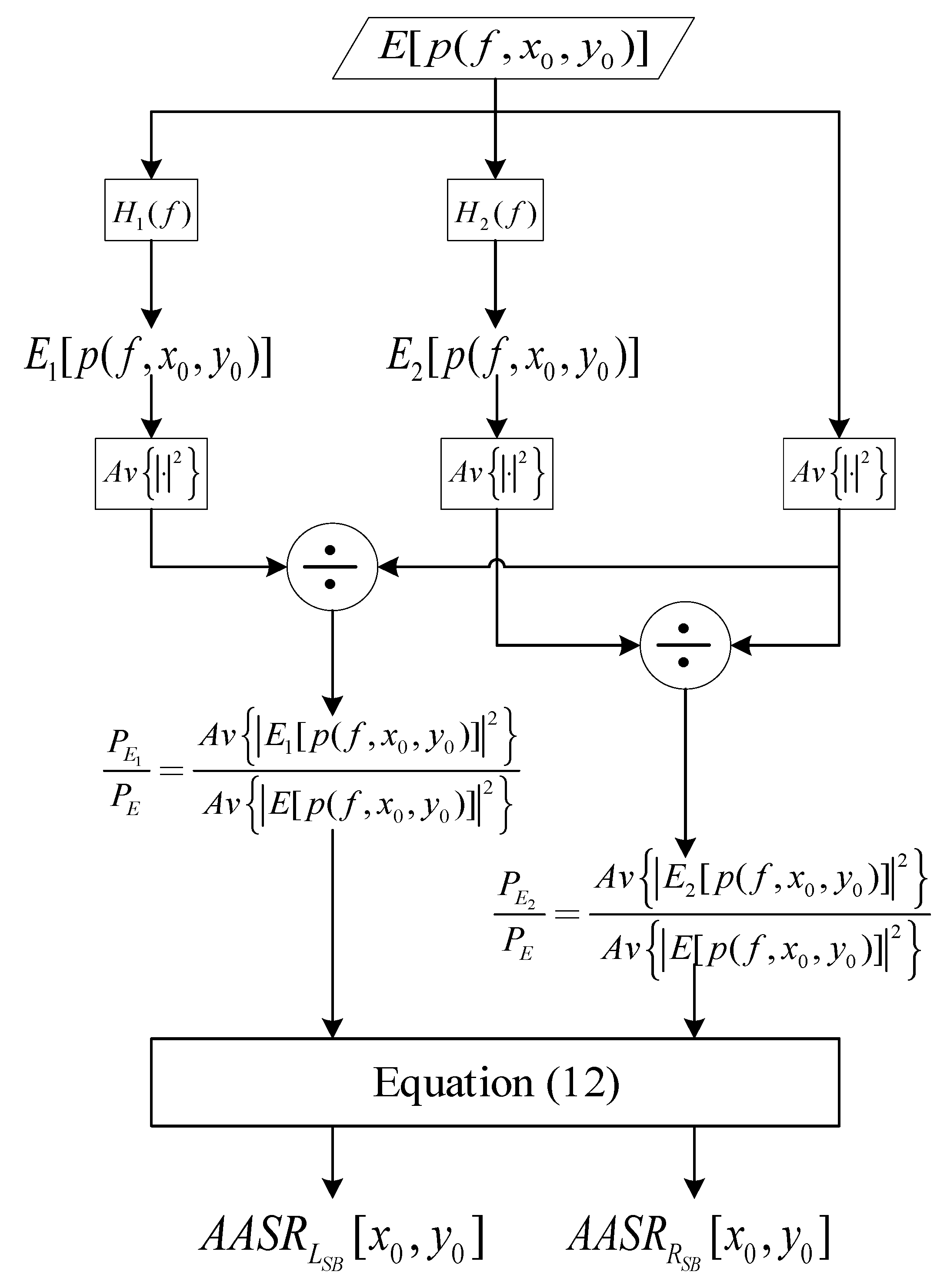
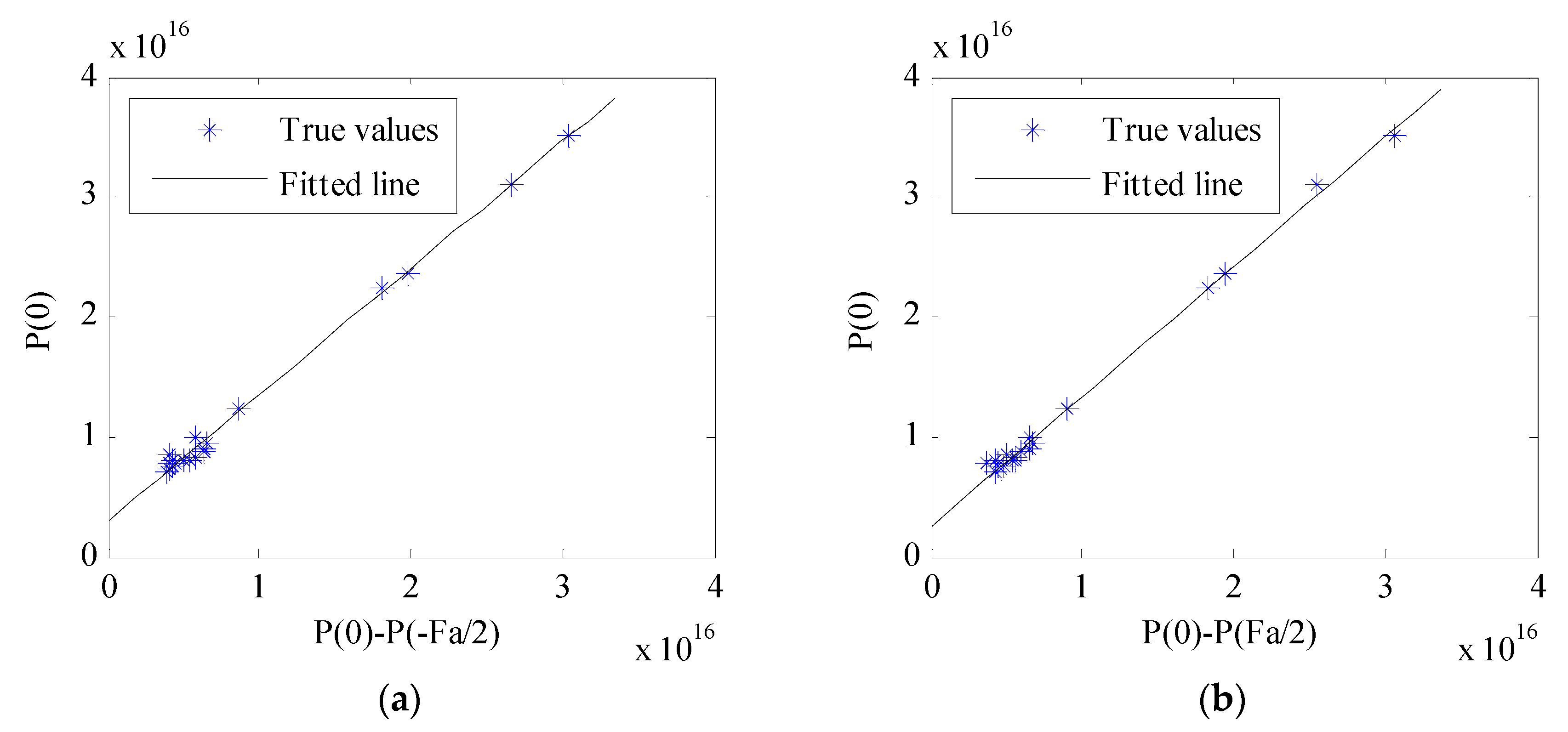
2.2. Methods and Solutions to Estimate the Local AASR from the Doppler Power Spectrum

According to Equation (3), the local AASR can be defined as
A A S R = N A A S R l B d / 2 B d / 2 P a ( f f 0 F a ) d f + N A A S R r B d / 2 B d / 2 P a ( f f 0 + F a ) d f B d / 2 B d / 2 P a ( f f 0 ) d f
where, B d is the azimuthal processing bandwidth. N A A S R l = σ ¯ ( x 0 D x , y 0 D y ) σ ¯ ( x 0 , y 0 ) represents the ratio of the NRCS of the left blurred position to that of the main signal position, while N A A S R r = σ ¯ ( x 0 + D x , y 0 + D y ) σ ¯ ( x 0 , y 0 ) represents the ratio of the NRCS of the right blurred positions to that of the main signal position.
It can be seen from Equation (4) that if we want to estimate the local AASR from the local Doppler power spectrum, N A A S R l and N A A S R r must be estimated first. Therefore, Equation (3) can be expressed as
E [ p ( f , x 0 , y 0 ) ] σ ¯ ( x 0 , y 0 ) [ P a ( f f 0 ) + N A A S R r P a ( f f 0 + F a ) + N A A S R l P a ( f f 0 F a ) ] + N 0 F a
Since the P a ( f ) can be obtained by SAR calibration [20,21], there are only three unknowns ( N A A S R l , N A A S R r and N 0 ) in Equation (5). Therefore, Equation (5) can be simplified by choosing three different frequency points in the Doppler spectrum (for example, f 1 , f 2 , and f 3 ), then the following two linear relationships is derived out.
{ E [ p ( f 1 ) ] = { E [ p ( f 1 ) ] E [ p ( f 3 ) ] } β 1 + N 0 F a E [ p ( f 1 ) ] = { E [ p ( f 1 ) ] E [ p ( f 2 ) ] } β 2 + N 0 F a
where,
{ β 1 = w ( f 1 ) w ( f 1 ) w ( f 3 ) β 2 = w ( f 1 ) w ( f 1 ) w ( f 2 ) , w ( f ) = P a ( f f 0 ) + N A A S R r P a ( f f 0 + F a ) + N A A S R l P a ( f f 0 F a )
The two equations in Equation (6) are linear, in which the constant term depends on the noise floor N 0 , and the linear coefficient β 1 , β 2 depends on N A A S R l and N A A S R r (see Equation (7)). Theoretically, if there are more than two sufficiently averaged Doppler spectra, β 1 , β 2 , and N 0 can be resolved by Equation (6). More Doppler spectra will result in a more precise estimation of β 1 , β 2 and N 0 . To increase the estimation precision, f 1 , f 2 , and f 3 should be selected to make E [ p ( f 1 ) ] E [ p ( f 2 ) ] and E [ p ( f 1 ) ] E [ p ( f 3 ) ] as large as possible while E [ p ( f 2 ) ] and E [ p ( f 3 ) ] as small as possible [17]. Therefore, f 1 = f 0 , f 2 = f 0 F a / 2 , and f 3 = f 0 + F a / 2 are selected in this paper.
In order to simplify reading, the sinc model is selected as the AAP model. Therefore, the AAP can be expressed as
P a ( f ) = sin c 4 ( f b )
Substituting Equation (8) into Equation (7), Equation (7) becomes
{ β 1 = 1 + N A A S R l sin c 4 ( F a b ) + N A A S R r sin c 4 ( F a b ) 1 - sin c 4 ( F a 2 b ) + N A A S R l [ sin c 4 ( F a b ) - sin c 4 ( 3 F a 2 b ) ] + N A A S R r [ sin c 4 ( F a b ) - sin c 4 ( F a 2 b ) ] β 2 = 1 + N A A S R l sin c 4 ( F a b ) + N A A S R r sin c 4 ( F a b ) 1 - sin c 4 ( F a 2 b ) + N A A S R l [ sin c 4 ( F a b ) - sin c 4 ( F a 2 b ) ] + N A A S R r [ sin c 4 ( F a b ) - sin c 4 ( 3 F a 2 b ) ]
β 1 , β 2 b F a are the known amount, N A A S R l and N A A S R r are unknown. The above equation is a linear equation system with two unknowns, which can be expressed in the form of a matrix operation.
( p 11 p 12 p 21 p 22 ) ( N A A S R l N A A S R r ) = ( q 1 q 2 )
where, { p 11 = sin c 4 ( F a b ) β 2 sin c 4 ( F a b ) + β 2 sin c 4 ( 3 F a 2 b ) p 12 = sin c 4 ( F a b ) β 2 sin c 4 ( F a b ) + β 2 sin c 4 ( F a 2 b ) p 21 = sin c 4 ( F a b ) β 1 sin c 4 ( F a b ) + β 1 sin c 4 ( F a 2 b ) p 22 = sin c 4 ( F a b ) β 1 sin c 4 ( F a b ) + β 1 sin c 4 ( 3 F a 2 b )   q 1   = β 2 β 2 sin c 4 ( F a 2 b ) 1   q 2   = β 1 β 1 sin c 4 ( F a 2 b ) 1 .
By performing a matrix operation on Equation (10)
( N A A S R l N A A S R r ) = ( p 11 p 12 p 21 p 22 ) 1 ( q 1 q 2 )
The local AASR can be obtained by substituting the estimation result into Equation (4). The sidelobe weight of the azimuth weighting filter is then appropriately adjusted by the estimated local AASR, so that the azimuth ambiguity signal energy can be more accurately suppressed.

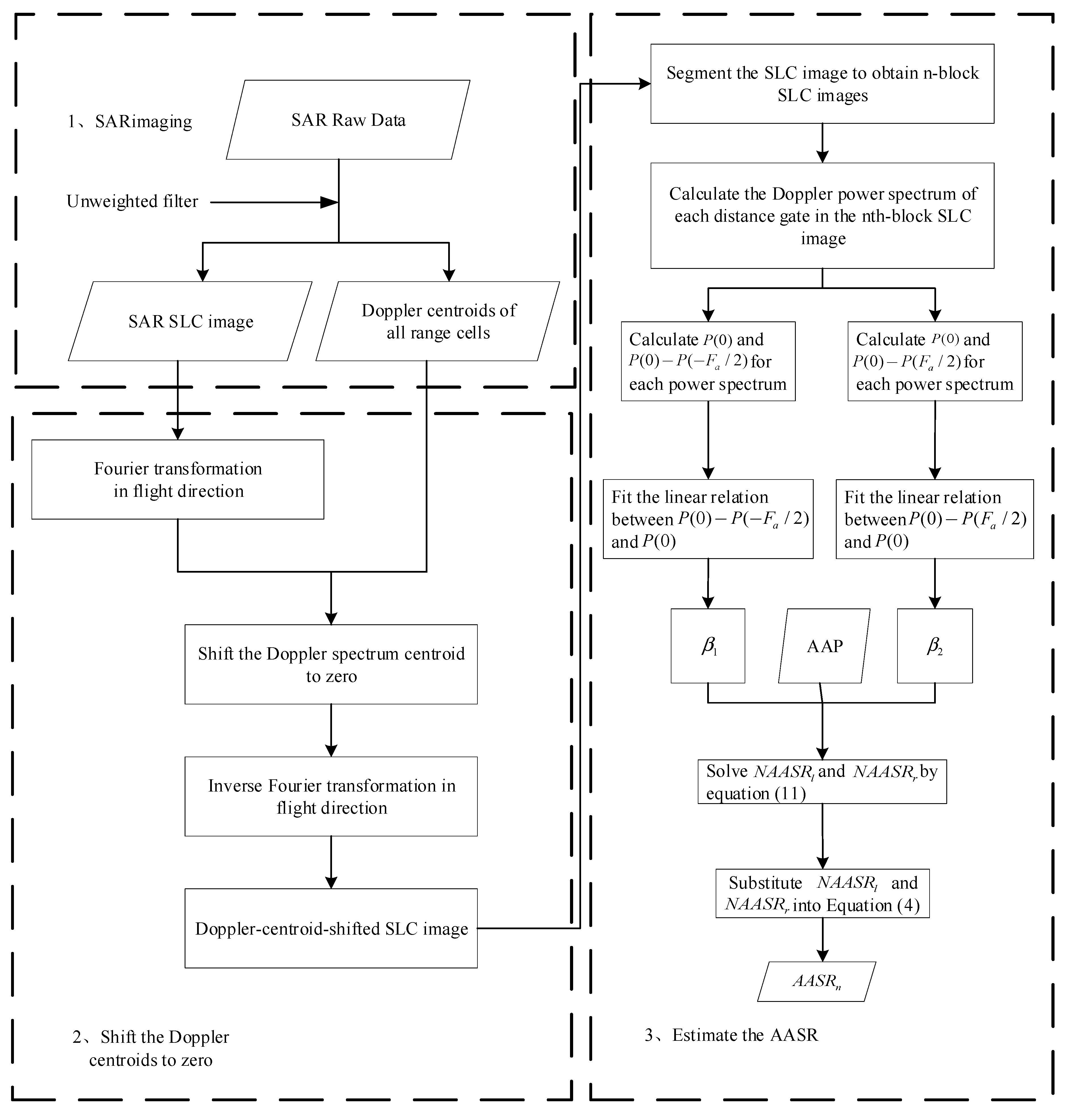
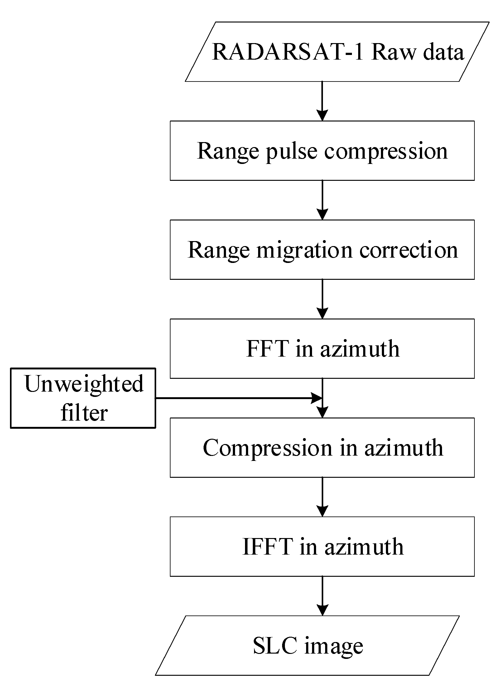
2.3. The Flow Chart of the Proposed Method

The proposed method starts with the SAR raw data. SAR images obtained by traditional commercial spaceborne radars typically use weighted filtering in the azimuth. However, this processing can result in a loss of the true NRCS of the target, which does not apply to the proposed method in this paper. In order to preserve the most accurate NRCS of the target, an unweighted azimuthal matching filter must be applied to the SAR raw data. The procedure of the proposed method is as follows.
In the first step, the SAR data is imaged using the unweighted azimuth filter to obtain a single-look complex (SLC) image. In the second step, the Doppler center frequency must be estimated from the SLC image [22,23,24], and then the Doppler centroids of the SLC image are shifted to the zero-frequency. In the third step, the corrected SLC image is segmented into n-block local SLC images, and the size of each image is R r × R a (range multiplied by azimuth). An average Doppler power spectrum is obtained for each range gate of each image. We assume that the average Doppler power spectrum is E [ p ( f ) ] = P ( f ) . By the statistics of the linear relationship between the Doppler center spectrum and the two edge spectra in each Doppler power spectrum, two different linear factors β 1 and β 2 can be obtained. The ratio of the NRCS of the left and right ambiguity signal position to that of the main signal position can then be obtained by solving the binary equations. Finally, the AASR of the local SLC image can be obtained by substituting the estimation result into Equation (4).
The proposed method is summarized in Figure 1.

3. Verification Based on the Simulation Experiment

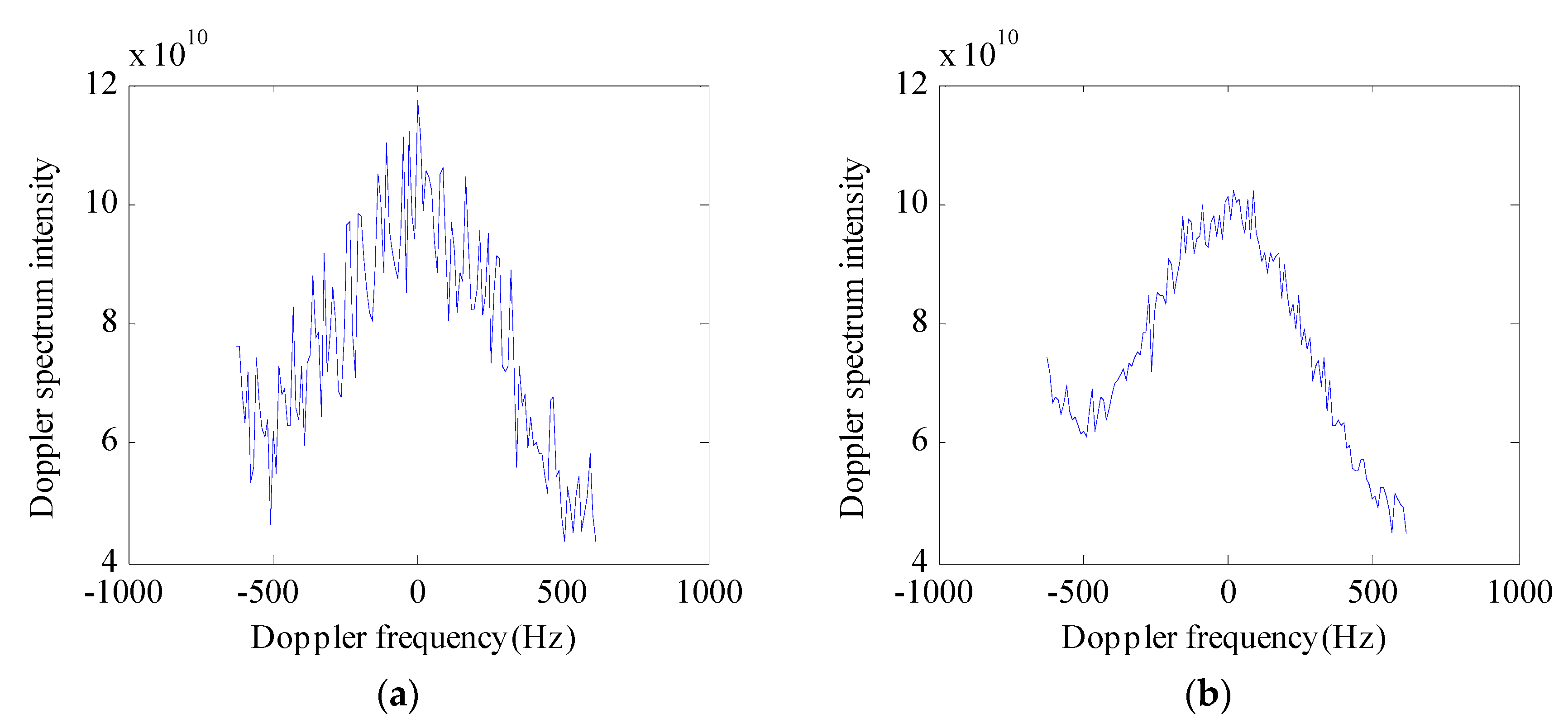
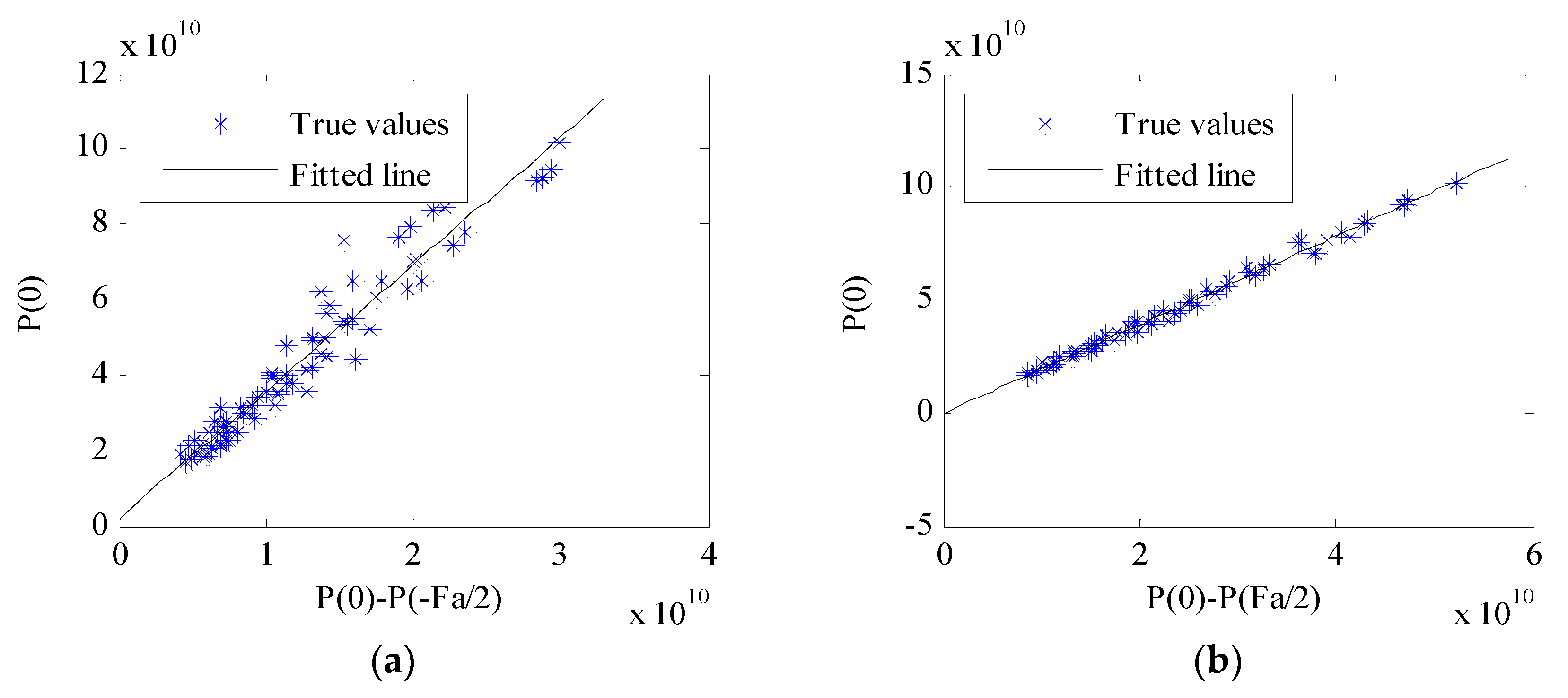
3.1. The Simulation Experiment of the Proposed Method

Section 2 describes the principle of the proposed method. In this section, the method is verified by simulation experiments. The parameters of the simulation experiment are shown in Table 1.
According to the parameters in Table 1, the simulated Doppler power spectrum is shown in Figure 2.
It can be seen from Figure 2 that because the ambiguity energy of the left and right ambiguity positions is different in the simulation process, the left and right edge spectra of the simulated Doppler spectrum are asymmetrical. Using the same method as Figure 2 to generate several Doppler power spectra to form a two-dimensional frequency domain image. The statistical relationship between P ( 0 ) P ( F a / 2 ) and P ( 0 ) from the simulated two-dimensional image is shown in Figure 3a, and the statistical relationship between P ( 0 ) P ( F a / 2 ) and P ( 0 ) from the simulated two-dimensional image is shown in Figure 3b.
The variables β 1 and β 2 in Equation (7) are the slope of the fitted lines in Figure 3a,b, respectively. The variable N A A S R l and N A A S R r can then be solved by Equations (9)–(11). Substituting the result into Equation (4), we can obtain the true local AASR. The comparison between the estimation results of the proposed method and the estimation results of the two traditional algorithms (SB algorithm and BB algorithm) is shown in Table 2.
As can be seen from Table 2, when the SNR is 5 dB and the local AASR is −9.435 dB, the N A A S R l and N A A S R r estimated by the proposed method are very close to the true values. In addition, as far as the local AASR estimation results are concerned, the estimation result of the proposed method is closer to the true value.

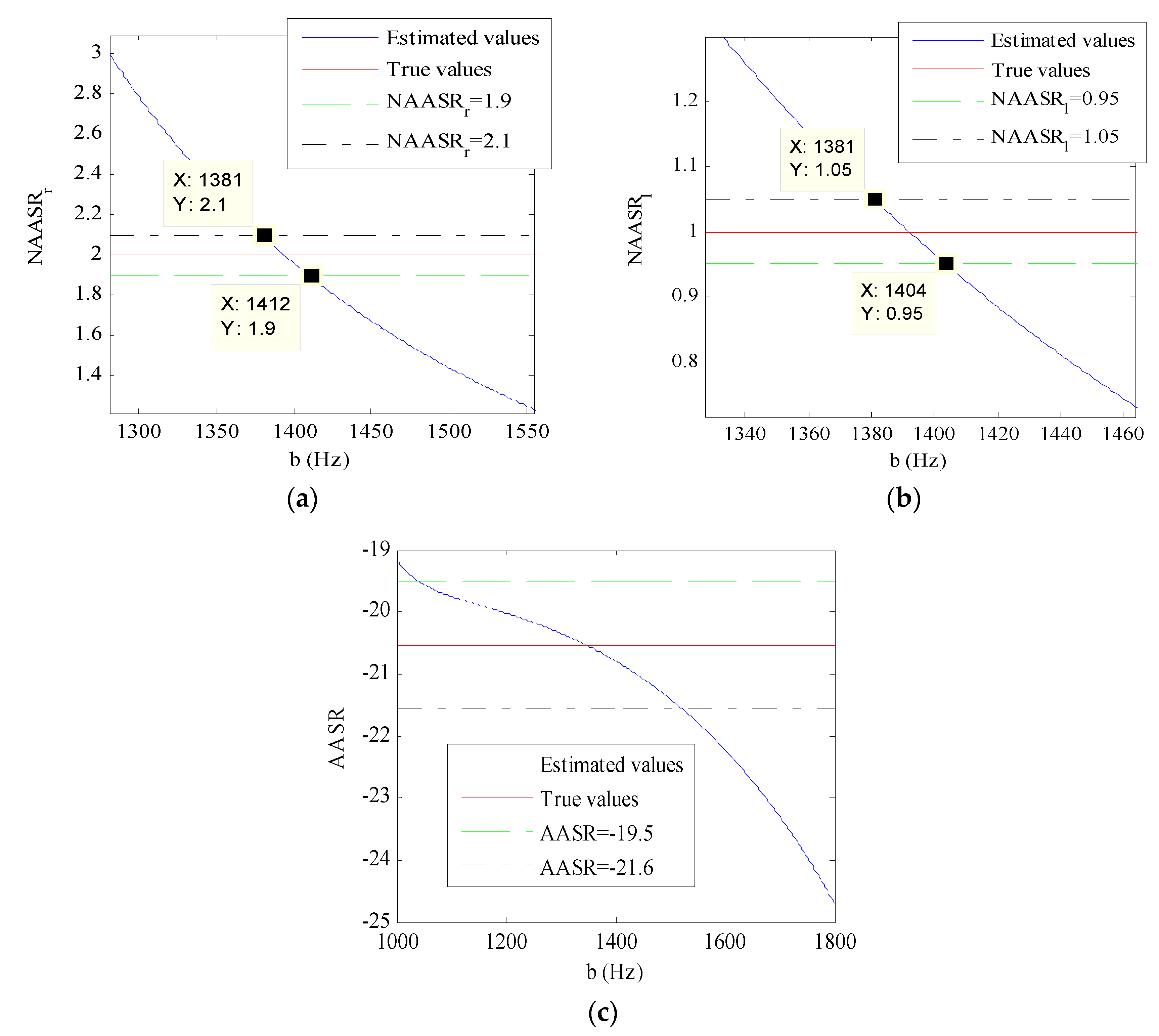
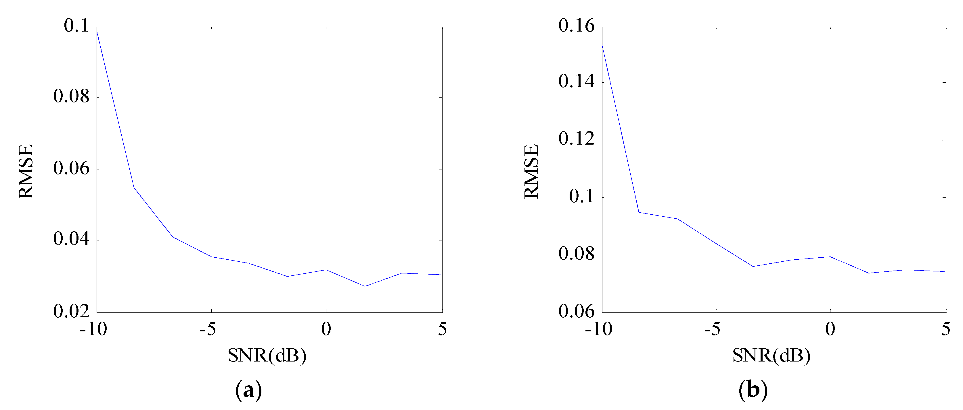
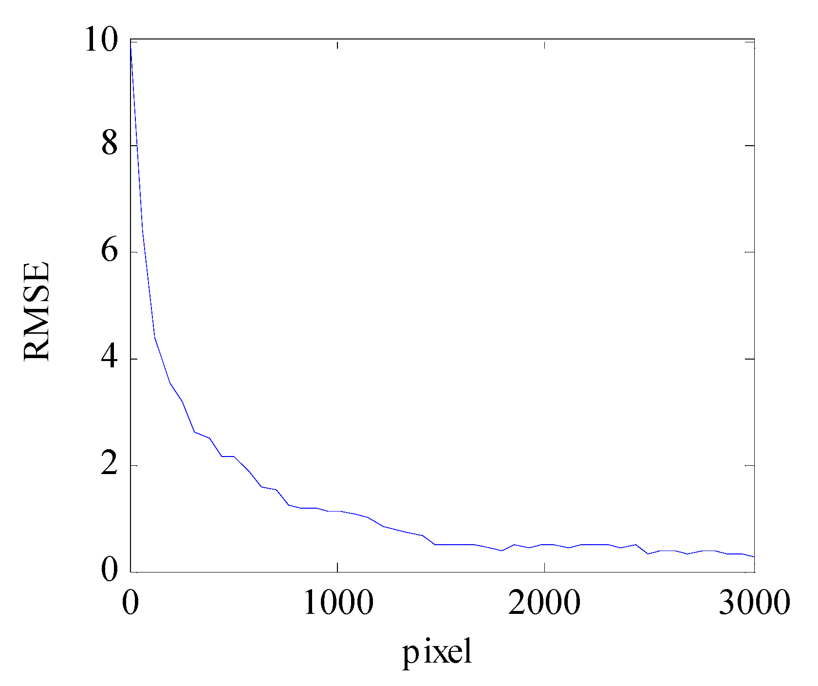
3.2. The Influence of the SNR of SAR Image on Estimation Accuracy

In order to analyze the estimation accuracy of the proposed method under different SNR conditions, 200 random Monte Carlo experiments are performed. The curve of the root mean squared error (RMSE) of the estimated result changes with SNR is simulated. The results are shown in Figure 4.
It can be seen from Figure 4 that as the signal-to-noise ratio increases, the RMSE of the N A A S R l and N A A S R r estimation results gradually decrease. This illustrates the feasibility of the proposed method in this paper.

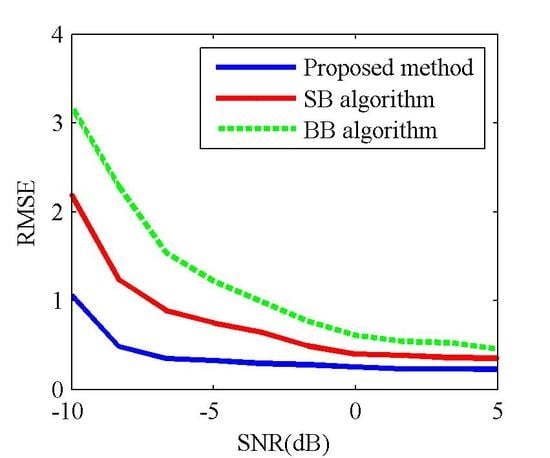
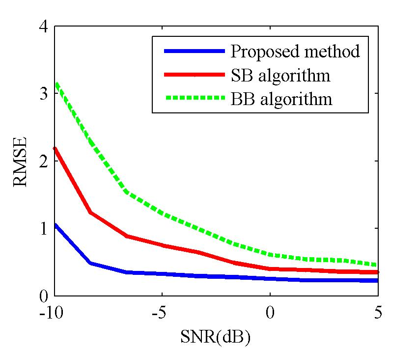
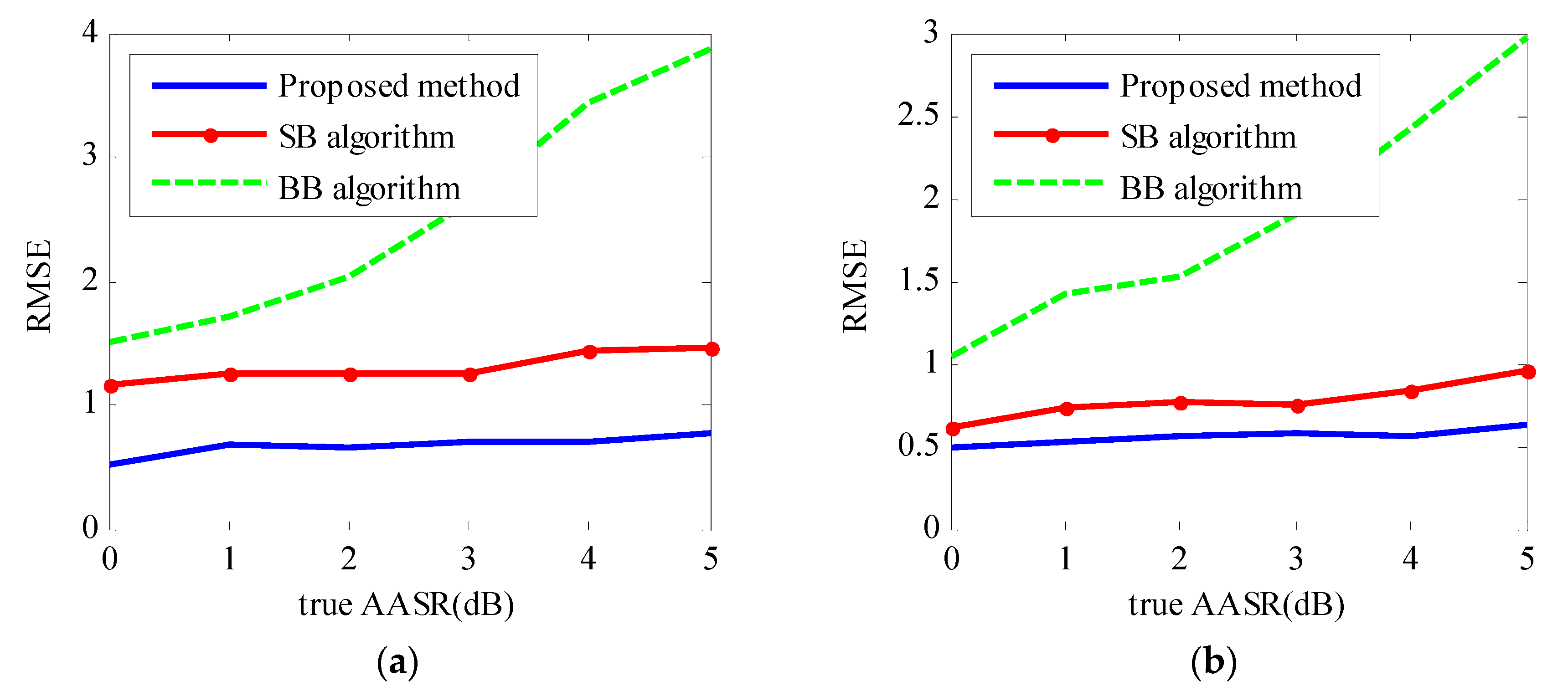
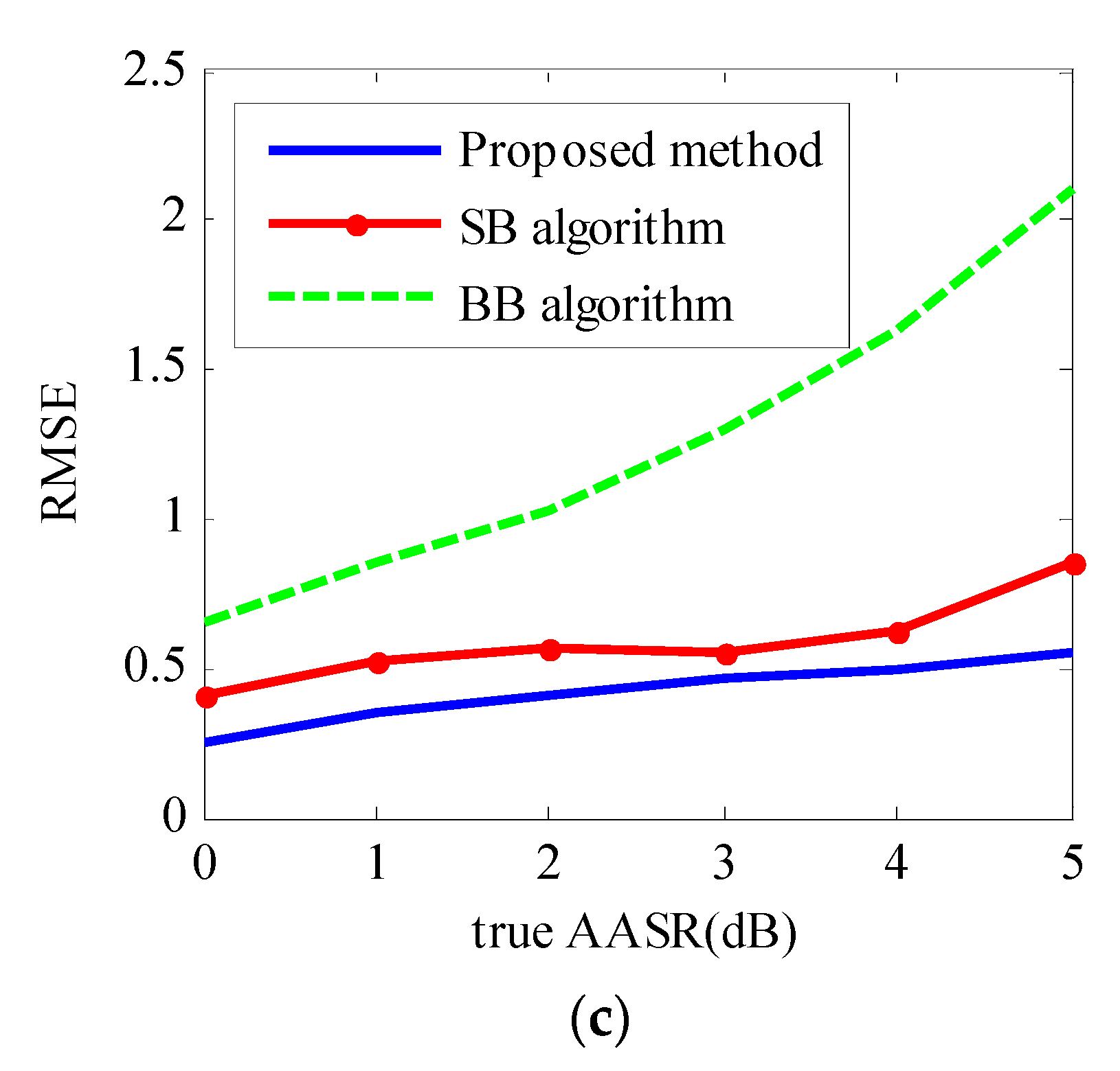
3.3. Comparison of Three Local AASR Estimation Methods

The estimation error of local AASR under different SNR conditions among the proposed methods, BB algorithm, and SB algorithm are simulated in this section. According to the simulation parameters in Table 1, a point target image with a size of 1280 * 1280 is simulated. Point targets are simulated at the position of the main target and the fuzzy targets in the image respectively, and then its AASR is estimated by three algorithms respectively.
Among them, the BB algorithm mainly obtains the ratio of the energy of the blurred position signal to that of the uniform background signal by sufficiently averaging the image of the SAR time domain. According to the literature [13], the simulation process of the SB algorithm is shown in Figure 5, and the left and right AASRs can be obtained by Equation (12).
( A A S R L S B [ x 0 , y 0 ] A A S R R S B [ x 0 , y 0 ] ) = ( P E 1 P E c a L 1 P E 1 P E c a R 1 P E 2 P E c a L 2 P E 2 P E c a R 2 ) 1 ( c m 1 P E 1 P E c m 2 P E 2 P E )
where, c a L 1 , c a L 2 , c a R 1 , c a R 2 , c m 1 and c m 2 can be derived from the literature [13].
Two hundred Monte Carlo random experiments were also performed on the simulation process of the three algorithms. The three curves of Figure 6 are the RMSE of the estimated results of the three algorithms as a function of SNR, respectively.
As can be seen from Figure 6, when the SNR is high, the RMSE of the proposed method is close to the estimation results of the two traditional algorithms. However, when SNR is low, the RMSE of the proposed method is significantly lower than the two traditional local AASR estimation algorithms.
In order to further compare the estimation error of the three algorithms in different AASR values, the RMSE of the estimation results of the three algorithms are simulated when SNR is −5 dB, 0 dB and 5 dB, respectively. The simulation results are shown in Figure 7.
As can be seen from Figure 7, when SNR is low, the estimation results of the proposed method are significantly better than the two traditional estimation algorithms with the increase of AASR. In the case of high SNR, when the AASR is low, the estimation results of the three algorithms are highly consistent; When the AASR is high, the estimation results of this algorithm and the SB algorithm are consistent, which are better than BB algorithm.

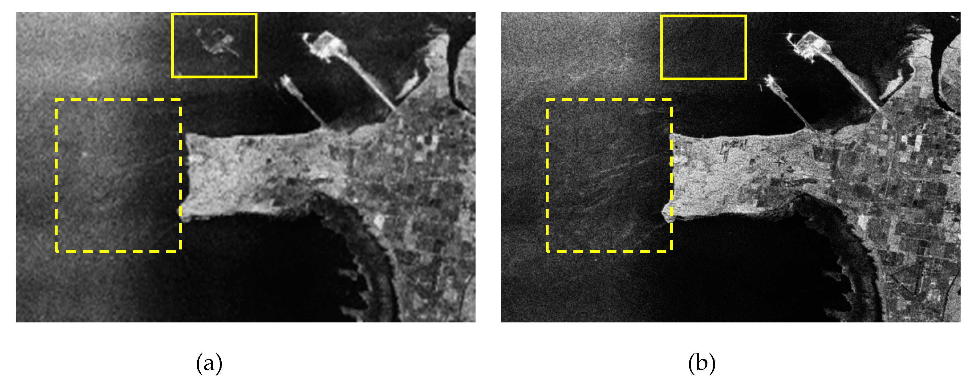
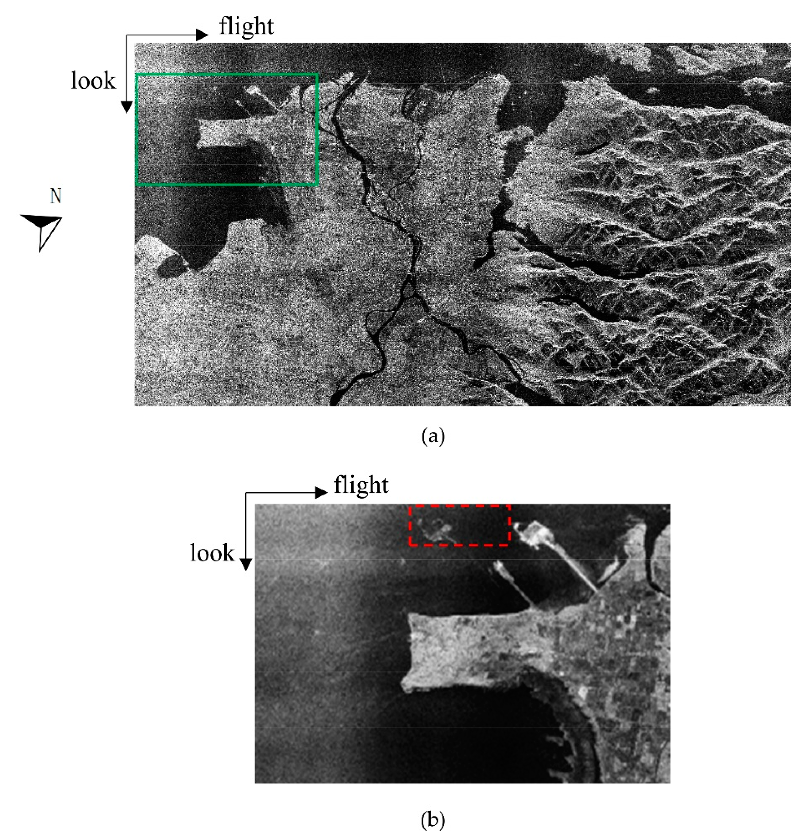
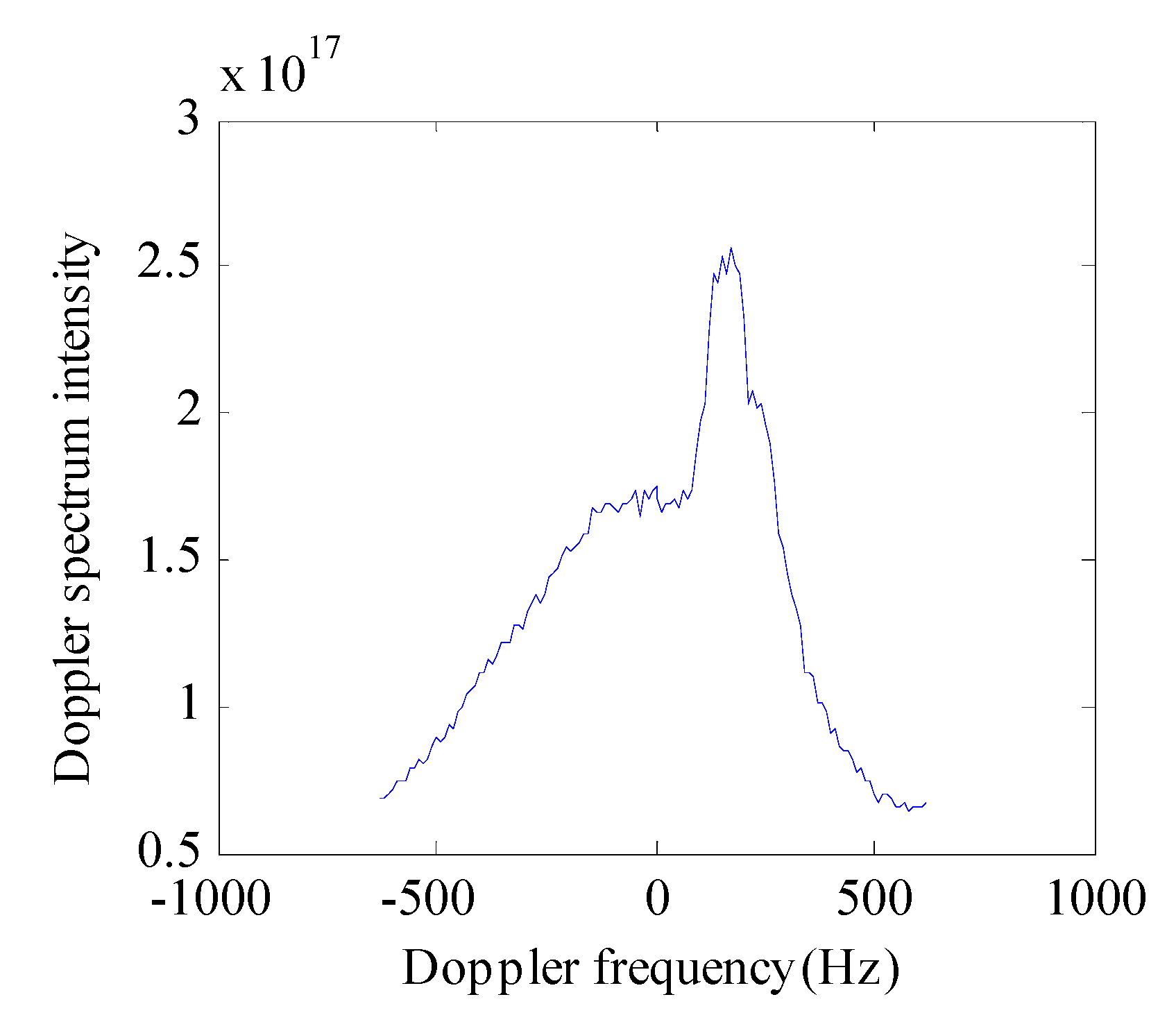
4. Experimental Verification Based on Radarsat-1 Image

In this section, the Radarsat-1 satellite SAR image will be used to verify the proposed method. Its SAR raw data was obtained from the accompanying CD of literature [25]. According to Figure 1, the raw data is first subjected to SAR imaging processing, and the Doppler center frequency is shifted to the zero-frequency position. The imaging process is shown in Figure 8.
SAR imaging results are shown in Figure 9a, Figure 9a is a RADARSAT-1 image of Vancouver. As can be seen from the figure, this SAR image has strong azimuth ambiguity.
As can be seen from Figure 9b, the image area is disturbed by the azimuth ambiguity signal, and the sea surface texture is almost covered by the ambiguity signal. According to the description in the literature [25], the SNR of the water area of this image is −10 dB, the SNR of the land area is 8 dB, and its AASR is about −17 dB. There are clear blur targets in the red dotted frame of Figure 9; therefore, the red dotted frame image in Figure 9 is selected to verify the AASR estimation method.
In the red dotted frame image in Figure 9, there are 1664 pixels in the flight direction, 600 pixels in the look direction, and its SNR is −3.5 dB. In this example, each Doppler spectrum is a 128-point discrete spectrum that is averaged by 13 times in the flight direction and 10 times in the look direction. A total of 60 Doppler spectra from the entire SAR image are obtained. One of the Doppler power spectra obtained is shown in Figure 10.
As can be seen from Figure 10, the Doppler center frequency of the selected image block area has been moved to the zero frequency, and the right edge spectrum of the Doppler spectrum is significantly higher than the left edge spectrum. This is because the left ambiguity caused by the littoral zones is more serious in Figure 9b. Then, according to the theoretical analysis in Section 2, the linear relationship statistics are performed on the Doppler spectrum, and the statistical results are shown in Figure 11.
As can be seen from Figure 11, the Doppler power spectrum in Figure 10 is asymmetrical due to the presence of azimuth ambiguity. However, the points in Figure 11a,b are still evenly distributed on both sides of the fitted curve. According to the estimation theory in Section 2, NAASRl and NAASRr are estimated respectively. Then, the estimation result is substituted into Equation (4), and the final AASR of the image block is obtained. This section also compares the BB algorithm and the SB algorithm with the proposed method. The comparison results are shown in Table 3.
As can be seen from Table 3, the local AASR estimation result of the proposed method is closer to the value of the SB algorithm than that of the BB algorithm. The SB algorithm and the BB algorithm have been compared in [13], both of which have higher estimation results in special conditions. However, the above two algorithms have limitations. The proposed method overcomes their limitations and can accurately estimate the local AASR of SAR images.

5. Discussion

5.1. Applicability Analysis of the Proposed Method

Compared with the traditional AASR estimation algorithms (BB algorithm and SB algorithm), both advantages and disadvantages of the proposed method exist.
The advantages include the following:
(1)
Even in the case of low SNR, the proposed method still has higher estimation accuracy than the traditional AASR estimation algorithms;
(2)
The proposed method starts from the original data and can retain the original information of the echo signal to the maximum extent;
(3)
The fuzzy source signal does not have to appear in the SAR image.
The shortcomings include the following:
(1)
Since AAP must be known, it is necessary to start from the raw data when performing AASR estimation.
(2)
The number of pixels used to calculate the azimuth Doppler power spectrum is large. Therefore, the local AASR resolution of the proposed method is low.
Therefore, this section mainly analyzes the above two shortcomings.

5.1.1. Limitation of Data Selection

The azimuthal resolution of the SAR raw signal is too coarse for most applications. To increase the azimuthal resolution, the azimuthal matching filter must be applied on the SAR raw signal to convert it to a single-look complex image. Therefore, the unweighted azimuthal matching filter can be used, which only changes the phase of the Doppler spectrum without modifying the amplitude of the Doppler spectrum. Thus, the azimuthal power spectrum of the single-look complex image has the same shape characteristic as that of the SAR raw signal. The relationship between the power spectra of the single-look complex images and the SAR raw signal is given as the following:
p s ( f , x 0 , y 0 ) = p r ( f , x 0 , y 0 ) | H ( f ) | 2 = p r ( f , x 0 , y 0 )
where H ( f ) = exp ( j π λ R f 2 2 V 2 ) is the unweighted azimuthal matching filter, p s ( f , x 0 , y 0 ) and p r ( f , x 0 , y 0 ) are the azimuthal power spectra of the single-look complex image and the SAR raw signal, respectively.
This technical requirement undoubtedly limits the scope of application of the proposed method. For SAR products after the second level, if the weighted AAP is known, the proposed method can also be used for AASR estimation. However, in most cases, it is difficult to obtain a weighted AAP. Therefore, the proposed method in this paper is mainly applicable to estimate the AASR from the SAR raw data.

5.1.2. Estimated Resolution of AASR

In this section, according to Table 1, the estimation accuracy of the proposed method is verified by changing the number of pixels used to calculate the Doppler spectrum. The result is shown in Figure 12.
As can be seen from Figure 12, as the number of pixels used to calculate the Doppler power spectrum increases, the RMSE of the estimation result decreases. When RMSE = 0.41, the number of pixels used to calculate the Doppler power spectrum is 1280. This is consistent with the number of azimuth pixels of the point target image generated in the simulation experiment in Section 3.3. In Figure 6, when SNR is 5 dB, AASR is −9.435 dB, the RMSEs of AASR for the proposed method, SB algorithm, and BB algorithm are 0.41, 0.4508, and 0.5302, respectively. According to the literature [13], the AASR estimation resolution of the SB algorithm and the BB algorithm can reach 25 * 25 pixels. However, currently, it is difficult to achieve such high resolution using the proposed method.
In addition, it can be concluded that when the SNR is high, even if the number of pixels used to calculate the Doppler power spectrum is small, the proposed method can also have a high estimation accuracy. When the SNR is low, the number of pixels used to calculate the Doppler power spectrum must be increased to achieve the deserved estimation accuracy.

5.2. Sensitivity Analysis of AAP on AASR Estimation Results

The proposed method in this paper requires a known AAP. Therefore, if the AAP model does not match the real AAP, the estimation result will be inaccurate. The sensitivity of AAP is analyzed by simulations, the results are shown in Figure 2. Where b is the AAP shape factor.
As can be seen from Figure 13, True values are the red lines. When 1381 H z b 1404 H z , the estimated results of the N A A S R l and N A A S R r are close to the true values, and the estimated results of the AASR are also close to the true values. Therefore, we can ascertain that the estimation results of the proposed method are more accurate in this case.

5.3. The Application of the Estimated Local AASR

According to the experimental verification results in Section 4, the AASR in Figure 9b estimated by the proposed method, SB algorithm and BB algorithm are very close. Therefore, this paper mainly uses the AASR estimated by the proposed method to perform azimuth ambiguity suppression.
In order to achieve the effect of suppressing the azimuth ambiguity, according to the and estimated by the proposed method we improve the azimuth filter mentioned in the literature [8], as shown in the following equation:
H f = ( P a ( f ) + N A A S R l | P a ( f F a ) | 2 | P a ( f ) | 2 + N A A S R r | P a ( f + F a ) | 2 | P a ( f ) | 2 + S N R 1 ) 1
The improved azimuth ambiguity suppression process is as follows. Firstly, the SAR raw data in Figure 7b is divided into several sub-blocks, and the AASR of each sub-block is estimated by the proposed method. Secondly, the local Doppler spectrum is weighted by Equation (14). Finally, the SAR data is transformed into the time domain to complete the suppression of azimuth ambiguity. The results are shown in Figure 14.
As can be seen from the position of the solid yellow frame in Figure 14, the improved filter using the proposed method suppresses the azimuth ambiguity signal very well. Moreover, as can be seen from the yellow dotted frame in the figure, the SAR image processed by the proposed method can preserve the original ocean texture while suppressing the azimuth ambiguity. This further illustrates the feasibility and accuracy of the proposed method.

6. Conclusions

In order to solve the problem of the influence of azimuth ambiguity signal on SAR image quality, a local AASR estimation method based on the Doppler power spectrum in SAR images is proposed. The azimuth weighting filter is optimized by estimating the local AASR, thereby achieving the suppression of the azimuth ambiguity.
In order to fully illustrate its feasibility and accuracy, the proposed method is validated by simulation experiments and real spaceborne SAR data experiments. The simulation results show that the local AASR estimated by the proposed method is very close to the true value. In addition, the estimation accuracy of the three algorithms under different SNR conditions is compared and analyzed. In the case of high SNR, the estimation results of proposed method are very consistent with the traditional BB algorithm and SB algorithm. In the case of low SNR, the estimation error of this method is slightly smaller than the traditional two estimation algorithms. In addition, the three estimation methods are compared and verified by the real SAR data of Radarsat-1. The results show that the estimated values of the three estimation methods are close.
The proposed method can estimate the local AASR of SAR images accurately. The disadvantage is that the local AASR resolution estimated by this method is low. Therefore, further research is needed on how to improve the resolution of the estimation result of the local AASR.

Author Contributions

H.M. conceived and performed the experiments; H.M. and J.C. supervised and designed the research and contributed to the article’s organization; Y.W. and Y.L. provided the data for comparative analysis. H.M. and Z.Y. drafted the manuscript, which was revised by all authors. All authors read and approved the final manuscript.

Funding

This research received no external funding.

Acknowledgments

Thanks to the experimental data and financial support provided by the National Key Lab of Microwave Imaging Technology.

Conflicts of Interest

The authors declare no conflict of interest.

References

  1. Chen, J.; Iqbal, M.; Yang, W.; Wang, P.B.; Sun, B. Mitigation of azimuth ambiguities in spaceborne stripmap sar images using selective restoration. IEEE Trans. Geosci. Remote Sens. 2014, 52, 4038–4045. [Google Scholar] [CrossRef]
  2. Li, F.K.; Johnson, W.T.K. Ambiguities in spaceborne synthetic aperture radar systems. IEEE Trans. Aerosp. Electron. Syst. 1983, AES-19, 389–397. [Google Scholar] [CrossRef]
  3. Tomiyasu, K. Tutorial review of synthetic-aperture radar (sar) with applications to imaging of the ocean surface. Proc. IEEE 1978, 66, 563–583. [Google Scholar] [CrossRef]
  4. Moreira, A. Suppressing the azimuth ambiguities in synthetic aperture radar images. IEEE Trans. Geosci. Remote Sens. 1993, 31, 885–895. [Google Scholar] [CrossRef]
  5. Martino, G.D.; Iodice, A.; Riccio, D.; Ruello, G. Filtering of azimuth ambiguity in stripmap synthetic aperture radar images. IEEE J. Sel. Top. Appl. Earth Obs. Remote Sens. 2014, 7, 3967–3978. [Google Scholar] [CrossRef]
  6. Marino, A.; Sanjuan-Ferrer, M.J.; Hajnsek, I.; Ouchi, K. Ship detection with spectral analysis of synthetic aperture radar: A comparison of new and well-known algorithms. Remote Sens. 2015, 7, 5416–5439. [Google Scholar] [CrossRef]
  7. Barbarossa, S.; Levrini, G. An antenna pattern synthesis technique for spaceborne sar performance optimization. IEEE Trans. Geosci. Remote Sens. 1991, 29, 254–259. [Google Scholar] [CrossRef]
  8. Guarnieri, A.M. Adaptive removal of azimuth ambiguities in sar images. IEEE Trans. Geosci. Remote Sens. 2005, 43, 625–633. [Google Scholar] [CrossRef]
  9. Wu, Y.; Yu, Z.; Xiao, P.; Li, C. Suppression of azimuth ambiguities in spaceborne sar images using spectral selection and extrapolation. IEEE Trans. Geosci. Remote Sens. 2018, 56, 1–14. [Google Scholar] [CrossRef]
  10. Wang, W.; Wang, R.; Deng, Y.; Xu, W.; Guo, L.; Hou, L. Azimuth ambiguity suppression with an improved reconstruction method based on antenna pattern for multichannel synthetic aperture radar systems. IET Radarsonar Navig. 2015, 9, 492–500. [Google Scholar] [CrossRef]
  11. Zhang, Z.; Wang, Z.S. On suppressing azimuth Ambiguities of Synthetic aperture radar by three filters. In Proceedings of the 2001 CIE International Conference on Radar Proceedings (Cat No.01TH8559), Beijing, China, 15–18 October 2001; pp. 624–626. [Google Scholar]
  12. Moreira, A.; Misra, T. On the use of the ideal filter concept for improving sar image quality. J. Electromagn. Waves Appl. 1995, 9, 407–420. [Google Scholar]
  13. Villano, M.; Krieger, G. Spectral-based estimation of the local azimuth ambiguity-to-signal ratio in sar images. IEEE Trans. Geosci. Remote Sens. 2014, 52, 2304–2313. [Google Scholar] [CrossRef]
  14. Wei, Z. Synthetic Aperture Radar Satellite; Science Press: Beijing, China, 2001. [Google Scholar]
  15. Massonnet, D.; Souyris, J.-C. Imaging with Synthetic Aperture Radar; CRC Press: Boca Raton, FL, USA, 2008. [Google Scholar]
  16. Meng, H.; Wang, X.; Chong, J.; Wei, X.; Kong, W. Doppler spectrum-based nrcs estimation method for low-scattering areas in ocean sar images. Remote Sens. 2017, 9, 219. [Google Scholar] [CrossRef]
  17. Meng, H.; Wang, X.; Chong, J. An azimuth antenna pattern estimation method based on doppler spectrum in sar ocean images. Sensors 2018, 18, 1081. [Google Scholar] [CrossRef]
  18. Leng, X.; Ji, K.; Zhou, S.; Zou, H. Azimuth ambiguities removal in littoral zones based on multi-temporal sar images. Remote Sens. 2017, 9, 886. [Google Scholar]
  19. Liu, M.; Li, Z.; Liu, B. Spaceborne sar azimuth ambiguities removal based on apodization algorithm. In Proceedings of the 2016 IEEE International Geoscience and Remote Sensing Symposium (IGARSS), Beijing, China, 10–15 July 2016; pp. 1003–1006. [Google Scholar]
  20. Hawkins, R.K.; Teany, L.D.; Srivastava, S.; Tam, S.Y.K. Radarsat precision transponder. Adv. Space Res. 1997, 19, 1455–1465. [Google Scholar] [CrossRef]
  21. Jackson, H.; Sinclair, I.; Tam, S. Envisat/asar precision transponders. Eur. Space Agency-Publ. -Esa Sp 2000, 450, 311–316. [Google Scholar]
  22. Bamler, R. Doppler frequency estimation and the cramer-rao bound. IEEE Trans. Geosci. Remote Sens. 1991, 29, 385–390. [Google Scholar] [CrossRef]
  23. Madsen, S.N. Estimating the doppler centroid of sar data. IEEE Trans. Aerosp. Electron. Syst. 1989, 25, 134–140. [Google Scholar] [CrossRef]
  24. Chang, C.-Y.; Curlander, J.C. Application of the multiple prf technique to resolve doppler centroid estimation ambiguity for spaceborne sar. IEEE Trans. Geosci. Remote Sens. 1992, 30, 941–949. [Google Scholar] [CrossRef]
  25. Cumming, I.G.; Wong, F.H. Digital processing of synthetic aperture radar data. Artech House 2005, 1, 3. [Google Scholar]
Figure 1. The flow chart of the proposed method. SAR: synthetic aperture radar; AASR: azimuth ambiguity-to-signal ratio.
Remotesensing 11 00857 g001
Figure 2. Simulated Doppler spectrum. (a) Before multi-looking; (b) After multi-looking.
Remotesensing 11 00857 g002
Figure 3. Relationship between P ( 0 ) P ( F a / 2 ) , P ( 0 ) P ( F a / 2 ) and P ( 0 ) for the simulated data. (a) Relationship between P ( 0 ) P ( F a / 2 ) and P ( 0 ) ; (b) Relationship between P ( 0 ) P ( F a / 2 ) and P ( 0 ) .
Remotesensing 11 00857 g003
Figure 4. The root mean squared error (RMSE) of the azimuth ambiguity estimation results as a function of the signal-to-noise ratio (SNR). (a) The RMSE of the left ambiguity estimation result changes with SNR; (b) The RMSE of the right ambiguity estimation result changes with SNR.
Remotesensing 11 00857 g004
Figure 5. The flow chart of spectral-based (SB) algorithm [13].
Remotesensing 11 00857 g005
Figure 6. The comparison results of the RMSE of the three local AASR estimation algorithms (The proposed method, BB algorithm, and SB algorithm using H k ( f y ) with P a L / P m = 1 [13]). Where, Local A A S R = 20.53   d B .
Remotesensing 11 00857 g006
Figure 7. The comparison results of the RMSE of three AASR estimation algorithms under different AASR true values. (a) SNR = 5 dB ; (b) SNR = 0 dB ; (c) SNR = 5 dB .
Remotesensing 11 00857 g007aRemotesensing 11 00857 g007b
Figure 8. SAR imaging process.
Remotesensing 11 00857 g008
Figure 9. Radarsat-1 SAR image of Vancouver collected on 16 June 2002, at 02:24 UTC. (a) Full image; (b) An enlarged view of the green box in Figure 9a.
Remotesensing 11 00857 g009
Figure 10. The Doppler power spectrum of the selected image block.
Remotesensing 11 00857 g010
Figure 11. The relationship between P ( 0 ) P ( F a / 2 ) , P ( 0 ) P ( F a / 2 ) and P ( 0 ) in Figure 10. (a) The relationship between P ( 0 ) P ( F a / 2 ) and P ( 0 ) ; (b) The relationship between P ( 0 ) P ( F a / 2 ) and P ( 0 ) .
Remotesensing 11 00857 g011
Figure 12. RMSE of the AASR estimation results as a function of pixels used to calculate the Doppler power spectrum.
Remotesensing 11 00857 g012
Figure 13. Sensitivity analysis of AAP on A A S R estimation results. (a) The N A A S R r is a function of b; (b) The N A A S R l is a function of b; (c) The A A S R is a function of b.
Remotesensing 11 00857 g013
Figure 14. Azimuth ambiguity suppression result. (a) The original Figure; (b) The results of ambiguity suppression using the AASR estimated by the proposed method.
Remotesensing 11 00857 g014
Table 1. Parameters of the simulated data.
Parametric NameParametric SymbolParametric Value
Number of Doppler spectrum pixels L 128
Pulse repetition frequency (Hz) F a 1256.98
Simulation repeat number R e p e a t _ n u m b e r 800
Look number of SAR image M 10
Signal-to-Noise Ratio (dB) S N R 5
Platform Velocity (m/s) V 7062
Antenna Length (m) L a 10
Wavelength (m)——0.0566
Sampling bandwidth (Hz)—— 32.317 × 10 6
AAP scale factor (Hz) b 1.1 × F a
Ratio of the NRCS values of the left ambiguity signal and the real target position N A A S R l 1
Ratio of the NRCS values of the right ambiguity signal and the real target position N A A S R r 2
Table 2. Comparison of simulation results.
ParametersTrue ValueEstimated Value
N A A S R l 10.997
N A A S R r 21.9125
A A S R −20.53(dB)−0.94(dB)
Table 3. Comparison of results of three local AASR estimation methods.
Estimation MethodMean of AASR Estimates
BB algorithm−16.01 dB
SB algorithm−16.35 dB
Proposed method−16.57 dB
True value−17 dB

