Integrating Growth and Environmental Parameters to Discriminate Powdery Mildew and Aphid of Winter Wheat Using Bi-Temporal Landsat-8 Imagery

Abstract

Monitoring and discriminating co-epidemic diseases and pests at regional scales are of practical importance in guiding differential treatment. A combination of vegetation and environmental parameters could improve the accuracy for discriminating crop diseases and pests. Different diseases and pests could cause similar stresses and symptoms during the same crop growth period, so combining growth period information can be useful for discerning different changes in crop diseases and pests. Additionally, problems associated with imbalanced data often have detrimental effects on the performance of image classification. In this study, we developed an approach for discriminating crop diseases and pests based on bi-temporal Landsat-8 satellite imagery integrating both crop growth and environmental parameters. As a case study, the approach was applied to data during a period of typical co-epidemic outbreak of winter wheat powdery mildew and aphids in the Shijiazhuang area of Hebei Province, China. Firstly, bi-temporal remotely sensed features characterizing growth indices and environmental factors were calculated based on two Landsat-8 images. The synthetic minority oversampling technique (SMOTE) algorithm was used to resample the imbalanced training data set before model construction. Then, a back propagation neural network (BPNN) based on a new training data set balanced by the SMOTE approach (SMOTE-BPNN) was developed to generate the regional wheat disease and pest distribution maps. The original training data set-based BPNN and support vector machine (SVM) methods were used for comparison and testing of the initial results. Our findings suggest that the proposed approach incorporating both growth and environmental parameters of different crop periods could distinguish wheat powdery mildew and aphids at the regional scale. The bi-temporal growth indices and environmental factors-based SMOTE-BPNN, BPNN, and SVM models all had an overall accuracy high than 80%. Meanwhile, the SMOTE-BPNN method had the highest G-means among the three methods. These results revealed that the combination of bi-temporal crop growth and environmental parameters is essential for improving the accuracy of the crop disease and pest discriminating models. The combination of SMOTE and BPNN could effectively improve the discrimination accuracy of the minor disease or pest.

1. Introduction

Powdery mildew (Blumeria graminis), a crop disease, and aphids (Sitobion avenae), an insect pest, are both destructive and occur almost each year in major winter wheat growing regions in China [1,2]. These two threats can result in a serious loss of grain yield and quality, the annual average occurrence area of powdery mildew was recorded to be as high as 10 million ha during 2000 to 2016, annual aphid damage affects 13 million ha and causes of up to 40% wheat yield loss in China [3,4,5,6,7]. In practice, wheat powdery mildew and aphids tend to occur in fields unpredictably, making real-time characterization, identification, and classification of different diseases and pests very necessary to mitigate the problems associated with disease and pest monitoring and pesticide overuse [8].

Remote sensing technology is an important alternative of traditional manual scouting in crop disease and pest monitoring. Some researchers demonstrated the feasibility of remote sensing technology in detecting and differentiating crop diseases and pests according to hyperspectral analysis. For instance, Feng et al. [9] suggested that the best two-band vegetation index ranges for powdery mildew detection of different incidence levels were between 570–590 nm and 536–566 nm for the ratio index, and 568–592 nm and 528–570 nm for the normalized difference index. Riedell et al. [10] characterized leaf reflectance spectra of wheat damaged by Russian wheat aphids and greenbugs, finding the chlorophyll concentrations of the plants damaged by the two aphids significantly influenced the reflectance in the 625–635 nm and the 680–695 nm ranges. Huang et al. [11] found single wavelengths around 400 nm, 500 nm, and 750 nm were highly relevant for wheat leaves diseased with powdery mildew, single wavelengths around 540 nm and 750 nm were relevant to wheat yellow rust, and single wavelength around 400 nm was relevant to wheat aphid infection. Based on these findings, they developed four new spectral indices and successfully identified healthy leaves and leaves infected with powdery mildew, yellow rust, and aphid using them. In addition, based on an advanced hyperspectral analysis technique, continuous wavelet analysis, Shi et al. [4] determined the most sensitive wavelet features (WFs) for the identification of yellow rust and powdery mildew in winter wheat. Although these hyperspectral based studies gave more detailed information and demonstrated the effectiveness of hyperspectral sensors in detecting and discriminating crop diseases and pests, its high hardware and computational costs restrict its application over large areas [12,13]. Based on the acceptable spatial and temporal resolutions, multispectral satellite technique becomes a feasible method for crop diseases and pests monitoring [8,14,15]. For instance, based on Landsat-5 Thematic Mapper (TM) data, Mirik et al. [16] successfully assessed the infection and progression of wheat streak mosaic. Navrozidis et al. [17] demonstrated that field spectroscopy and wide area remote sensing (i.e., Landsat-8) can be used to create sufficiently accurate quantification models of crop disease severity. Furthermore, relying on a relative spectral response function (RSR function) spectral simulation, Yuan et al. [12] converted canopy hyperspectral signals to broadband reflectance corresponding to seven high-resolution satellite sensors and channel settings, and simulated some classic vegetation indices to discriminate three typical diseases and an insect pest of winter wheat, and their results indicated the feasibility of high resolution multispectral satellite sensors for discriminating crop diseases and pests. By developing a set of normalized bi-temporal vegetation indices using PlanetScope image datasets at a 3-m spatial resolution, Shi et al. [8] mapped and evaluated the damage caused by rice dwarf, rice blast, and glume blight at fine spatial scales. These results motivate us to attempt to discriminate wheat powdery mildew and aphid using multispectral satellite imagery.

For one thing, different diseases and pests could cause similar stresses and symptoms such as discoloration, wilting, and rot. For another, in different growth periods, the occurrence and epidemic law of different diseases and pests are different. Both of which may result in confusion for multiple damage detection using a single-date satellite imagery. The information gathered on within-field variability in growth conditions and diseases and pest infestations is important for precision crop diseases and pests monitoring through multi-temporal remote sensing imagery [8,14,18]. Furthermore, the occurrence and development of crop diseases and pests not only are related to crop growth conditions, but also require appropriate environmental conditions such as temperature, humidity, etc. [19]. The monitoring accuracy of crop diseases and pests could be improved by integrating environmental information [3,19]. The effectiveness of field environmental parameters such as land surface temperature (LST), soil water content (SWC) and the tasseled cap transformation features (Greenness and Wetness) based on remotely-sensed shortwave infrared and thermal infrared information of Landsat-8 imagery for crop disease and pest monitoring have been demonstrated [3,19,20]. However, most existing models for monitoring crop diseases and pests by remote sensing focus on detection and monitoring of crop damages using corresponding single-date imagery; meanwhile, crop environmental characteristics have not been considered [13,20,21,22]. Some other scholars only considered either temporal information or crop environment in disease and pest monitoring instead of both factors, few studies combined the information from these two aspects into disease and pest monitoring and differentiation [8,19]. Therefore, it is necessary to evaluate the feasibility of remotely sensed feature set integrating multi-temporal crop growth indices and environmental factors in monitoring and discriminating crop diseases and pests.

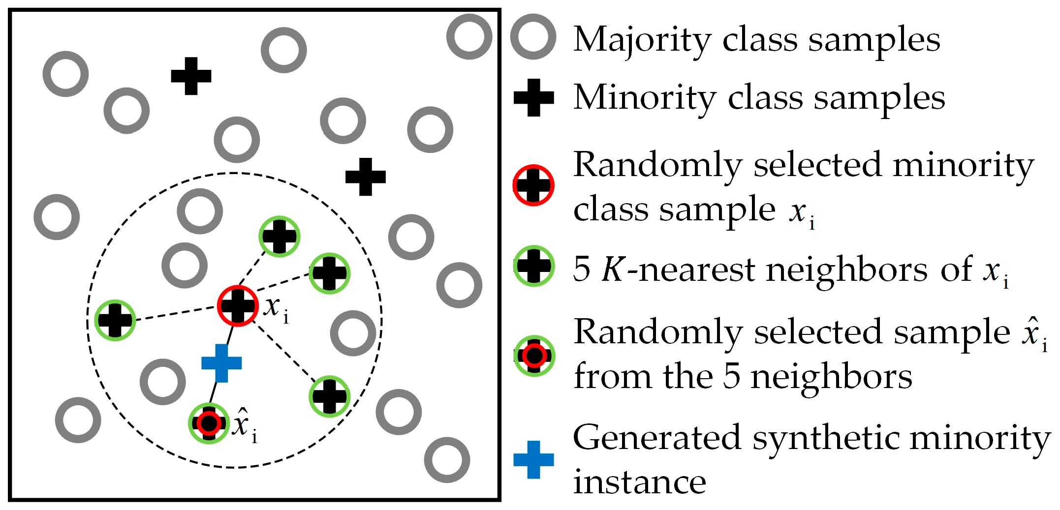
There is often a situation in the field where one crop stress is dominant and other stresses are mild but important. An imbalanced data set is formed if one class has a significantly different number of samples from other classes for a field survey experiment. For an imbalanced data set, more attention needs to be paid to the minority class that contains more valuable information [23]. However, when samples of the majority class in a training data set vastly outnumber those of the minority class, traditional data mining algorithms tend to ignore the minority class because of the pursuit of global accuracy [24,25]. The synthetic minority oversampling technique (SMOTE) proposed by Chawla et al. [26] was a popular method through oversampling at the connection between the current samples of the minority class to get synthetic samples of the minority class to balance the proportions in classes. This method was widely used in combination with a variety of traditional classification methods to solve the classification problem of imbalanced data [27,28].

Back propagation neural network (BPNN) is a popular classification method for its back propagation-learning algorithm, which is a mentor-learning algorithm of gradient descent, or its alteration [29]. BPNN is a multilayer mapping network that minimizes an error backward while information is transmitted forward [30]. The BPNN method can implement any complex nonlinear mapping function proven by mathematical theories and approximate any arbitrary nonlinear function with satisfactory precision, which makes BPNN popular for predicting complex nonlinear systems [31,32]. The BPNN method has some advantages such as simple architecture, easy model construction and rapid calculation speed [33]. The BPNN method has been widely used for classification [33,34,35,36,37]. These existing successful cases support the use of BPNN in this study for the discrimination of wheat powdery mildew and aphid.

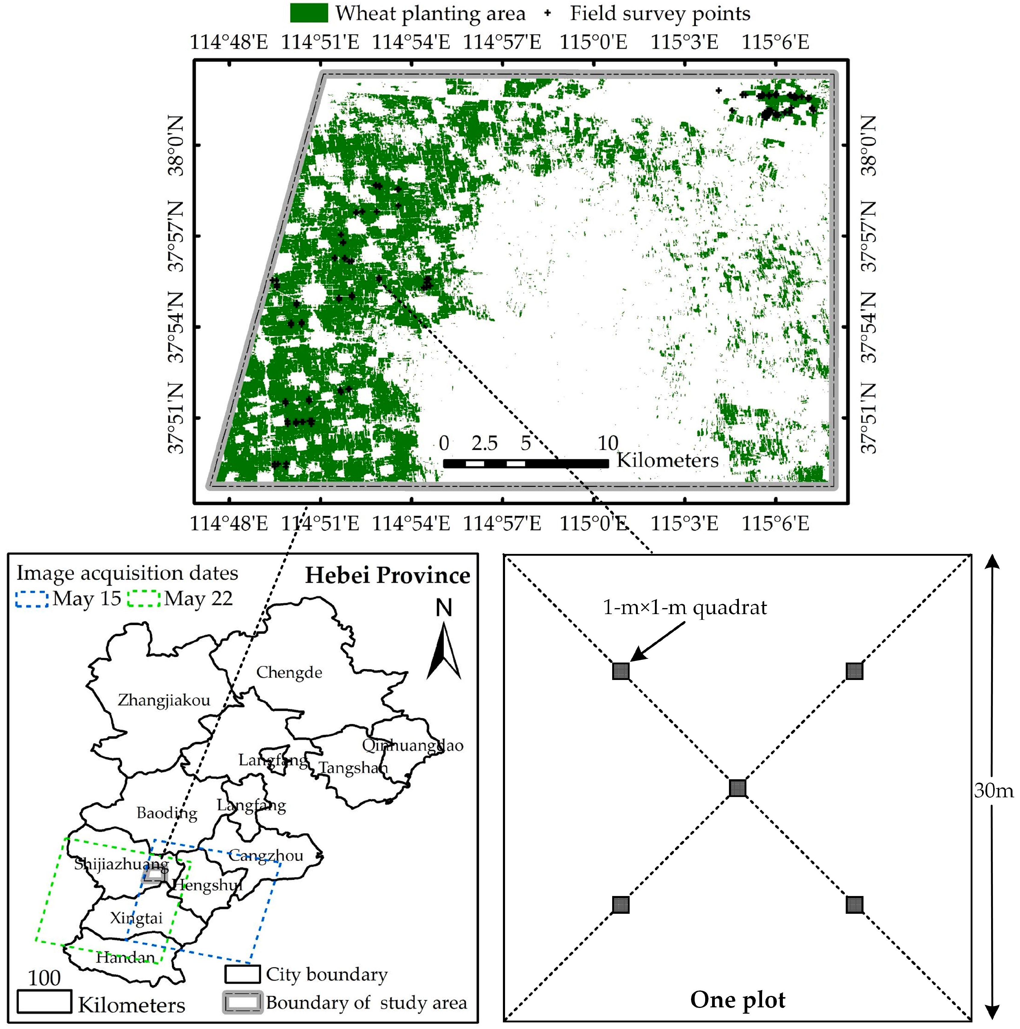
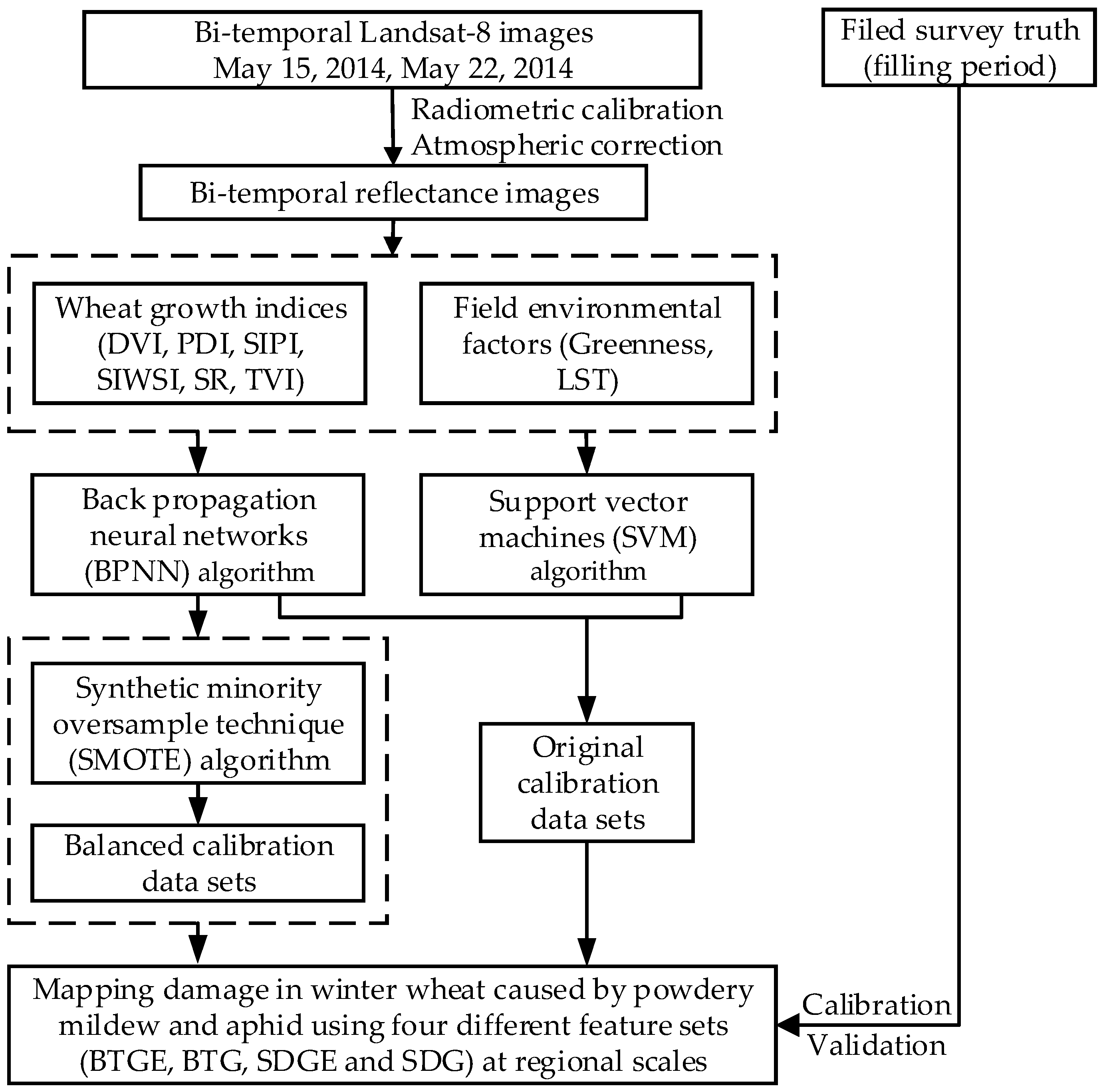
In this study, a coupled SMOTE-BPNN model integrating bi-temporal growth indices and environmental factors has been developed, which can accurately discriminate different damages in winter wheat. The simultaneous outbreak of wheat powdery mildew and wheat aphid was chosen for the case study. Wheat powdery mildew and aphid occurred in the Shijiazhuang area of Hebei Province, China, during the spring of 2014. Bi-temporal Landsat-8 imagery was used in this study. Both wheat growth and environmental parameters were used in combination. The aims of this study were: (1) to evaluate the performance of the coupled SMOTE-BPNN classification models for mapping the damage from the disease and pest; and (2) to assess the impact of the feature set consisting of bi-temporal growth indices and environmental factors on the accuracy of the classification models when it is considered as an input parameter.

2. Materials and Methods

2.1. Study Site

The study site was located in the Shijiazhuang area of Hebei Province, in the northern part of the North China Plain (Figure 1). This region has a warm temperate humid or semi-humid climate, with four distinctive seasons. The average annual temperature ranges from 12 to 13 °C, and the annual precipitation ranges 400 to 800 mm [38]. The annual frost-free period ranges 175 to 220 days. Winter wheat is usually planted in early October and harvested in the middle of June [39]. The major soil type in this region is reported to be Haplic Luvisols [40]. Suitable temperature and abundant sunshine make it suitable for crop growth. Winter wheat is a major local crop. The local climate and environmental conditions provide a suitable developing environment for powdery mildew and aphid [19]. Due to its single planting pattern, this region is an ideal location for remote sensing monitoring.

2.2. Field Survey

A total of 137 field plots were surveyed to evaluate the damage severity caused by winter wheat powdery mildew and aphid as ground truth data during 23 to 28 May 2014 of the grain filling period, when symptoms of diseases and pests are most visually conspicuous. Five 1-m × 1-m quadrats were selected at a 30-m × 30-m plot to match the spatial resolution of Landsat-8 satellite imagery. The center latitude and longitude of each plot were recorded by a sub-meter precision handheld global positioning system (GPS) receiver. Wheat growth conditions, height, and disease and pest occurrence severity were recorded in the survey (

Table A1. Summary of the field survey indicators.

Type	Field Survey Indicators
Growth conditions	Population density ①	Plant height	Growth period
Powdery mildew ②	Damage percentage	Disease severity	Disease index, DI
Aphid ③	Aphid amount	Aphid density	Aphid severity

Note: Based on the combination scheme of random sampling and representative sampling, each sample plot of 30-m × 30-m was designed to match the spatial resolution of Landsat-8 satellite imagery. At each plot, five 1-m × 1-m quadrats were selected to survey damage severity through diagonal sampling:

• Population density is the total number of plants in one 1-m × 1-m quadrat.
• In each quadrat, 20 individual plants were random selected for damage percentage inspection. In disease inspection, according to the National Rules for the Investigation and Forecasting of Crop Diseases (NY/T 613-2002), each leaf of the selected plants were grouped into one of 10 disease severities: 0 (amount of infection: 0%), 1 (1–10%), 2 (11–20%), 3 (21–30%), 4 (31–40%), 5 (41–50%), 6 (51–60%), 7 (61–70%), 8 (71–80%), and 9 (81–100%). Of them, 0% represents no infection and 100% represents the greatest amount of infection. Then, the disease index (DI) was calculated using following formula:

  $$DI=\frac{{\displaystyle \sum xf}}{n{\displaystyle \sum f}}\times 100,$$

  (4)

  where x is the value of incidence level, f is the total number of leaves for each degree of disease severity, and n is the value of highest disease severity gradient. The DIs of five quadrats within a plot were then averaged to represent the disease severity of the plot:
• In each quadrat, 10 individual plants were random selected for amount inspection. In pest inspection, the aphid densities were then estimated by using following formula: aphid density = total aphid amount/10 plants. The average aphid density of five quadrats was used to represent the aphid density of the plot. According to the Rules for the Investigation and Forecast of Wheat Aphides (NY/T 612-2002), the six aphid damage severities were assessed.

). The sampling designs for wheat powdery mildew and aphid were based on the Rules for the Investigation and Forecast of Wheat Powdery Mildew (NY/T 613-2002) and the Rules for the Investigation and Forecast of Wheat Aphides (NY/T 612-2002). A visual discrimination method was used to assess the infestation status and damage severity for each plot because wheat powdery mildew and aphid occurred simultaneously in some of the plots. The plots were labeled as healthy if they had not been infested or if the proportion of damaged leaves was less than 10%. For a total of 137 plots, 46 plots were healthy, 80 plots were infected by powdery mildew, and 11 plots were damaged by aphid. In this study, 91 plots were randomly selected for model training and the remaining 46 plots were used for testing.

Table 1. Basic information for the disease survey experiment.

Type	Number of Field Survey Samples
	Healthy	Powdery Mildew Infected	Aphid Damaged
Training	30	54	7
Testing	16	26	4

lists the overview of the field survey experiment.

2.3. Image Selection and Preprocessing

Considering the potential pathological impact of disease and pest infestations, multi-temporal remote sensing imagery could monitor and discriminate crop diseases and pests more accurately [14]. Therefore, according to wheat powdery mildew and aphid occurrence and development characteristics [41,42,43], two Landsat 8 satellite scenes acquired on 15 and 22 May 2014 were selected in this study. Due to the special location of the study area, which located the overlapping area of the two images, the two scenes were with a time interval of less than 16 days. Both images covered the entire study area without any cloud. A radiometric calibration and an atmospheric correction for the images were performed using ENVI 5.3 software (Harris Geospatial Solutions, USA). In addition, a decision tree method was applied to the extraction of the winter wheat planting area based on the different time distribution characteristics of the main crops (mainly include wheat, corn and cotton) in the study area [44,45,46]. An overall validation accuracy of 94% through field survey points were obtained, and the result satisfied the accuracy requirement for subsequent analysis.

2.4. Extraction of Crop Growth Characteristics and Field Environmental Parameters

The occurrence of powdery mildew and aphid is not only determined by crop growth conditions, but also strongly related to environmental factors (i.e., temperature and humidity). Therefore, in this study, six spectral indices related to crop growth and two environmental factors were extracted and calculated to investigate their sensitivity for the discrimination of winter wheat powdery mildew and aphid. The six spectral indices include: difference vegetation index (DVI), perpendicular drought index (PDI), structural independent pigment index (SIPI), shortwave infrared water stress index (SIWSI), simple ratio index (SR), and triangular vegetation index (TVI). These indices are respectively related to vegetation coverage, drought condition, senescence, canopy water content, photosynthetic area and radiant absorption of chlorophyll. The formulas for these indices are provided in

Table 2. Summary of the remotely sensed features used for discrimination of powdery mildew and aphid, with red band, green band, near infrared (NIR) band, and short wave infrared (SWIR) band denoted as R_R, R_G, R_NIR, and R_SWIR, respectively.

Category	Definition	Formula or Description	Sensitive to	Reference
Crop growth characteristics	Difference vegetation index, DVI	$R_{NIR}-R_R$	Vegetation coverage	[48]
	Perpendicular drought index, PDI	$\left(1/\mathrm{sqrt}\left(M^2+1\right)\right)\left(R_R+M{R}_{NIR}\right)$	Drought condition	[49]
	Structural independent pigment index, SIPI	$\left(R_{NIR}-R_B\right)/\left(R_{NIR}-R_R\right)$	Senescence	[50]
	Shortwave infrared water stress index, SIWSI	$\left(R_{NIR}-R_{SWIR}\right)/\left(R_{NIR}+R_{SWIR}\right)$	Canopy water content	[51]
	Simple ratio index, SR	$R_{NIR}/R_R$	Photosynthetic area	[52]
	Triangular vegetation index, TVI	$60\left(R_{NIR}-R_G\right)-100\left(R_R-R_G\right)$	Radiant absorption of chlorophyll	[53]
Field environmental parameters	Greenness	A tasseled cap transformation feature	Overall crop growth	[47]
	Land surface temperature, LST	Calculated by the single channel method based on the TIRS-1 band of Landsat-8	Crop respiration and transpiration	[54,55]

. The two environmental factors are Greenness and land surface temperature (LST). As a tasseled cap transformation feature, Greenness indicates overall crop growth, and it is also suitable for the characterization of field environmental factors [19]. The Greenness calculation formula [47] is shown in Equation (1):

$$Greenness=g_1\ast b_1+g_2\ast b_2+g_3\ast b_3+g_4\ast b_4+g_5\ast b_5+g_6\ast b_6,$$

(1)

where g_i and b_i (i = 1, 2, …, 6) represent the corresponding coefficient and reflectance for each band (

Table 3. Tasseled cap transformation coefficients of Greenness for Landsat-8 at satellite reflectance.

Index	Bands
Greenness	g1 Blue	g2 Green	g3 Red	g4 NIR	g5 SWIR-1	g6 SWIR-2
	–0.2941	–0.243	–0.5424	0.7276	0.0713	–0.1608

).

LST reflects the intensity of crop respiration and transpiration, and it is also related to the occurrence of crop diseases and pests. The single channel method and the TIRS-1 (tenth band of Landsat-8 imagery) of the thermal infrared sensor was used to calculate LST as shown in Equation (2) [19]:

$$LST=(K_2/\ln (K_1/L_{\lambda }+1))+1,$$

(2)

where L_λ is the spectral radiation rate of the TIRS-1 band, (W/m2*sr*μm); K₁ and K₂ are conversion constants obtained from the heading file of the images (K₁ = 774.89, K₂ = 1321.08).

Finally, a total of 16 remote sensing features (eight features for each period) of the two periods were extracted.

2.5. Balance Training Data Using Synthetic Minority Oversample Technique (SMOTE) Algorithm

Before the construction of crop disease and pest discrimination models, the SMOTE algorithm was firstly used to get synthetic samples of minority classes (both healthy and aphid damaged) to balance the proportions in classes of the training data set in this study. SMOTE uses samples of the minority class to control the generation and distribution of artificial samples to achieve the purpose of balancing datasets [56,57]. It can achieve potentially better classification performance without loss of data [26,58]. SMOTE assumes that a sample constructed between the nearby samples in the minority class is still a sample of the class [56]. In order to avoid the over-fitting problem while expanding the minority class region, SMOTE generates new instances by operating within the existing feature space. New instance values are derived from interpolation rather than extrapolation, so they still carry relevance to the underlying data set [57]. For each minority class instance, SMOTE interpolates values using a K-nearest neighbor technique and creates attribute values for new data instances [59]. Specifically, the basic principles of the SMOTE algorithm is as follows:

• For each sample in the minority class x_i, the K-nearest neighbors belonging to the same class are searched.
• Randomly select one sample ${\widehat{x}}_i$ from the K-nearest neighbors.
• Construct one new artificial minority class sample x_new between the two samples using Equation (3):

  $$x_{new}=x_i+rand[0,1]\times ({\widehat{x}}_i-x_i),$$

  (3)

  where x_new is the new synthetic minority class sample. x_i is the minority class samples, i = 1, …, N, N is the amount of SMOTE determined based on the imbalanced proportion of samples. rand[0, 1] is a random number between 0 and 1. ${\widehat{x}}_i$ is a random K-nearest neighbor sample of the x_i.

Figure 2 gives an example to further illustrate the basic principles of the SMOTE algorithm.

After SMOTE processing, the number of minority class will increase K times. If more artificial minority class samples are needed, the above interpolation process is repeated to achieve a balance in the new training samples and the new sample dataset is finally used for training the classifier. These synthetic samples help to break the drawback of simple up-sampling. The increase of the original dataset in this way can significantly improve the learning capacity of the classifier. SMOTE was used to generate a new balanced training data set for the training of the crop disease and pest discrimination models. Furthermore, the coefficient of determination (R²) was used as accuracy measurement of the new balanced training data set estimation. If the value of R² reaches over than 0.7, the new balanced training data set is considered to be with good quality and suitable for the models construction.

2.6. Wheat Powdery Mildew and Aphid Discriminate Using Back Propagation Neural Networks (BPNN)

The BPNN algorithm was implemented to discriminate wheat powdery mildew and aphid based on the bi-temporal remote sensing feature set which includes both growth indices and environmental factors. BPNN is a method designed to minimize the total error (or mean error) of the output computed by the network [30]. Generally, a network is composed of an input layer, an output layer, and one or more hidden layers between them [60]. Network training is a process of continual readjustment between the weights and the threshold, in order to make the network error reduce to a preset minimum or stop at a preset training step. Then, the forecasting samples are input to the trained network to obtain the forecasting results. It is reported that the improvement of control performance of BPNN algorithm was not proportional to the increased number of hidden layers, and the three-layer (with one single hidden layer) BPNN was the best [61,62]. In addition, the number of hidden neurons in a three-layer network was suggested to be 75% of the number input neurons [63]. Thus, the monolayer structure was adopted for the hidden layer in this study and included twelve neurons. Logsig and purelin were adopted as the activation functions, respectively. One momentum adaptive training function traingdx was utilized by the network training. Based on the classical back propagation algorithm, this algorithm can automatically modulate learning rate and incidental momentum, avoiding local minimum and greatly accelerating the convergence rate greatly [64]. The number of training epochs was used as the stopping criterion in this study, and the allowed maximum epochs were taken as 2000 epochs. Then, a coupled SMOTE-BPNN approach for crop disease and pest discrimination was proposed by combining the new training data balanced by the SMOTE algorithm with the BPNN classification method. All BPNN-related analyses were performed in MATLAB 2016a software.

2.7. Accuracy Assessment of Disease and Pest Discrimination

Overall accuracy (OA), user’s accuracy (UA), producer’s accuracy (PA), and kappa coefficient (

Table 4. Summary of the accuracy measures for discrimination models.

Name	Formula	References
User’s accuracy, UA	$U{A}_i=p_{ii}/p_{i+}$	[70]
Producer’s accuracy, PA	$P{A}_i=p_{ii}/p_{+i}$	[70]
Overall accuracy, OA	$OA={\displaystyle \sum _{i=1}^m{p}_{ii}}/p$	[70]
Kappa coefficient	$kappa=(OA-EA)/(1-EA),EA={\displaystyle \sum _{i=1}^m\frac{p_{i+}}{p}}\frac{p_{+i}}{p}$	[71]

Note: i is the wheat damage category in this study, i = 1, i = 2 and i = 3 mean healthy, powdery mildew infected and aphid damaged, respectively. UA_i, PA_i, and OA mean the user’s accuracy of the category i, the producer’s accuracy of the category i, and the overall accuracy of the classification models, respectively. p_ii, p_i+, p_+i, p mean the correct classification number of the category i, the total number of the category i obtained from the field truth survey, the total number of the category i obtained from the classification models, and the total number of all the three categories, respectively. m is the number of the categories, which equals 3 in this study.

) [65] were calculated for the monitoring results based on field truthing. These accuracy measures were used to evaluate the model’s performance in discriminating crop diseases and pests. To compare and verify the performance of the SMOTE-BPNN models based on bi-temporal growth indices and environmental factors (BTGE), the original training data set-based BPNN and support vector machine (SVM) methods were also used to build discrimination models. To further compare and verify the performance of the bi-temporal feature set-based SMOTE-BPNN discrimination models, the three other feature sets-based models were also constructed using SMOTE-BPNN, BPNN and SVM methods. These feature sets include bi-temporal growth indices (BTG), single-date growth indices and environmental factors (SDGE), and single-date growth indices (SDG). Furthermore, the commonly used parameters F-score and geometric mean (G-means) for imbalanced data sets had also been used to evaluate the proposed models [66,67]. F-score is defined as the harmonic mean of precision and recall, the F-score value increases proportionally to the increase of precision and recall, and a higher F-score value indicates that the model performs better on the minority class samples balancing [66,68,69]. G-means indicates the balance between classification performances on the majority and minority classes [69]. A poor performance in prediction of the minority class examples will lead to a low G-means, even if the majority class examples are correctly classified per the model. G-means is quite important to measure the avoidance of the overfitting to the majority class samples and the degree to which the minority class samples is marginalized [66,69]. F-score was used to measure classification performance of the SMOTE-BPNN approach on rare classes (include healthy and aphid), and G-means was used to measure the classification performance of the whole data set in this study. Figure 3 summarizes the data analysis process.

3. Results

3.1. Response of Remotely Sensed Features to Powdery Mildew and Aphids

The responses of the eight remotely sensed features during the two growth periods to changes in powdery mildew and aphids are illustrated in Figure 4. The features were compared at different damage levels using the mean and standard deviation of each normalized feature. The results reveal that each index in the two stages exhibited a strong response to the damaged samples except LST on May 15. The highest values for powdery mildew damaged samples and the lowest values for aphid damaged samples are provided by all these features except for LST. Only LST on 22 May shows the opposite characteristics to the other indices. Therefore, this indicates that both feature sets contained useful information on the development of the infections, and integrating these parameters with disease and pest discrimination would effectively improve the performance of the model.

3.2. Balanced Results of Training Data

For each training data with the 30 healthy plots, 54 powdery mildew infected plots, and seven aphid damage plots, SMOTE was used to balance the samples. The results for the balanced training data by SMOTE are listed in

Table 5. Distribution of original training samples and balanced training samples by the synthetic minority oversample technique (SMOTE) method.

Stress	Original Training Samples		Balanced Training Samples by SMOTE
	Number	Ratio	Number	Ratio
Healthy	30	33.0%	81	45.0%
Powdery mildew infected	54	59.3%	54	30.0%
Aphid damaged	7	7.7%	45	25.0%
Sum	91	100%	180	100%

. After the data balance, the number of healthy plots increased to 81 and the number of aphid damaged plots increased to 45. The healthy and aphid damaged plots had larger sample ratios of 45.0% and 25.0%, respectively. Although the distribution of the samples was still uneven, the imbalance of training data had been significantly improved. Additionally, the quality evaluation results of the new training data showed that the R² value reached 0.76. Thus, the new training data set was then used for the subsequent training of the disease and pest discriminating models.

3.3. Mapping Powdery Mildew and Aphid Damage

The models based on the BTGE were constructed using the SMOTE-BPNN, BPNN, and SVM methods to assess the importance of these features for discriminating crop diseases and pests and mapping damage caused by powdery mildew and aphids. For comparison and testing of initial results of the proposed approach, the three other feature sets including BTG, SDGE and SDG were also used as the input variables of the three methods, respectively. The radar charts of OA and kappa coefficients of four different feature sets-based SMOTE-BPNN, BPNN and SVM models are shown in Figure 5. For four different remotely sensed feature sets, the results revealed that the three method models based on two bi-temporal feature sets (BTGE and BTG) had the higher overall accuracy and kappa coefficient than two single-date feature sets-based (SDGE and SDG) models. The BTGE-based SMOTE-BPNN and SVM models respectively had the highest overall accuracies of 82.6%, and kappa coefficients of 0.677 except BTGE-based BPNN model (

Table A2. Confusion matrices and classification accuracies produced by different feature sets with the SMOTE-BPNN method.

Validation		Field Truth
Features		Healthy	Powdery Mildew	Aphid	Sum	UA	OA	Kappa
BTGE	Healthy	11	2	0	13	84.6%	82.6%	0.677
	Powdery mildew	4	24	1	29	82.8%
	Aphid	1	0	3	4	75.0%
	Sum	16	26	4	46
	PA	68.8%	92.3%	75.0%
BTG	Healthy	13	5	0	18	72.2%	78.3%	0.613
	Powdery mildew	3	20	1	24	83.3%
	Aphid	0	1	3	4	75.0%
	Sum	16	26	4	46
	PA	81.3%	76.9%	75.0%
SDGE	Healthy	10	5	1	16	62.5%	69.6%	0.469
	Powdery mildew	5	19	0	24	79.2%
	Aphid	1	2	3	6	50.0%
	Sum	16	26	4	46
	PA	62.5%	73.1%	75.0%
SDG	Healthy	10	4	1	15	66.7%	71.7%	0.520
	Powdery mildew	3	20	0	23	87.0%
	Aphid	3	2	3	8	37.5%
	Sum	16	26	4	46
	PA	62.5%	76.9%	75.0%

,

Table A3. Confusion matrices and classification accuracies produced by different feature sets with the BPNN method.

Validation		Field Truth
Features		Healthy	Powdery Mildew	Aphid	Sum	UA	OA	Kappa
BTGE	Healthy	13	4	1	18	72.2%	80.4%	0.638
	Powdery mildew	3	22	1	26	84.6%
	Aphid	0	0	2	2	100.0%
	Sum	16	26	4	46
	PA	81.3%	84.6%	50.0%
BTG	Healthy	11	2	1	14	78.6%	80.4%	0.639
	Powdery mildew	3	24	1	28	85.7%
	Aphid	2	0	2	4	50.0%
	Sum	16	26	4	46
	PA	68.8%	92.3%	50.0%
SDGE	Healthy	8	2	0	10	80.0%	73.9%	0.492
	Powdery mildew	7	24	2	33	72.7%
	Aphid	1	0	2	3	66.7%
	Sum	16	26	4	46
	PA	50.0%	92.3%	50.0%
SDG	Healthy	10	4	1	15	66.7%	71.7%	0.463
	Powdery mildew	5	22	2	29	75.9%
	Aphid	1	0	1	2	50.0%
	Sum	16	26	4	46
	PA	62.5%	84.6%	25.0%

and

Table A4. Confusion matrices and classification accuracies produced by different feature sets with the SVM method.

Validation		Field Truth
Features		Healthy	Powdery Mildew	Aphid	Sum	UA	OA	Kappa
BTGE	Healthy	11	1	2	14	78.6%	82.6%	0.667
	Powdery mildew	5	25	0	30	83.3%
	Aphid	0	0	2	2	100.0%
	Sum	16	26	4	46
	PA	68.8%	96.2%	50.0%
BTG	Healthy	10	1	2	13	76.9%	76.1%	0.518
	Powdery mildew	6	25	2	33	75.8%
	Aphid	0	0	0	0	/
	Sum	16	26	4	46
	PA	62.5%	96.2%	0.0%
SDGE	Healthy	5	1	2	8	62.5%	67.4%	0.353
	Powdery mildew	9	25	1	35	71.4%
	Aphid	2	0	1	3	33.3%
	Sum	16	26	4	46
	PA	31.3%	96.2%	25.0%
SDG	Healthy	5	2	0	7	71.4%	67.4%	0.385
	Powdery mildew	7	24	2	33	72.7%
	Aphid	4	0	2	6	33.3%
	Sum	16	26	4	46
	PA	31.3%	92.3%	50.0%

). Meanwhile, no matter the two bi-temporal feature sets or two single-date feature sets, the three method models based on the feature sets (BTGE and SDGE) containing environmental factors had the higher precisions. Furthermore, for the PA of the three methods, all PA values of all three classes (i.e., healthy, powdery mildew infected, and aphid damaged) obtained by the four feature sets-based SMOTE-BPNN models reached higher than 60% (Table A2). Only part of the BPNN and SVM models had a PA of higher than 60% for the healthy class (Table A3 and Table A4). However, for the aphid damaged class, no models had a PA higher than 50% among all BPNN or SVM models (Table A3 and Table A4).

For further comparison and evaluation of the classification performance of the SMOTE-BPNN, BPNN, and SVM methods using the four different feature sets,

Table 6. Comparison of geometric mean (G-means) and F-score of three classification methods using four different feature sets.

Model	Feature Set	G-Means/%	F-Score of Healthy Class/%	F-Score of Aphid Class/%
SMOTE-BPNN	BTGE	78.1	75.9	75.0
	BTG	77.7	76.5	75.0
	SDGE	70.0	62.5	60.0
	SDG	71.2	64.5	50.0
BPNN	BTGE	70.1	76.5	66.7
	BTG	68.2	73.3	50.0
	SDGE	61.3	61.5	57.1
	SDG	50.9	64.5	33.3
SVM	BTGE	69.1	73.3	66.7
	BTG	0.0	69.0	/
	SDGE	42.2	41.7	28.6
	SDG	52.4	43.5	40.0

lists the G-means and F-score of healthy and aphid samples of each model. The results revealed that the four SMOTE-BPNN models had the higher G-means and F-score values than the corresponding models for the BPNN and SVM methods except for the F-score of the healthy class for the BTGE-based BPNN model. The G-means and F-score of the rare aphid damaged class of the BTGE-based SMOTE-BPNN model were the highest among the four SMOTE-BPNN models. Only the F-score of the aphid damaged class for the SDG-based SMOTE-BPNN model was lower than 60%. For the BPNN and SVM method, only the G-means and F-score values of the BTGE-based models were higher than 60%. The above results demonstrated that the SMOTE-BPNN approach had better performance for imbalanced data classification. Meanwhile, the combination of growth indices and environmental factors could also result in a better performance in crop disease and pest discrimination.

Figure 6 shows the spatial distributions of healthy, powdery mildew infected and aphid damaged wheat mapped using the SMOTE-BPNN, BPNN, and SVM models based on BTGE. In all three models, wheat powdery mildew occurred extensively and covered the largest area, while wheat aphids occurred only in isolated spots and accounted for the smallest area among the three classes. The spatial distributions of powdery mildew and aphids based on the damage maps were generally consistent with the field observation. About 59% of the plots were infected with powdery mildew and only 7% of the plots were infested with aphids. The differences among the three methods can be observed on the three maps. For instance, the similar distributions of the three classes were found between the SMOTE-BPNN and SVM models based on BTGE. Compared with the other two models, the BPNN model produced more aphid damaged areas in the eastern region of the study area and more healthy wheat in the southwestern region of the study area. Furthermore, a quantitative area statistic for the three classes based on SMOTE-BPNN, BPNN, and SVM models using BTGE is listed in

Table 7. Area statistics for the different wheat damages based on the three methods using bi-temporal growth indices and environmental factors.

Model	Damaged Area Ratio/%
	Healthy	Powdery Mildew Infected	Aphid Damaged
SMOTE-BPNN	36.17	54.98	8.85
BPNN	28.52	64.48	7.00
SVM	37.23	58.11	4.66

. The results revealed that, among the three method models, the SMOTE-BPNN model obtained the highest aphid damaged wheat areas, the BPNN model obtained the highest powdery mildew infected wheat areas, and the SVM model obtained the highest healthy wheat areas.

4. Discussion

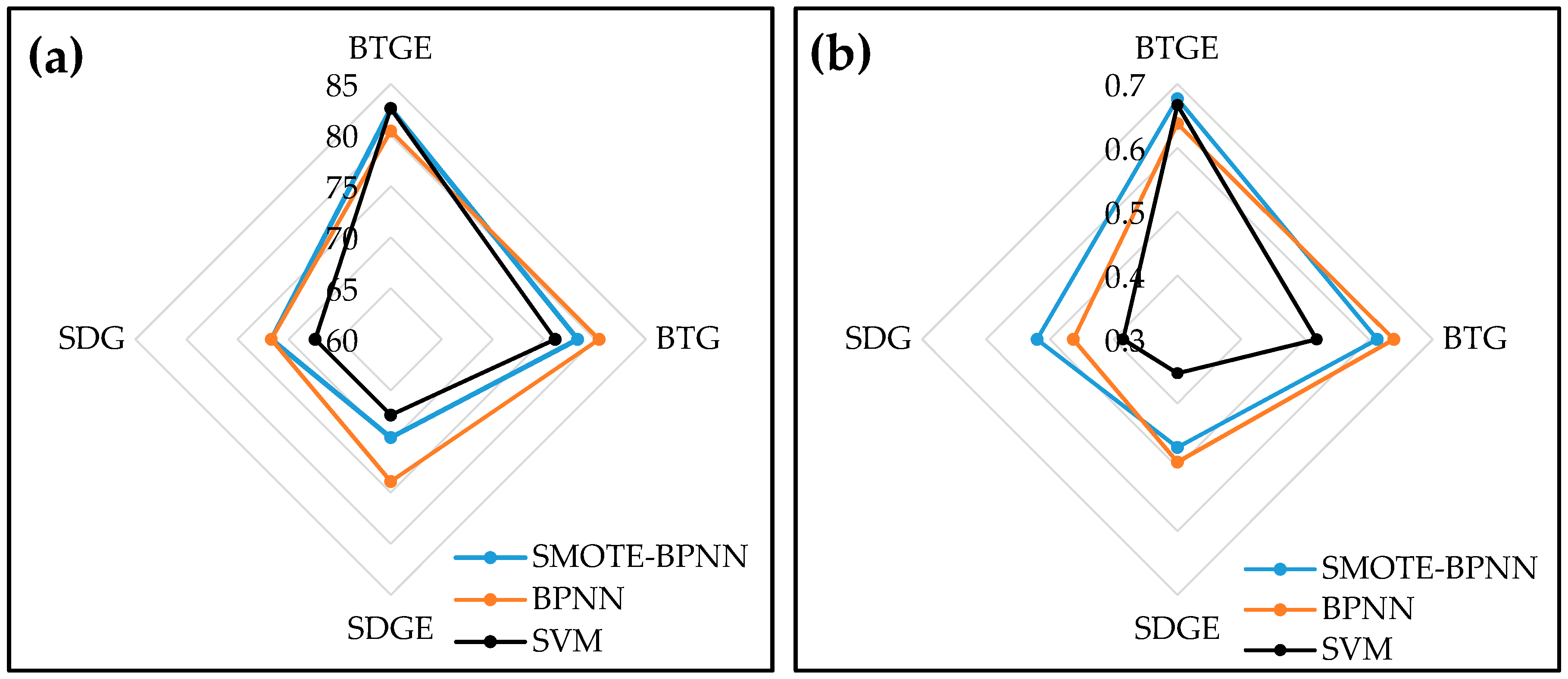
We found that classification using bi-temporal growth indices and environmental factors resulted in the highest accuracies among the four different feature sets for discriminating healthy, powdery mildew infected, and aphid damaged winter wheat through the three methods. Only the SMOTE-BPNN model obtained acceptable results for all three classes (i.e., healthy, powdery mildew infected, and aphid damaged) among the three SDG-based models. The BTGE-based SMOTE-BPNN method was also found to produce the most accurate classification for the two minority classes (i.e., healthy and aphid damaged). This suggests that our proposed SMOTE-BPNN method combing bi-temporal growth and environmental parameters improved overall crop disease and pest discriminating accuracy.

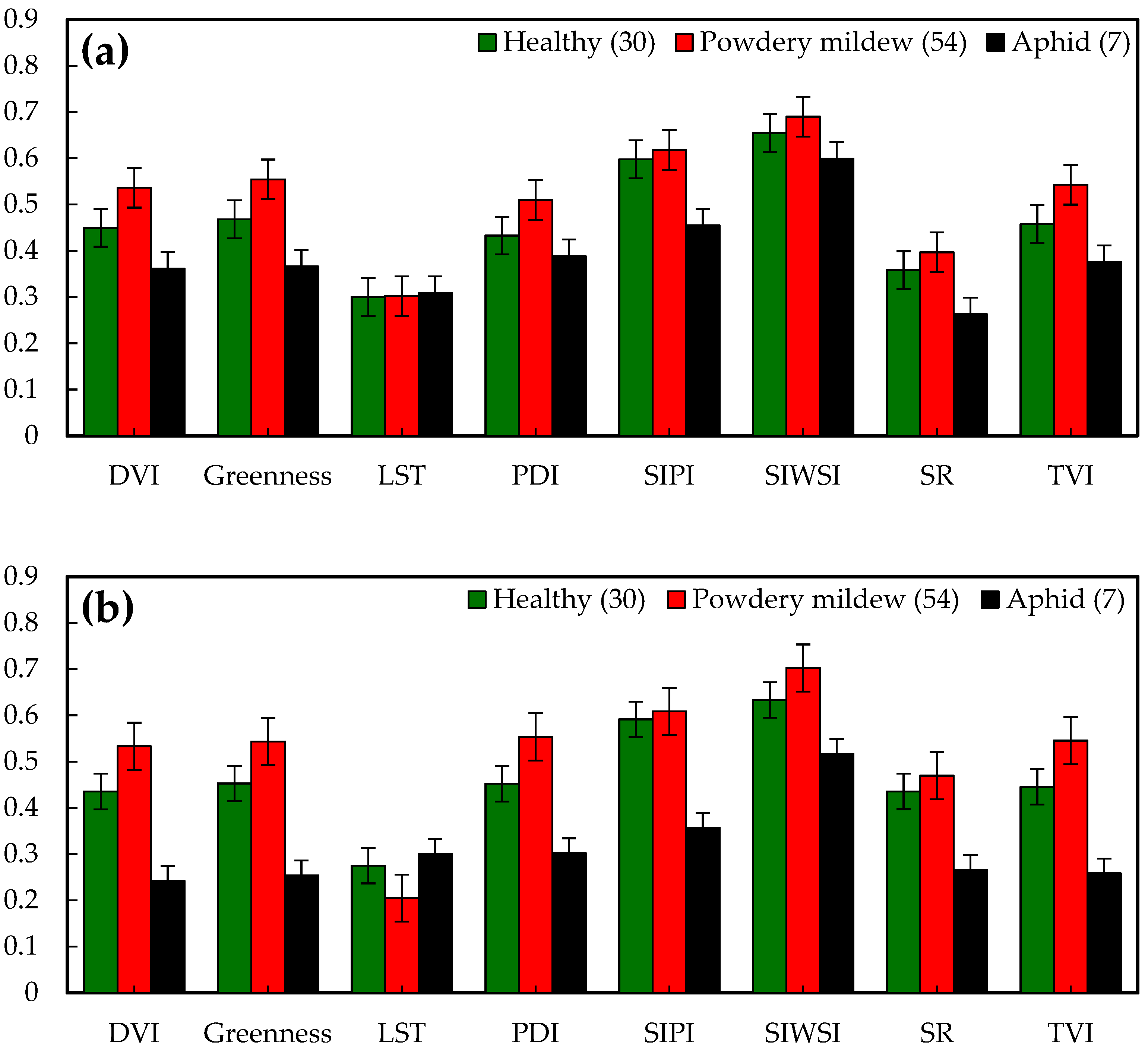
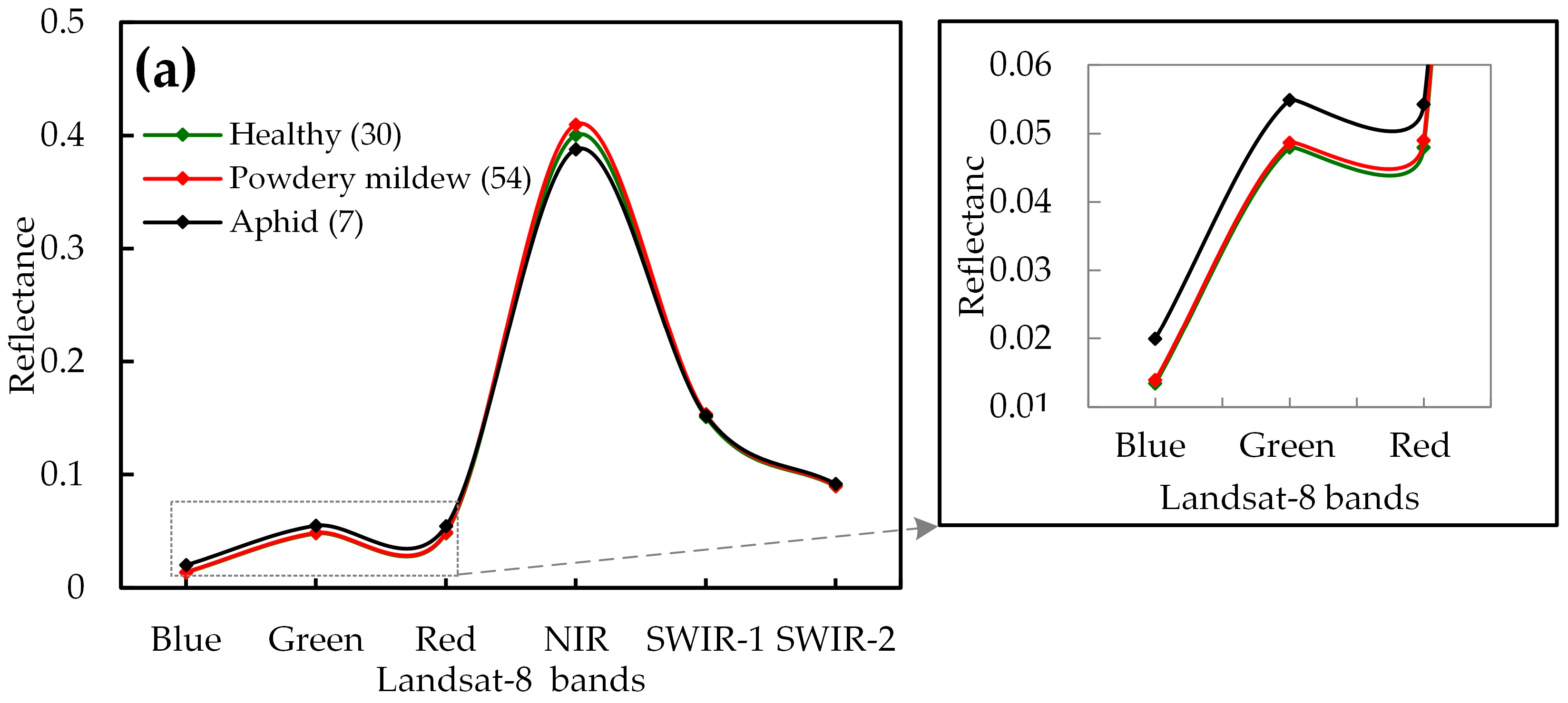
Typically, the disease causes the changes of biophysical and biochemical parameters of plants, such as pigments, water content and canopy structure as well as leaf color changes due to pustules or lesions [72]. Meanwhile, pest damages can also cause a reduction in pigment concentrations especially chlorophylls and leaf water content in the infested leaf and the destruction of infested leaf tissues [6,73]. These changes can influence the tissue optical properties and alter the spectral response characteristics [13,74,75]. The reduction of chlorophyll concentrations and water content in the leaf, damaged by aphids piercing the leaf and sucking out leaf juice, results in a higher reflectance in the visible and SWIR regions than the non-infested leaf [6]. The leaf tissue destructed by aphid infestation leads to a lower reflectance than the non-infested leaf in the NIR region [73]. The raw reflectance of leaves diseased by powdery mildew has a significant increase in the visible spectral region and a slight decrease in the NIR region over that of the healthy wheat leaves. Similar spectral characteristics of powdery mildew and aphids were also observed in the present study (Figure 7). The chosen indices (i.e., DVI, PDI, SIPI, SIWSI, SR and TVI) exhibit remarkable performance on monitoring and discriminating powdery mildew and aphids. These indices enable transformation of raw spectra into more meaningful metrics of the disease and pest damage. Furthermore, two environmental factors LST and Greenness had also been used for discriminating wheat disease and pest in this study. Their contributions for classification was evaluated. LST extracted from satellite imagery has been identified as one of the sky parameters controlling the physical, chemical, and biological processes at the interface between the earth and the atmosphere [76,77]. LST is also an effective means of partitioning latent heat fluxes, which provides information on micro-environmental conditions such as crop respiration and evapotranspiration [19,78]. Meanwhile, Greenness is responsive to the characteristic of healthy green vegetation that has high absorption of chlorophyll in the visible region and high reflectance of leaf tissue in the NIR region, so it reflects overall crop growth conditions and is suitable for the characterization of field environment [19,79]. These two environmental parameters influence the occurrence of crop diseases and pests. Our results revealed the relationship between the environmental factors and the development of the crop conditions affected by the disease and pest (Figure 3) and demonstrated the positive contributions of environmental factors for the discrimination of different diseases and pests (Figure 5, Table A2, Table A3 and Table A4).

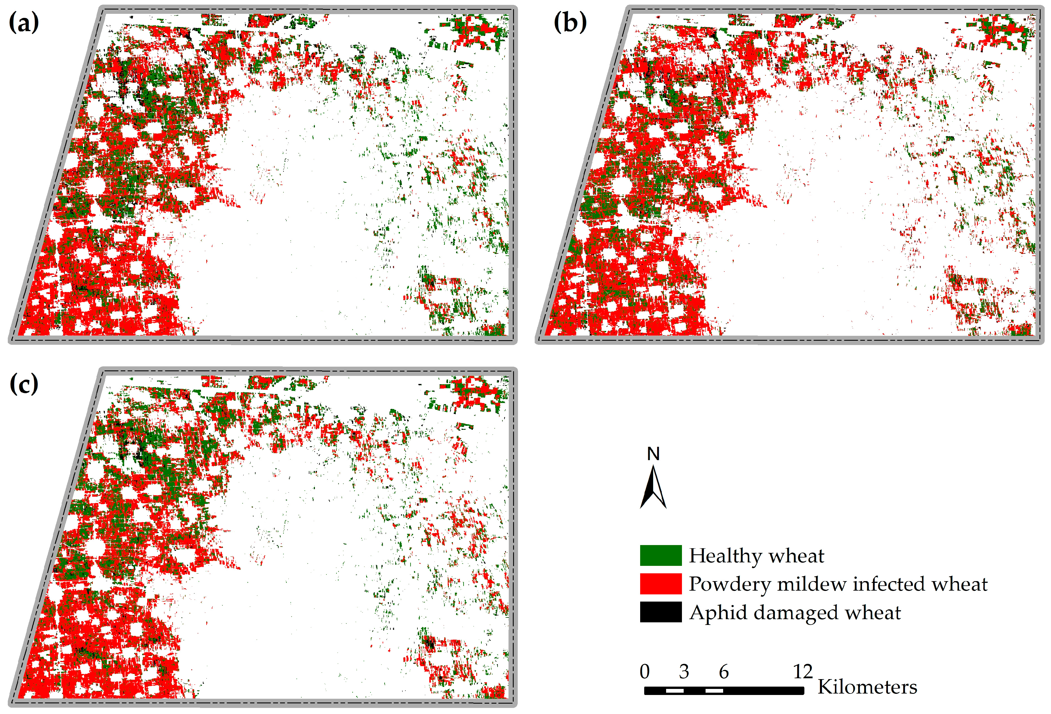
Compared with single-date feature sets, the newly proposed bi-temporal feature sets performed better on discriminating and mapping healthy wheat, powdery mildew infected and aphid infested wheat (Figure 5, Table A2, Table A3 and Table A4). Factors such as phenological, cultivation, and crop conditions may lead to responses of the same features which fluctuate following the disease and pest infestations [80]. The occurrence and development characteristics of different diseases and pests are different. The bi-temporal variations help to eliminate field anomalies other than the disease and pest infestations [8]. For example, the bi-temporal features could characterize the pigments and canopy morphology variations better, and indicated the relative importance of the combination of multi-temporal features in discriminating crop disease and pest. Currently, the quick development of precision agriculture requires finer field details and higher temporal resolutions. Due to the special location of the study area, two scenes with a time interval of less than 16 days were successfully acquired. Hence, the Landsat-8 imagery was successfully used for the discrimination of the wheat disease and pest in this case study. Furthermore, although the dates of the image acquisition and field survey were very hard to keep consistent due to the influence of the sensor revisit period and cloud cover, the chosen investigation dates in this study were a critical period when the occurrence and development potential of crop disease and pest remained consistent and stable [41,42,43,81]. Therefore, the obtained samples could effectively reflect the occurrence and development of disease and pest, and our good results demonstrated such effectiveness of the samples. On the other hand, although some high spatial-temporal resolution satellite images (i.e., Worldview-2, PlanetScope, SPOT-6 and so on) have been used to monitor and discriminate different crop diseases and pests, the corresponding environmental characteristics cannot be obtained from these sensors due to the limitations of their available bands [8,13,19]. Therefore, in the future, field investigation and satellite acquisition dates should be as consistent as possible, and multi-source remote sensing data should be fused for crop disease and pest discrimination.

The feasibility of each type of remotely sensed feature sets in describing different crop damages was assessed using different feature combinations balanced by SMOTE as input variables in BPNN (SMOTE-BPNN). For disease and pest discrimination, the positive contributions of environmental information and the importance of the two temporal images were confirmed in this research by developing models using the four different feature sets (BTGE, BTG, SDGE, and SDG) (Figure 5). Based on the bi-temporal growth indices and environmental factors, all three methods (i.e., SMOTE-BPNN, BPNN and SVM) had similar overall accuracy values and the classification accuracies for the healthy plots were all acceptable for the three methods based on this feature set. However, the classification accuracy for the aphid damaged plots using SMOTE-BPNN increased by 25.0% compared with the accuracy using the other two methods. Meanwhile, the G-means of the SMOTE-BPNN model based on the feature set was 8.0% and 9.0% higher than that for BPNN and SVM, respectively (Table 6). The results proved that the bi-temporal growth indices and environmental factors-based SMOTE-BPNN were an effective approach for automatic discrimination among healthy wheat, powdery mildew infected wheat and aphid damaged wheat. This approach performed well in the classification of the small or rare classes. Additionally, although the imbalance of the training data had been improved by the SMOTE algorithm, it was not optimal (Table 5). The disadvantage of SMOTE reported is that, since the separation between majority and minority class clusters is not often clear, noisy samples may be generated, resulting in a new sample set that may not be the best one [82]. Some modifications of SMOTE have been proposed [83,84]. Therefore, more suitable methods for imbalanced data should be further studied for application to the discrimination of imbalanced crop diseases and pests.

Overall, the proposed SMOTE-BPNN model integrating bi-temporal growth indices and environmental factors performed better in discriminating damages in winter wheat based on Landsat-8 satellite imagery, with a good accuracy of 82.6%. In this study, our goals were to improve the accuracy of the discrimination models through the integration of multi-source and multi-temporal remotely sensed data, thus providing a detailed spatial distribution of crop diseases and pests to meet the current needs of precision agriculture. Meanwhile, the combination of the SMOTE resample algorithm and the BPNN classification method made the classification of imbalanced data more accurate. However, limited by the spatial-temporal resolution of Landsat-8 images, although typical areas of diseases or pests infestation were firstly chosen and a diagonal five point sampling method based on the combination scheme of random sampling and representative sampling was then used to characterize the damage severity of each sample plot, it is still very difficult to eliminate the influence of the mixed pixel problem. In addition, our research was based solely on remote sensing data. In future research, multi-source information such as climate data and geographic data that are able to eliminate the classification uncertainty should also be incorporated. Some satellite data with finer spatial-temporal resolution should also be used in crop pest and disease monitoring and discrimination by fusing medium resolution satellite data containing environmental information. Additionally, more advanced methods that are more sensitive to imbalanced data can be tested to further improve the stability and reliability on crop disease and pest discrimination.

5. Conclusions

This study developed a BTGE-based SMOTE-BPNN approach using Landsat-8 imagery to discriminate powdery mildew and aphids in winter wheat. Compared with the traditional SDG-based method, the overall accuracy of the proposed approach (82.6%) had increased by 10.9%. A combination of bi-temporal growth and environmental parameters could accurately characterize the regional spatial distribution of crop diseases and pests and thus can provide technical support for field disease prevention and management. Furthermore, the combination of SMOTE and BPNN improved the classification accuracy for the three wheat classes (i.e., healthy, powdery mildew infected, and aphid damaged). Future studies should explore the fusion of multi-source remote sensing data such as Landsat-8 and Worldview-2 and the incorporation of physiological parameters to improve the performance and robustness of the crop disease and pest discrimination techniques.

References

1. Huang, X.Q.; Hsam, S.L.K.; Zeller, F.J.; Wenzel, G.; Mohler, V. Molecular mapping of the wheat powdery mildew resistance gene Pm24 and marker validation for molecular breeding. Theor. Appl. Genet. 2000, 101, 407–414. [Google Scholar] [CrossRef]
2. Luo, J.; Wang, D.; Dong, Y.; Huang, W.; Wang, J. Developing an aphid damage hyperspectral index for detecting aphid (Hemiptera: Aphididae) damage levels in winter wheat. In Proceedings of the Geoscience and Remote Sensing Symposium, Vancouver, BC, Canada, 24–29 July 2011; pp. 1744–1747. [Google Scholar]
3. Zhang, J.; Pu, R.; Yuan, L.; Huang, W.; Nie, C.; Yang, G. Integrating Remotely Sensed and Meteorological Observations to Forecast Wheat Powdery Mildew at a Regional Scale. IEEE J. Sel. Top. Appl. Earth Obs. Remote Sens. 2014, 7, 4328–4339. [Google Scholar] [CrossRef]
4. Shi, Y.; Huang, W.; Zhou, X. Evaluation of wavelet spectral features in pathological detection and discrimination of yellow rust and powdery mildew in winter wheat with hyperspectral reflectance data. J. Appl. Remote Sens. 2017, 11, 026025. [Google Scholar] [CrossRef]
5. Larsson, H. A crop loss model and economic thresholds for the grain aphid, Sitobion avenae (F.), in winter wheat in southern Sweden. Crop Prot. 2005, 24, 397–405. [Google Scholar] [CrossRef]
6. Luo, J.; Huang, W.; Yuan, L.; Zhao, C.; Du, S.; Zhang, J.; Zhao, J. Evaluation of spectral indices and continuous wavelet analysis to;quantify aphid infestation in wheat. Precis. Agric. 2013, 14, 151–161. [Google Scholar] [CrossRef]
7. Wang, K.; Liu, J.; Zhan, Y.; Liu, Y. A new slow-release formulation of methyl salicylate optimizes the alternative control of Sitobion avenae (Fabricius) (Hemiptera: Aphididae) in wheat fields. Pest Manag. Sci. 2018, 3, 676–682. [Google Scholar] [CrossRef] [PubMed]
8. Shi, Y.; Huang, W.; Ye, H.; Ruan, C.; Xing, N.; Geng, Y.; Dong, Y.; Peng, D. Partial Least Square Discriminant Analysis Based on Normalized Two-Stage Vegetation Indices for Mapping Damage from Rice Diseases Using PlanetScope Datasets. Sensors 2018, 18, 1901. [Google Scholar] [CrossRef] [PubMed]
9. Feng, W.; Shen, W.; He, L.; Duan, J.; Guo, B.; Li, Y.; Wang, C.; Guo, T. Improved remote sensing detection of wheat powdery mildew using dual-green vegetation indices. Precis. Agric. 2016, 17, 608–627. [Google Scholar] [CrossRef]
10. Riedell, W.E.; Blackmer, T.M. Leaf reflectance spectra of cereal aphid-damaged wheat. Crop Sci. 1999, 39, 1835–1840. [Google Scholar] [CrossRef]
11. Huang, W.; Guan, Q.; Luo, J.; Zhang, J.; Zhao, J.; Liang, D.; Huang, L.; Zhang, D. New Optimized Spectral Indices for Identifying and Monitoring Winter Wheat Diseases. IEEE J. Sel. Top. Appl. Earth Obs. Remote Sens. 2014, 7, 2516–2524. [Google Scholar] [CrossRef]
12. Yuan, L.; Zhang, H.; Zhang, Y.; Xing, C.; Bao, Z. Feasibility assessment of multi-spectral satellite sensors in monitoring and discriminating wheat diseases and insects. Opt. Int. J. Light Electron Opt. 2017, 131, 598–608. [Google Scholar] [CrossRef]
13. Yuan, L.; Zhang, J.; Shi, Y.; Nie, C.; Wei, L.; Wang, J. Damage mapping of powdery mildew in winter wheat with high-resolution satellite image. Remote Sens. 2014, 6, 3611–3623. [Google Scholar] [CrossRef]
14. Ma, H.; Jing, Y.; Huang, W.; Shi, Y.; Dong, Y.; Zhang, J.; Liu, L. Integrating Early Growth Information to Monitor Winter Wheat Powdery Mildew Using Multi-Temporal Landsat-8 Imagery. Sensors 2018, 18, 3290. [Google Scholar] [CrossRef]
15. Luo, J.; Zhao, C.; Huang, W.; Zhang, J.; Zhao, J.; Dong, Y.; Yuan, L.; Du, S. Discriminating wheat aphid damage degree using 2-dimensional feature space derived from landsat 5 TM. Sens. Lett. 2012, 10, 608–614. [Google Scholar] [CrossRef]
16. Mirik, M.; Ansley, R.J.; Price, J.A.; Workneh, F.; Rush, C.M. Remote monitoring of wheat streak mosaic progression using sub-pixel classification of Landsat 5 TM imagery for site specific disease management in winter wheat. Adv. Remote Sens. 2013, 2, 16. [Google Scholar] [CrossRef]
17. Navrozidis, I.; Alexandridis, T.K.; Dimitrakos, A.; Lagopodi, A.L.; Moshou, D.; Zalidis, G. Identification of purple spot disease on asparagus crops across spatial and spectral scales. Comput. Electron. Agric. 2018, 148, 322–329. [Google Scholar] [CrossRef]
18. Zhang, J.; Yuan, L.; Nie, C.; Wei, L.; Yang, G. Forecasting of powdery mildew disease with multi-sources of remote sensing information. In Proceedings of the Third International Conference on Agro-Geoinformatics (Agro-Geoinformatics 2014), Beijing, China, 11–14 August 2014; pp. 1–5. [Google Scholar]
19. Yuan, L.; Bao, Z.; Zhang, H.; Zhang, Y.; Liang, X. Habitat monitoring to evaluate crop disease and pest distributions based on multi-source satellite remote sensing imagery. Optik 2017, 145, 66–73. [Google Scholar] [CrossRef]
20. Ma, H.; Huang, W.; Jing, Y.; Dong, Y.; Zhang, J.; Nie, C.; Tang, C.; Zhao, J.; Huang, L. Remote sensing monitoring of wheat powdery mildew based on AdaBoost model combining mRMR algorithm. Trans. Chin. Soc. Agric. Eng. 2017, 33, 162–169. [Google Scholar]
21. Oumar, Z.; Mutanga, O. Using WorldView-2 bands and indices to predict bronze bug (Thaumastocoris peregrinus) damage in plantation forests. Int. J. Remote Sens. 2013, 34, 2236–2249. [Google Scholar] [CrossRef]
22. Yuan, L.; Pu, R.; Zhang, J.; Wang, J.; Yang, H. Using high spatial resolution satellite imagery for mapping powdery mildew at a regional scale. Precis. Agric. 2016, 17, 332–348. [Google Scholar] [CrossRef]
23. Zhang, C.; Guo, J.; Lu, J. Research on Classification Method of High-Dimensional Class-Imbalanced Data Sets Based on SVM. In Proceedings of the IEEE Second International Conference on Data Science in Cyberspace, Shenzhen, China, 26–29 June 2017; pp. 60–67. [Google Scholar]
24. Provost, F. Machine learning from imbalanced data sets 101. In Proceedings of the AAAI’2000 Workshop on Imbalanced Data Sets, Austin, TX, USA, 31 July 2000; pp. 1–3. [Google Scholar]
25. Huang, Y.-M.; Hung, C.-M.; Jiau, H.C. Evaluation of neural networks and data mining methods on a credit assessment task for class imbalance problem. Nonlinear Anal. Real World Appl. 2006, 7, 720–747. [Google Scholar] [CrossRef]
26. Chawla, N.V.; Bowyer, K.W.; Hall, L.O.; Kegelmeyer, W.P. SMOTE: Synthetic minority over-sampling technique. J. Artif. Intell. Res. 2002, 16, 321–357. [Google Scholar] [CrossRef]
27. Wang, Q.; Luo, Z.; Huang, J.; Feng, Y.; Liu, Z. A novel ensemble method for imbalanced data learning: Bagging of extrapolation-SMOTE SVM. Comput. Intell. Neurosci. 2017, 2017, 1827016. [Google Scholar] [CrossRef]
28. Liu, X.-Y.; Wu, J.; Zhou, Z.-H. Exploratory undersampling for class-imbalance learning. IEEE Trans. Syst. Man Cybern. Part B (Cybern.) 2009, 39, 539–550. [Google Scholar]
29. Zhang, G.; Patuwo, B.E.; Hu, M.Y. Forecasting with artificial neural networks: The state of the art. Int. J. Forecast. 1998, 14, 35–62. [Google Scholar] [CrossRef]
30. Wang, L.; Zeng, Y.; Chen, T. Back propagation neural network with adaptive differential evolution algorithm for time series forecasting. Expert Syst. Appl. 2015, 42, 855–863. [Google Scholar] [CrossRef]
31. Aslanargun, A.; Mammadov, M.; Yazici, B.; Yolacan, S. Comparison of ARIMA, neural networks and hybrid models in time series: Tourist arrival forecasting. J. Stat. Comput. Simul. 2007, 77, 29–53. [Google Scholar] [CrossRef]
32. Jiang, P.; Ge, Y.; Wang, C. Research and application of a hybrid forecasting model based on simulated annealing algorithm: A case study of wind speed forecasting. J. Renew. Sustain. Energy 2016, 8, 015501. [Google Scholar] [CrossRef]
33. Liu, M.; Wang, M.; Wang, J.; Li, D. Comparison of random forest, support vector machine and back propagation neural network for electronic tongue data classification: Application to the recognition of orange beverage and Chinese vinegar. Sens. Actuators B Chem. 2013, 177, 970–980. [Google Scholar] [CrossRef]
34. Shifali; Kaur, G. Satellite Image Classification using Back Propagation Neural Network. Indian J. Sci. Technol. 2016, 9. [Google Scholar] [CrossRef]
35. Zin, A.A.M.; Saini, M.; Mustafa, M.W.; Sultan, A.R. New algorithm for detection and fault classification on parallel transmission line using DWT and BPNN based on Clarke’s transformation. Neurocomputing 2015, 168, 983–993. [Google Scholar]
36. Mouazen, A.; Kuang, B.; De Baerdemaeker, J.; Ramon, H. Comparison among principal component, partial least squares and back propagation neural network analyses for accuracy of measurement of selected soil properties with visible and near infrared spectroscopy. Geoderma 2010, 158, 23–31. [Google Scholar] [CrossRef]
37. Feng, Y.; Zhang, W.; Sun, D.; Zhang, L. Ozone concentration forecast method based on genetic algorithm optimized back propagation neural networks and support vector machine data classification. Atmos. Environ. 2011, 45, 1979–1985. [Google Scholar] [CrossRef]
38. Zhou, J.; Zhang, Y.; Zhou, A.; Liu, C.; Cai, H.; Liu, Y. Application of hydrochemistry and stable isotopes (δ34S, δ18O and δ37Cl) to trace natural and anthropogenic influences on the quality of groundwater in the piedmont region, Shijiazhuang, China. Appl. Geochem. 2016, 71, 63–72. [Google Scholar] [CrossRef]
39. Niu, J.; Zhang, W.; Ru, S.; Chen, X.; Xiao, K.; Zhang, X.; Assaraf, M.; Imas, P.; Magen, H.; Zhang, F. Effects of potassium fertilization on winter wheat under different production practices in the North China Plain. Field Crops Res. 2013, 140, 69–76. [Google Scholar] [CrossRef]
40. Liu, L.; Dong, Y.; Huang, W.; Du, X.; Luo, J.; Shi, Y.; Ma, H. Enhanced Regional Monitoring of Wheat Powdery Mildew Based on an Instance-Based Transfer Learning Method. Remote Sens. 2019, 11, 298. [Google Scholar] [CrossRef]
41. Wang, X.D.; Ma, Y.Z.; Chen, X.B.; Zhang, A.M.; Fu, L.J. Occurrence and Critical Controlling Period of Wheat Aphids in Tangshan. Heilongjiang Agric. Sci. 2016, 6, 68–71. [Google Scholar]
42. Wiese, M.V. Compendium of wheat diseases. Soil Sci. 1978, 126, 190. [Google Scholar] [CrossRef]
43. Te Beest, D.E.; Paveley, N.D.; Shaw, M.W.; Van Den Bosch, F. Disease-weather relationships for powdery mildew and yellow rust on winter wheat. Phytopathology 2008, 98, 609–617. [Google Scholar] [CrossRef]
44. Zhang, J.; Pu, R.; Yuan, L.; Wang, J.; Huang, W.; Yang, G. Monitoring powdery mildew of winter wheat by using moderate resolution multi-temporal satellite imagery. PLoS ONE 2014, 9, e93107. [Google Scholar] [CrossRef]
45. Li, Z.G.; Yang, P.; Zhou, Q.B.; Wang, Y.; Wu, W.B.; Zhang, L.; Zhang, X. Research on spatiotemporal pattern of crop phenological characteristics and cropping system in North China based on NDVI time series data. Acta Ecol. Sin. 2009, 29, 6216–6226. [Google Scholar]
46. Li, C.; Wang, J.; Liu, L.; Song, X.; Wang, R. Land cover mapping of winter wheat and clover using muti-temporal Landsat NIR band in a growing season. Trans. Chin. Soc. Agric. Eng. 2005, 21, 256–268. [Google Scholar]
47. Baig, M.H.A.; Zhang, L.; Tong, S.; Tong, Q. Derivation of a tasselled cap transformation based on Landsat 8 at-satellite reflectance. Remote Sens. Lett. 2014, 5, 423–431. [Google Scholar] [CrossRef]
48. Jordan, C.F. Derivation of Leaf-Area Index from Quality of Light on the Forest Floor. Ecology 1969, 50, 663–666. [Google Scholar] [CrossRef]
49. Qin, Q.; Ghulam, A.; Zhu, L.; Wang, L.; Li, J.; Nan, P. Evaluation of MODIS derived perpendicular drought index for estimation of surface dryness over northwestern China. Int. J. Remote Sens. 2008, 29, 1983–1995. [Google Scholar] [CrossRef]
50. Peñuelas, J.; Inoue, Y. Reflectance Indices Indicative of Changes in Water and Pigment Contents of Peanut and Wheat Leaves. Photosynthetica 1999, 36, 355–360. [Google Scholar] [CrossRef]
51. Olsen, J.L.; Ceccato, P.; Proud, S.R.; Fensholt, R.; Grippa, M.; Mougin, E.; Ard, J.; Sandholt, I. Relation between Seasonally Detrended Shortwave Infrared? Reflectance Data and Land Surface Moisture in Semi-Arid Sahel. Remote Sens. 2013, 5, 2898–2927. [Google Scholar] [CrossRef]
52. Peñuelas, J.; Filella, I. Visible and near-infrared reflectance techniques for diagnosing plant physiological status. Trends Plant Sci. 1998, 3, 151–156. [Google Scholar] [CrossRef]
53. Calero, A.D.T.; Nieto, H.; Guzinski, R.; Mendiguren, G.; Sandholt, I.; Berliner, P. Multi-scale approach of the surface temperature/vegetation index triangle method for estimating evapotranspiration over heterogeneous landscapes. In Proceedings of the EGU General Assembly, Vienna, Austria, 22–27 April 2012; p. 697. [Google Scholar]
54. Chander, G.; Markham, B.L.; Helder, D.L. Summary of current radiometric calibration coefficients for Landsat MSS, TM, ETM+, and EO-1 ALI sensors. Remote Sens. Environ. 2009, 113, 893–903. [Google Scholar] [CrossRef]
55. Hao, P.; Niu, Z.; Zhan, Y.; Wu, Y.; Wang, L.; Liu, Y. Spatiotemporal changes of urban impervious surface area and land surface temperature in Beijing from 1990 to 2014. GISci. Remote Sens. 2016, 53, 63–84. [Google Scholar] [CrossRef]
56. Sui, Y.; Wei, Y.; Zhao, D. Computer-aided lung nodule recognition by SVM classifier based on combination of random undersampling and SMOTE. Comput. Math. Methods Med. 2015, 2015, 368674. [Google Scholar] [CrossRef]
57. Pears, R.; Finlay, J.; Connor, A.M. Synthetic Minority over-sampling technique (SMOTE) for predicting software build outcomes. arXiv, 2014; arXiv:1407.2330. [Google Scholar]
58. Bifet, A.; Holmes, G.; Kirkby, R.; Pfahringer, B. MOA: Massive Online Analysis. J. Mach. Learn. Res. 2010, 11, 1601–1604. [Google Scholar]
59. Drown, D.J.; Khoshgoftaar, T.M.; Seliya, N. Evolutionary Sampling and Software Quality Modeling of High-Assurance Systems. IEEE Trans. Syst. Man Cybern. Part A Syst. Hum. 2009, 39, 1097–1107. [Google Scholar] [CrossRef]
60. Ding, S.; Yu, J. An optimizing BP neural network algorithm based on genetic algorithm. Artif. Intell. Rev. 2011, 36, 153–162. [Google Scholar] [CrossRef]
61. Chen, K.; Yang, S.; Batur, C. Effect of multi-hidden-layer structure on performance of BP neural network: Probe. In Proceedings of the 2012 8th International Conference on Natural Computation, Chongqing, China, 29–31 May 2012; pp. 1–5. [Google Scholar]
62. Yang, S.J.; Chen, K. Effect of Multi-hidden-layer on Performance of BP Neural Network. J. Ningbo Univ. 2013, 26, 48–52. [Google Scholar]
63. Blum, A. Neural Networks in C++: An Object-Oriented Framework for Building Connectionist Systems; John Wiley & Sons, Inc.: Hoboken, NK, USA, 1992. [Google Scholar]
64. Shi, Y.; Zhao, X.-T.; Zhang, Y.-M.; Ren, N.-Q. Back propagation neural network (BPNN) prediction model and control strategies of methanogen phase reactor treating traditional Chinese medicine wastewater (TCMW). J. Biotechnol. 2009, 144, 70–74. [Google Scholar] [CrossRef]
65. Liu, C.; Frazier, P.; Kumar, L. Comparative assessment of the measures of thematic classification accuracy. Remote Sens. Environ. 2007, 107, 606–616. [Google Scholar] [CrossRef]
66. Bekkar, M.; Djemaa, H.K.; Alitouche, T.A. Evaluation measures for models assessment over imbalanced datasets. J. Inf. Eng. Appl. 2013, 3. [Google Scholar]
67. Wu, M.; Hou, L.; Yang, D.; School, C. Improved AdaBoost algorithm based on multi-class unbalance classification. J. Beijing Inf. Sci. Technol. Univ. 2018, 33, 76–81. [Google Scholar]
68. Fawcett, T. An introduction to ROC analysis. Pattern Recognit. Lett. 2006, 27, 861–874. [Google Scholar] [CrossRef]
69. Hido, S.; Kashima, H.; Takahashi, Y. Roughly balanced bagging for imbalanced data. Stat. Anal. Data Min. ASA Data Sci. J. 2009, 2, 412–426. [Google Scholar] [CrossRef]
70. Story, M.; Congalton, R.G. Accuracy assessment: A user’s perspective. Photogramm. Eng. Remote Sens. 1986, 52, 397–399. [Google Scholar]
71. Rosenfield, G.H.; Fitzpatrick-Lins, K. A coefficient of agreement as a measure of thematic classification accuracy. Photogramm. Eng. Remote Sens. 1986, 52, 223–227. [Google Scholar]
72. Sankaran, S.; Mishra, A.; Ehsani, R.; Davis, C. A review of advanced techniques for detecting plant diseases. Comput. Electron. Agric. 2010, 72, 1–13. [Google Scholar] [CrossRef]
73. Graeff, S.; Claupein, W. Identification and discrimination of water stress in wheat leaves (Triticum aestivum L.) by means of reflectance measurements. Irrig. Sci. 2007, 26, 61–70. [Google Scholar] [CrossRef]
74. Broge, N.H.; Mortensen, J.V. Deriving green crop area index and canopy chlorophyll density of winter wheat from spectral reflectance data. Remote Sens. Environ. 2002, 81, 45–57. [Google Scholar] [CrossRef]
75. Ayala-Silva, T.; Beyl, C.A. Changes in spectral reflectance of wheat leaves in response to specific macronutrient deficiency. Adv. Space Res. Off. J. Comm. Space Res. 2005, 35, 305–317. [Google Scholar] [CrossRef]
76. Voogt, J.A.; Oke, T.R. Thermal remote sensing of urban climates. Remote Sens. Environ. 2003, 86, 370–384. [Google Scholar] [CrossRef]
77. Small, C. Comparative analysis of urban reflectance and surface temperature. Remote Sens. Environ. 2006, 104, 168–189. [Google Scholar] [CrossRef]
78. Zhang, Y.; Odeh, I.O.A.; Han, C. Bi-temporal characterization of land surface temperature in relation to impervious surface area, NDVI and NDBI, using a sub-pixel image analysis. Int. J. Appl. Earth Obs. Geoinf. 2009, 11, 256–264. [Google Scholar] [CrossRef]
79. Liu, Q.; Guo, Y.; Liu, G.; Zhao, J. Classification of Landsat 8 OLI image using support vector machine with Tasseled Cap Transformation. In Proceedings of the International Conference on Natural Computation, Xiamen, China, 19–21 August 2014. [Google Scholar]
80. Liu, Z.Y.; Huang, J.F.; Shi, J.J.; Tao, R.X.; Zhou, W.; Zhang, L.L. Characterizing and estimating rice brown spot disease severity using stepwise regression, principal component regression and partial least-square regression. J. Zhejiang Univ. Sci. B 2007, 8, 738–744. [Google Scholar] [CrossRef]
81. Kang, H. Dynamic and control of wheat powdery mildew in Xingtang County, Hebei Province. Master’s Thesis, Chinese Academy of Agricultural Sciences Dissertation, Beijing, China, 2012. [Google Scholar]
82. He, H.; Garcia, E.A. Learning from imbalanced data. IEEE Trans. Knowl. Data Eng. 2008, 21, 1263–1284. [Google Scholar]
83. Douzas, G.; Bacao, F. Geometric SMOTE: Effective oversampling for imbalanced learning through a geometric extension of SMOTE. arXiv, 2017; arXiv:1709.07377. [Google Scholar]
84. Han, H.; Wang, W.-Y.; Mao, B.-H. Borderline-SMOTE: A new over-sampling method in imbalanced data sets learning. In Proceedings of the International Conference on Intelligent Computing, Hefei, China, 23–26 August 2005; pp. 878–887. [Google Scholar]
Figure 1. Location of the experimental fields.
Remotesensing 11 00846 g001
Figure 2. The basic principle of the synthetic minority oversample technique (SMOTE) algorithm.
Remotesensing 11 00846 g002
Figure 3. Flowchart for constructing discrimination model for powdery mildew and aphid using bi-temporal Landsat-8 imagery integrating growth indices and environmental factors at regional scales.
Remotesensing 11 00846 g003
Figure 4. Means and standard deviations of the selected normalized growth indices and environmental factors for both healthy and damaged (powdery mildew and aphids) plots on (a) 15 May and (b) 22 May.
Remotesensing 11 00846 g004
Figure 5. Radar charts of (a) overall accuracy (OA%) and (b) kappa coefficients of four different feature sets-based coupled models of synthetic minority oversample technique algorithm and back propagation neural network method (SMOTE-BPNN), BPNN models and support vector machine (SVM) models.
Remotesensing 11 00846 g005
Figure 6. Damage maps of winter wheat produced by (a) SMOTE-BPNN; (b) BPNN; and (c) SVM using a bi-temporal feature set integrating growth indices and environmental factors.
Remotesensing 11 00846 g006
Figure 7. The average spectral reflectance for both healthy and damaged (powdery mildew and aphids) plots across the Landsat-8 spectral bands on (a) 15 May and (b) 22 May.
Remotesensing 11 00846 g007aRemotesensing 11 00846 g007b