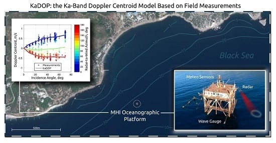
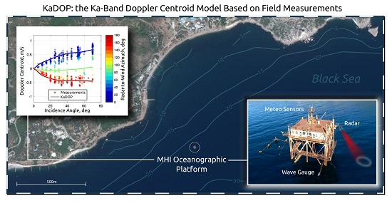
Sea Surface Ka-Band Doppler Measurements: Analysis and Model Development

Abstract

Multi-year field measurements of sea surface Ka-band dual-co-polarized (vertical transmit–receive polarization (VV) and horizontal transmit–receive polarization (HH)) radar Doppler characteristics from an oceanographic platform in the Black Sea are presented. The Doppler centroid (DC) estimated using the first moment of 5 min averaged spectrum, corrected for measured sea surface current, ranges between 0 and ≈1 m/s for incidence angles increasing from 0 to ${70}^{\circ }$. Besides the known wind-to-radar azimuth dependence, the DC can also depend on wind-to-dominant wave direction. For co-aligned wind and waves, a negative crosswind DC residual is found, ≈−0.1 m/s, at ≈20${}^{\circ }$ incidence angle, becoming negligible at ≈ 60${}^{\circ }$, and raising to, ≈+0.5 m/s, at ${70}^{\circ }$. For our observations, with a rather constant dominant wave length, the DC is almost wind independent. Yet, results confirm that, besides surface currents, the DC encodes an expected wave-induced contribution. To help the interpretation, a two-scale model (KaDOP) is proposed to fit the observed DC, based on the radar modulation transfer function (MTF) previously developed for the same data set. Assuming universal spectral shape of energy containing sea surface waves, the wave-induced DC contribution is then expressed as a function of MTF, significant wave height, and wave peak frequency. The resulting KaDOP agrees well with independent DC data, except for swell-dominated cases. The swell impact is estimated using the KaDOP with a modified empirical MTF.

1. Introduction

Today’s ocean radar scatterometry techniques are mainly based on the analysis of the sea surface backscattering intensity, or normalized radar cross-section (NRCS). Controlled by the surface roughness and look geometry, particularly local incidence angle at the surface, the NRCS can serve to retrieve the near-surface wind and/or wave characteristics, e.g., wind scatterometry [1], wave scatterometry [2], and/or be processed to provide very high-resolution wind and wave ocean surface information [3,4]. A novel approach to further extend scatterometer capabilities is to acquire and process the backscattering phase, or Doppler centroid (DC). The DC reflects the time evolution of backscattered fields, and thus encompasses the sea surface kinematics, including more direct information on underlying surface current properties.

Along-track interferometry (ATI) synthetic aperture radar (SAR) was first used to demonstrate the possibility to retrieve the sea surface currents from airborne radar data [5,6,7,8,9]. From space, the deviation between observed DC and expected DC due to satellite motion (so-called geophysical Doppler anomaly) was shown to quantitatively trace the sea surface currents [10,11,12,13]. The DC anomaly was also shown to help in resolving the wind direction ambiguity from SAR images [14,15].

As understood, a single high-resolution SAR image can only be inverted into the line-of-sight (radial) velocity component. A double-beam squinted interferometric SAR, the SEASTAR instrumental concept would resolve the full current vector [16,17]. A conventional scatterometer would be more energy-efficient than a SAR to provide continuous global observations, but the spatial resolution would be largely reduced. New concepts with multi-look (rotating beam) configuration for full vector retrieval are now under consideration by the European Space Agency (SKIM) [18,19] and the National Aeronautics and Space Administration (DopplerScatt/WaCM) [20,21]. In comparison with the existing altimetry-based current estimation, these instruments will have improved spatio-temporal resolution and capabilities to estimate the total ocean surface currents. This is the key for direct measurements of momentum fluxes relative to the moving ocean surface, better separation of geostrophic and ageostrophic current components, as well as further understanding of multiscale variability of the ocean circulation and its impacts on the vertical mixing and exchanges.

Similarly to wind retrieval from scatterometer data, the DC inversion can be performed via an empirical geophysical model functions (GMF), guided by theoretical models relating observed DC with environmental parameters and look geometry. Doppler scatterometry is relatively new, and there is no well-established quantitative description of the sea surface DC. Qualitatively, there exist a number of numerical simulations and quasi-analytical formulation of Doppler spectra and their moments [7,19,22,23,24,25,26,27,28,29,30].

Early field experiments in the North Sea, SAXON-FPN included radar measurements from L-band to Ka-band [31]. Doppler spectra from these experiments [32] can be used to estimate the Ka-band DC for incidence angles, $\theta =$ 50–80${}^{\circ }$. DC measurements were also performed in similar conditions from the Black Sea research platform for X-band at $\theta =$ 25–60${}^{\circ }$ and various sea states [33], and Ka-band at $\theta =$ 0–20${}^{\circ }$, but only at very light winds of 3–4 m/s [34].

The first global ocean Doppler GMF, the CDOP, has been constructed based on C-band ENVISAT ASAR data for $\theta =$ 17–42${}^{\circ }$ [14]. With the growing interest, several airborne experiments were carried out during the last several years. The proof-of-concept experiment for the SEASTAR concept used X-band SAR measurements at $\theta =$ 27–43${}^{\circ }$ [35]. The NASA DopplerScatt/WaCM airborne prototype yielded a Ka-band DC GMF at $\theta =$ 56${}^{\circ }$ [21]. Airborne flight data from AirSWOT, a precursor to the SWOT mission, provided Ka-band DC measurements at $\theta =$ 3–20${}^{\circ }$ to help demonstrate the SKIM design [19].

Note, all concepts [18,21,36,37] are considering Ka-band measurements as a reliable trade-off between atmospheric signal attenuation and higher spatial resolution, measurement accuracy, and smaller instrument size [38]. More precisely documenting Ka-band sea surface backscatter properties is thus timely.

Key to ocean Doppler data analysis is the fact that a Doppler radar measures the motion of the detected surface roughness element, rather than the current itself. The DC thus includes a detected scatter-induced DC component or, to simplify, a wave-induced component, which can be of the order of the current magnitude itself [19,35]. In this paper, to help document this wave-induced contribution, we continue presenting the results of multi-year field measurements performed from the Black Sea research platform. Following previous reports focusing on the mean NRCS [39] and its modulations by long surface waves [40,41], this paper addresses the Ka-band radar Doppler shift analysis.

The primary goal of this study is to present and analyze the Ka-band DC measurements, to develop their parameterization in a wide range of observational and environmental conditions, and thus make them usable to the community. The remainder of the paper is organized as follows. Section 2 describes the materials and methods used in the field experiments. In Section 3, we present the raw DC measurements as a function of look geometry and environmental variables. Using these data, in Section 4, we develop and validate a semi-empirical DC model which is based on a theoretical DC model (DopRIM [10,11,29]) and an empirical modulation transfer function [40]. In Section 5, we compare the semi-empirical model to other published results and discuss its features and applicability. Section 6 summarizes the results.

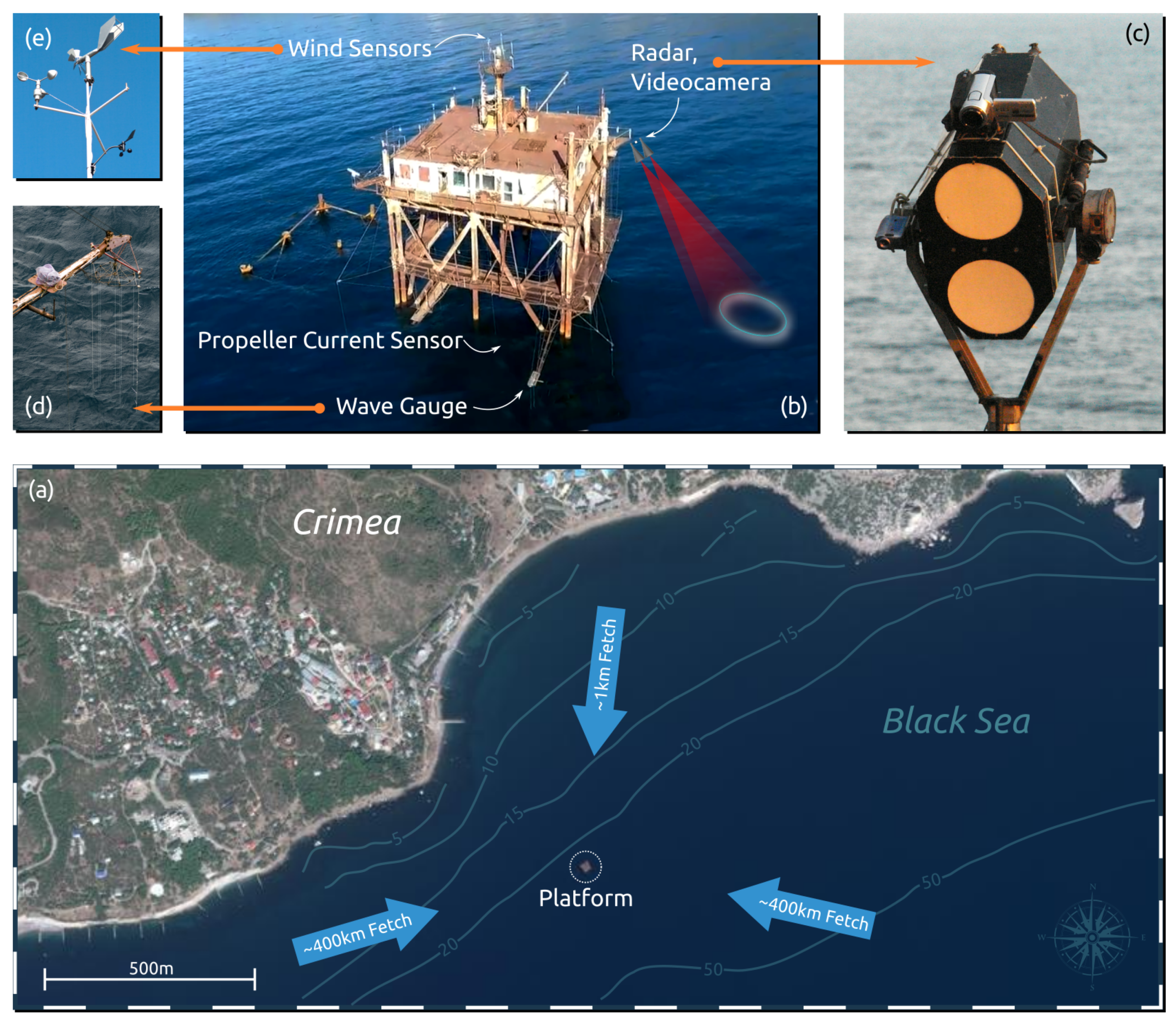
2. Materials and Methods

Experiments were conducted from the Black Sea oceanographic platform (Figure 1) operated by the Marine Hydrophysical Institute of the Russian Academy of Science. This is a truss-tower bottom fixed platform that locates 600 m offshore in a 30-m deep water (44${}^{\circ }$23′35″ N, 33${}^{\circ }$59′04″ E). The consideration is limited to onshore wind directions (easterly to south-westerly, 100 km < fetch $<400$ km) with typical peak wavelengths of ∼30–40 m at 10–15 m/s winds. Such wave conditions ensured applicability of the deep water wave approximation. The consideration was also limited to cases without a strong swell. Local currents typically varied from 0 to $0.3$–$0.5$ m/s.

2.1. Radar

Experiments were conducted with a Ka-band continuous-wave dual-co-polarized Doppler scatterometer (Figure 1c). It consisted of two co-aligned transmit/receive horn antennae separated by 22 cm. The radar operated at a hybrid polarization mode transmitting a wave of mixed polarization and receiving two orthogonal (vertical and horizontal) backscattering modes. This configuration implied a contamination of the co-polarized signals (vertical transmit–receive polarization (VV) and horizontal transmit–receive polarization (HH)) by cross-polarized signals, which were, however, very weak for typical wind conditions and can be disregarded (see Appendix B in [39] for more details).

Radar installation enabled us to vary the incidence angle, $\theta$, from 0 to 70${}^{\circ }$ with various radar-to-wind azimuths, but the pure downwind azimuth was rarely used to avoid platform wind shadowing impacts. At low/high incidence angles ($\theta$ less/more than ${45}^{\circ }$), the radar was installed on the top/bottom deck at 12/6-m height, respectively.

The two-way beam-width at a half-power level was 5/7${}^{\circ }$ in the vertical/horizontal plane for VV/HH polarization, respectively. The radar had a real aperture horn antenna. Its ground footprint size and position depended on the incidence angle and radar height only. For example, at low incidence angle observations from the top deck, the footprint size was ≈2 m by 2 m. At large $\theta =$ 70${}^{\circ }$ observations from the bottom beck the footprint size increased up to ≈3 m by 8 m (see Appendix A in [40] for more details).

The radar employs the homodyne method to extract the Doppler shift. Along with received power calibration, a special test was conducted to evaluate the transmitter oscillator instability and check its impact on the sea surface Doppler shift measurements [41]. Detected Doppler signals (I/Q pair per polarization) were digitized by an analog-to-digital converter at 40 kHz/channel sampling frequency. The Fourier transform of the recorded I/Q data was performed over 0.2 s time intervals yielding quasi-instantaneous Doppler spectra of the raw signal. Then, these spectra were averaged over a five minute interval to estimate mean Doppler spectrum for each five minute interval.

2.2. Hydro-Meteorological Measurements

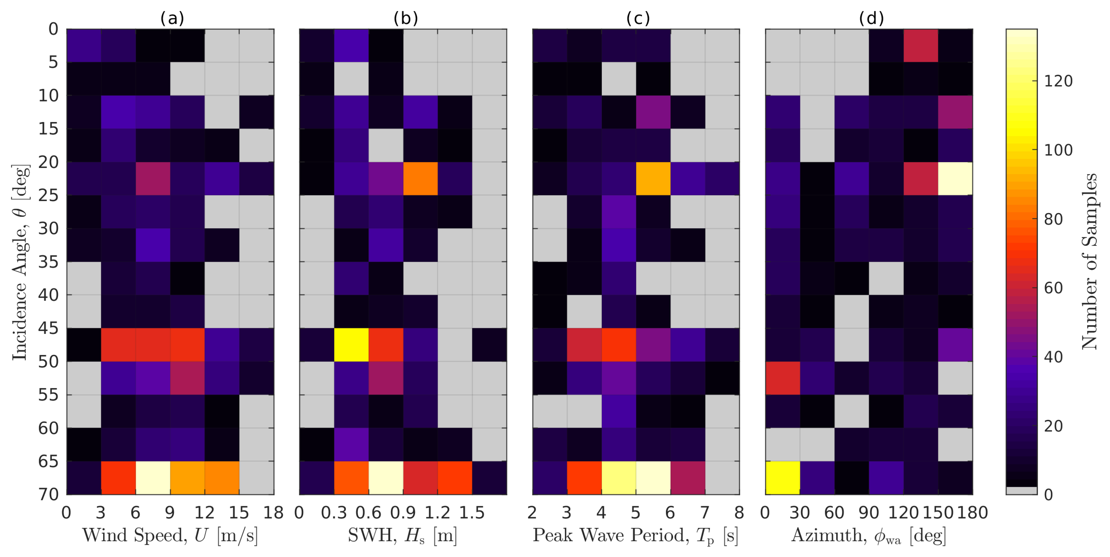
Supplementary instruments included the standard meteorological sensors installed at 23 m height mast (Figure 1e): wind anemometer, atmosphere temperature, humidity, and pressure. The water temperature sensor was submerged at 3 m depth. The data from meteorological sensors were used to estimate wind speed, U, at the standard 10 m height using the COARE 3.0 algorithm [42]. Currents at 10-m depth were measured by a propeller sensor. Surface waves were measured by the six-wire wave gauge antenna (Figure 1b). The wires were fixed at the center and vertices of a pentagon with 25-cm length edges. Directional frequency elevation spectra were estimated using the extended maximum likelihood method implemented in the DIWASP package [43].

Because Doppler scatterometers were designed to retrieve the surface currents, the standard 10 m depth propeller measurements were augmented by surface currents estimated from video records [44]. The video data were recorded by a digital video camera installed atop the radar and directed into its footprint (incidence angle 0–70${}^{\circ }$). The camera viewing angles were 28${}^{\circ }$/${47}^{\circ }$ in the vertical/horizontal planes, the frame rate is 25 Hz, and the image size was 1440 by 1080 pixels. In order to retrieve the sea surface currents, the Particle Image Velocimetry (PIV) technique (bubble tracking), along with the dispersion relation analysis were used. It was found that the PIV-derived currents are $ϵ=0.75\%U$ faster than the dispersion-derived currents, which, it turn, were $ϵ=1.3\%U$ faster than the 10m-depth propeller currents, where U is the 10 m neutral wind speed.

For radar data analysis, the currents derived from the wave dispersion analysis were used by default. If this estimate was unavailable (e.g., unsuccessful scene illumination), we reconstructed the currents using the vertical shear, $ϵ$, either from PIV or propeller data. The latter data are used if video records are not available.

3. Results

This section presents measured Ka-band DC for various environmental conditions and look geometry.

Raw radar records, totalling ≈60 h, were partitioned into five minute samples. DC was calculated via the 1st moment of the Doppler spectrum of five minute fragment (positive Doppler frequency corresponds to approaching target). For each fragment, the wind speed and wave spectrum were estimated, while the surface currents were available only for ∼50% of radar samples. The overall statistics for the 2009–2018 data set is shown in Figure 2. The range of moderate to high incidence angles, $\theta >{20}^{\circ }$, was covered rather uniformly for winds, $U<12$–15 m/s, while the range of low incidence angles, $\theta <{20}^{\circ }$, was covered for only moderate to calm sea states, $U<7$ m/s. With respect to the radar-to-wave azimuth, ${\varphi }_{\mathrm{wa}}$ (zero corresponds to the upwave direction), the data were mostly concentrated around 120${}^{\circ }$ at small $\theta <{10}^{\circ }$. At higher $\theta$, the coverage was more uniform. The data set was refined by filtering out offshore wind short-fetch sea states.

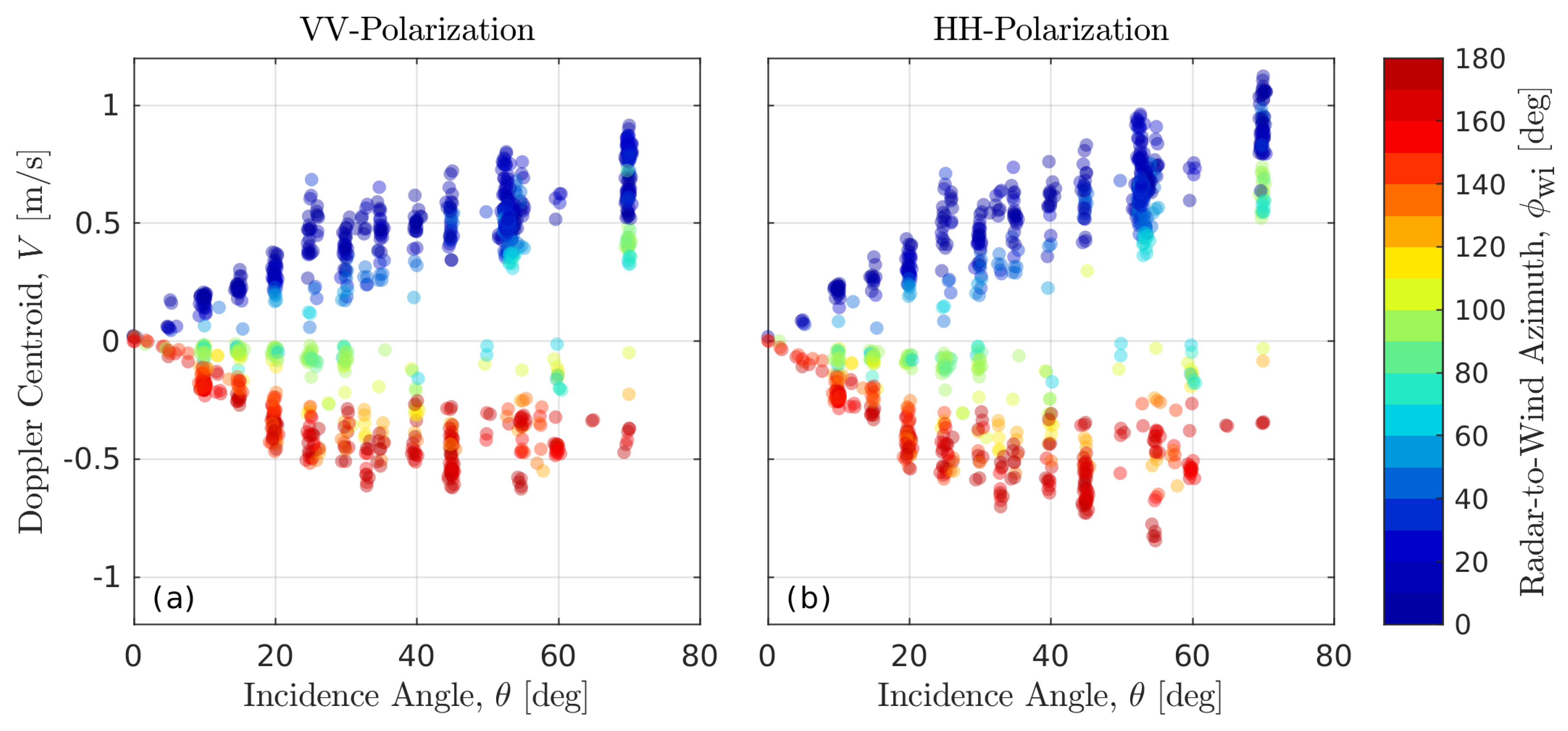
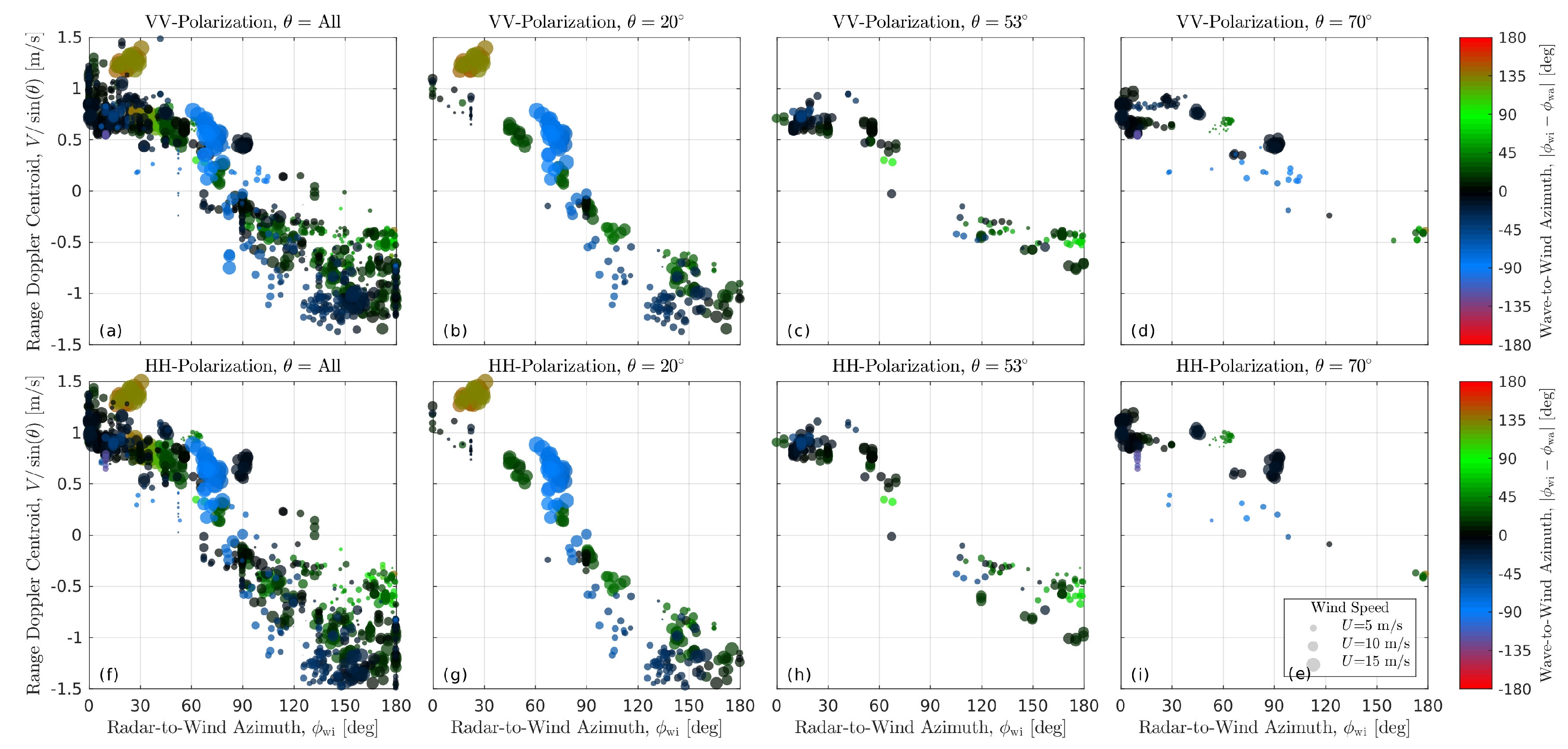
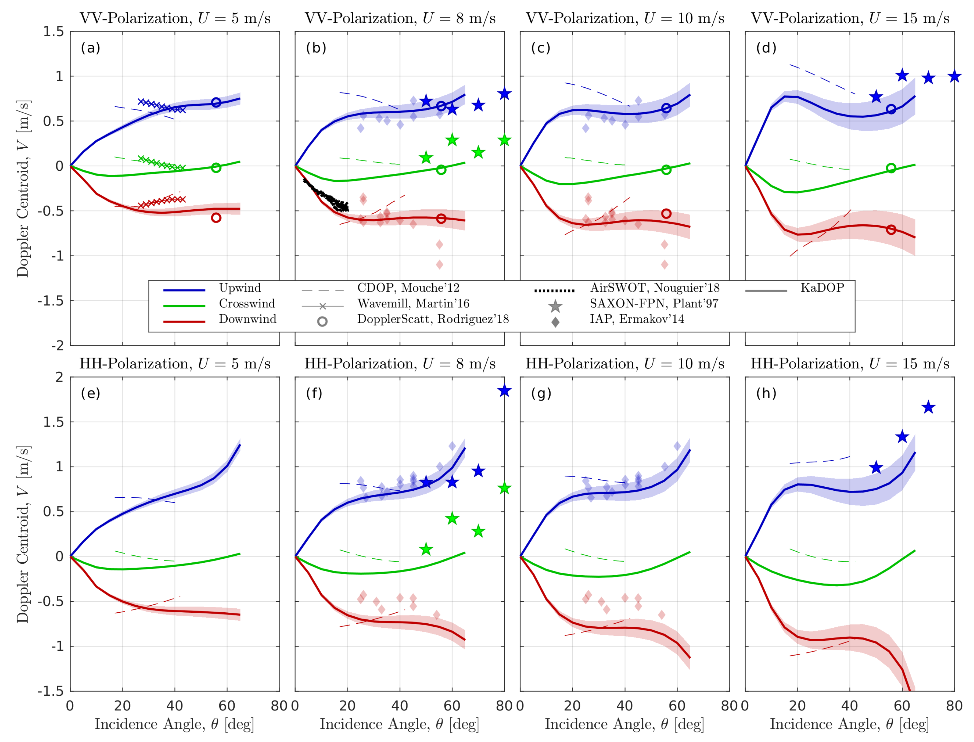
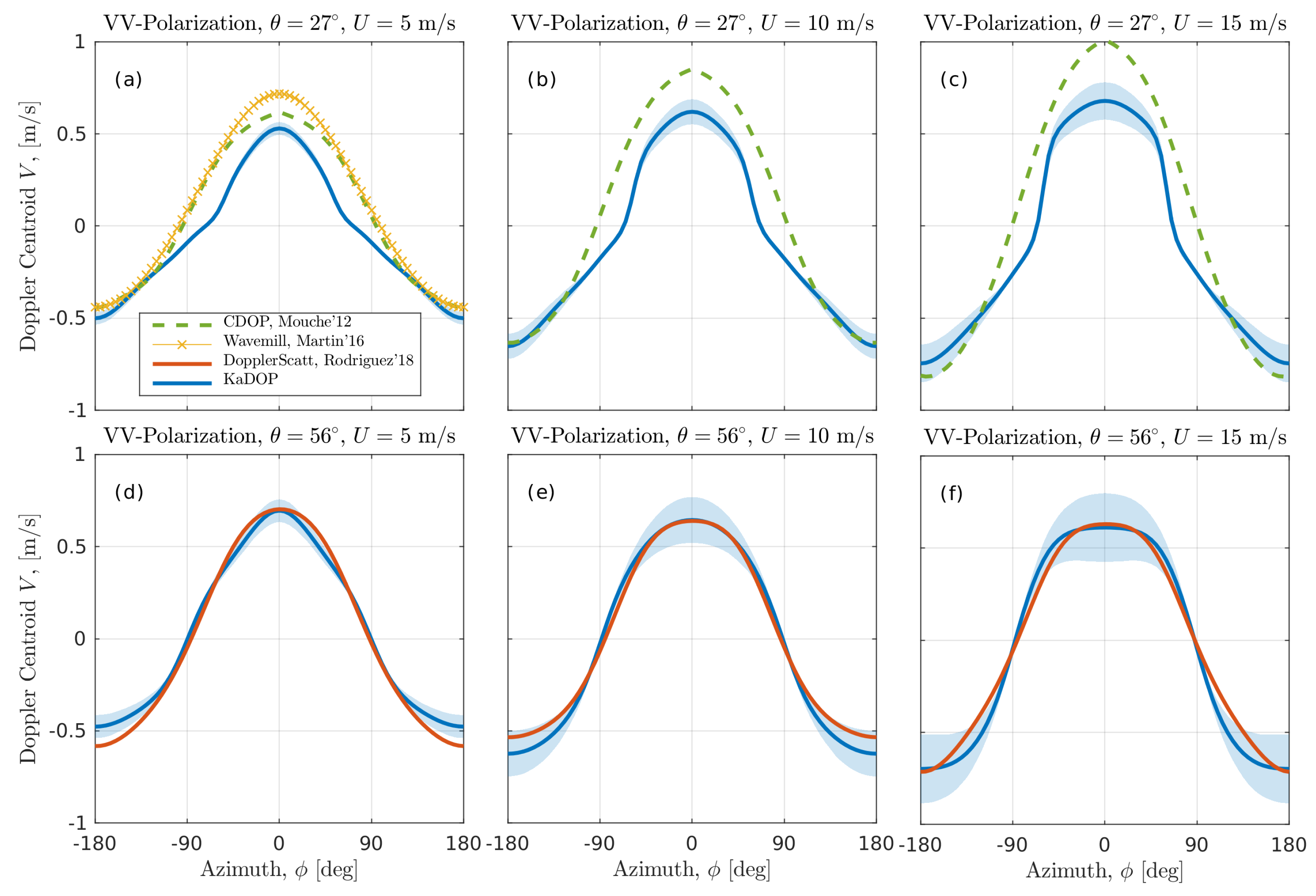
3.1. Look Geometry Dependence

Generally, the variability of measured DC was primarily determined by the radar azimuth, i.e., approaching/passing waves cause positive/negative Doppler shifts, respectively (Figure 3). The magnitude of azimuth variation was determined by the incidence angle and the sea state. Upwind and downwind DC values were approximately the same in magnitude at small $\theta$, but become different at larger $\theta$ (upwind magnitude is larger), especially at HH polarization. Maximal observed DC was ≈1/1.2 m/s at VV/HH polarization at $\theta ={70}^{\circ }$ in the upwind direction.

In the crosswind direction, the DC was unexpectedly non-zero (green symbols in Figure 3): at small $\theta <30$–${40}^{\circ }$, the crosswind DC was systematically negative $V\approx -$0.05–0.1 m/s while, at large $\theta >{60}^{\circ }$, it approached positive values close to those observed in the near-upwind direction, $V\approx$ 0.45–0.65 m/s.

In contrast with Figure 3, which shows only nearly co-aligned winds and waves ($|{\varphi }_{\mathrm{wi}}-{\varphi }_{\mathrm{wa}}|<{25}^{\circ }$, where ${\varphi }_{\mathrm{wi}}$ and ${\varphi }_{\mathrm{wa}}$ are the radar-to-wind and radar-to-wave azimuth, respectively) to outline the incidence angle behavior of the DC, Figure 4 illustrates azimuth DC dependencies as a function of radar-to-wind direction for all observed wind-wave situations. To first order, the data followed a regular, cosine-like dependency for co-aligned winds and waves (black symbols). For differing wind and wave directions, the DC points stand out of the regular dependency, indicating that the DC is a complex function of both wind and wave directions. Figure 4a,b confirm that crosswind DC is somewhat negative at small incidence angles, $\theta ={20}^{\circ }$, while it becomes positive (even for co-aligned wind and waves) at $\theta ={70}^{\circ }$.

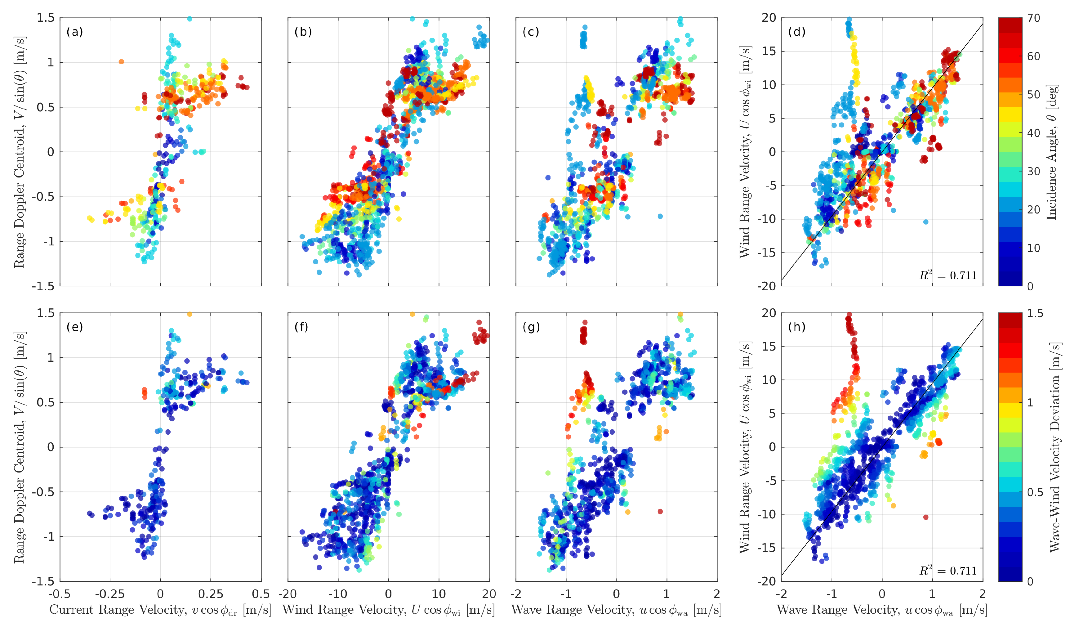
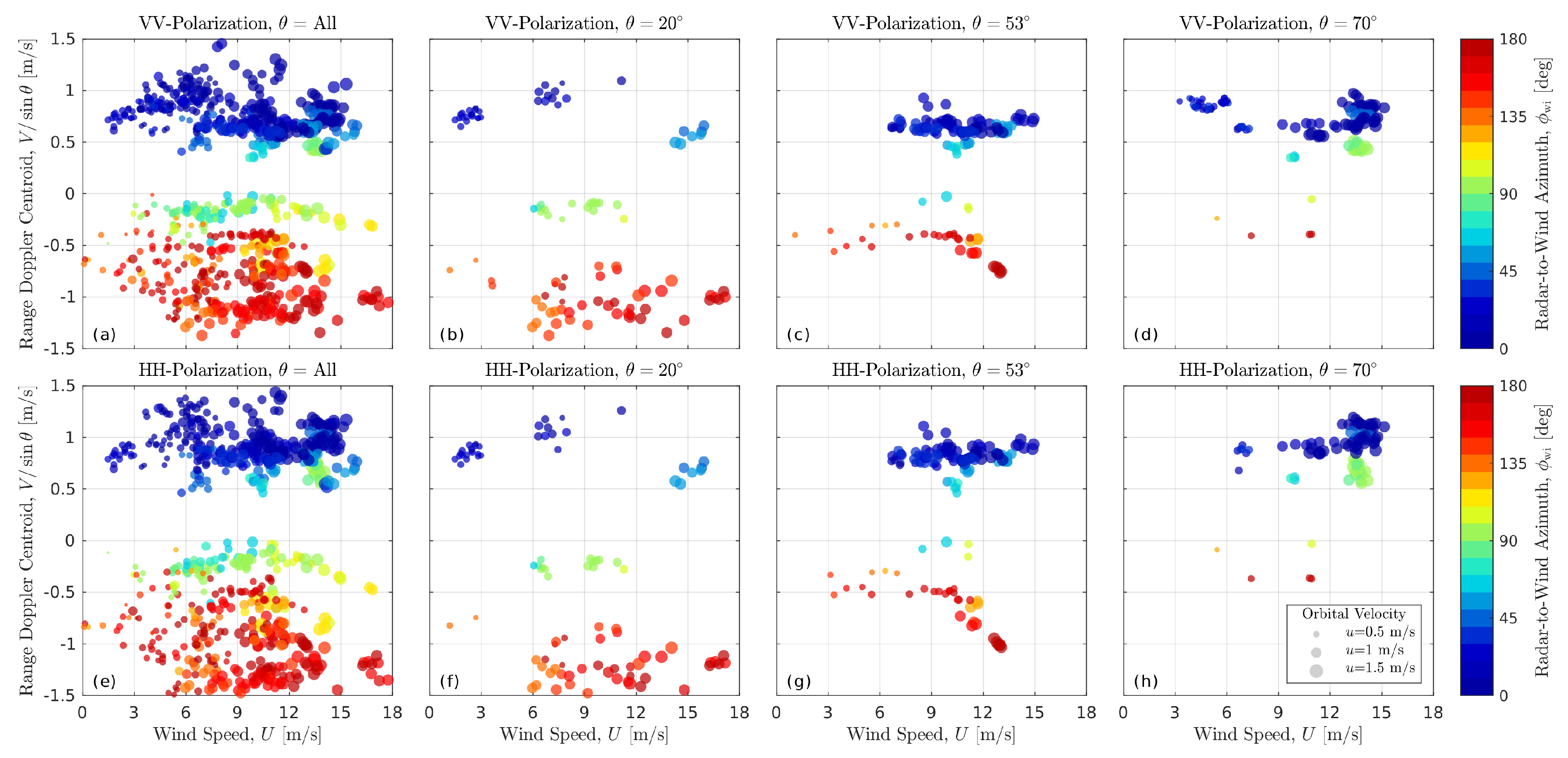
3.2. Sea State Dependence

Previous studies have shown an apparent DC dependence on the wind speed for C-band measurements at $\theta ={40}^{\circ }$ [14], and much less pronounced for Ka-band at $\theta ={56}^{\circ }$ for wind speeds $U=$ 4–12 m/s [21]. Plotting our measurements against wind velocity projected on the radar look direction indicates a clear dependence on the sea state (Figure 5). Only VV data are shown, as HH data look similar. The DC sensitivity to the sea surface current is remarkably dependent on the incidence angle (indicated by colors in Figure 5a). Although the DC followed the sea surface current, a positive/negative bias for upwind/downwind direction, respectively, is also present. Its magnitude increased with decreasing incidence angle. This bias is to be attributed to the wave-induced DC contribution. It is demonstrated more clearly by Figure 5b,c, showing DC dependency on wind speed and characteristic magnitude of wave orbital velocity projection on the the radar incidence plane. Note that $u={\omega }_{\mathrm{p}}{H}_{\mathrm{s}}$ was used as a characteristic magnitude of wave orbital velocity, where ${\omega }_{\mathrm{p}}$ is the wave peak frequency, and $H_{\mathrm{s}}$ is the significant wave height. Hereafter this projection, $ucos{\varphi }_{\mathrm{wa}}$, is referred to as “wave range velocity”. The scatter in these plots was caused by (i) $\theta$ dependence of the wave-induced contribution, (ii) differences between wave and wind azimuths. This is revealed by bottom panels in Figure 5 showing the same data clouds as in the top panels, but color-scaled versus the deviation between wind and wave range velocity components. Like for waves, the wind range velocity is defined as the projection of wind velocity on the radar incidence plane, $Ucos{\varphi }_{\mathrm{wi}}$. As a measure of the above deviation, the distance (along wave range x-axis) between an individual data point and a linear fit to the whole data cloud was used (Figure 5h). It is clearly seen in Figure 5f,g that strong deviations of the DC from its regular wind/wave behavior are coincident with strong deviations between wind and wave range velocity components.

At first glance, the comparison in Figure 5 confirms the presence of sea state dependent DC with magnitudes close to those predicted by CDOP [14]. In fact, the DC was governed by the range projection of wind/wave velocity, ∼$cos\varphi$, rather than the velocity magnitude. This is highlighted in Figure 6, showing the DC as a function of wind speed, U, for various azimuths (specified by different colors). In line with the DopplerScatt observations [21], no significant wind dependency can be detected in Figure 6.

The main objective of this study is to present our Ka-band platform observations in an easy usable form. Normally, e.g., for NRCS analysis, this is achieved by fitting observation data as a function of look geometry and environmental variables, also known as the GMF. As discussed in the above data overview, a plain polynomial fit based solely on the look geometry parameters (such as incidence angle, azimuth) cannot be effectively applied because, among others, the fitting function should involve the sea state parameters. In general, all environmental parameters, including wind speed and direction, significant (dominant) wave height, period and direction should be accounted for. But given the data sparsity, a fit to a large number of variables cannot be well constrained. Thus, for practical purposes, a semi-empirical approach is adopted instead of purely empirical GMF. It is based on a functional form of the sea surface radar echo suggested by a theoretical model (DopRIM [10,11,29]) with scaling parameters fitted by our observations. Below, the DopRIM is briefly described. It is further simplified based on observed Doppler signal properties, available wave parameterizations, and environmental condition limitations of our platform measurements. The DC measurements presented above are used for validations of the proposed semi-empirical model.

4. Model

4.1. Background (DopRIM Approach)

Our approach follows the Doppler radar imaging model (DopRIM) [10,11,29]. It accounts for small-scale waves corresponding to individual scatterers, modulated by large-scale tilting waves. The sea surface DC is an equivalent current, $V=\pi f_{\mathrm{D}}/k_{\mathrm{r}}$, corresponding to the Doppler frequency shift, $f_{\mathrm{D}}$, averaged over large temporal and/or spatial scales,

$$V=v_{\mathrm{dr}}sin\theta cos{\varphi }_{\mathrm{dr}}+v_{\mathrm{sc}}sin\theta +\overline{{\sigma }^{\prime }u}/\overline{\sigma },$$

(1)

where $v_{\mathrm{dr}}$ is the drift speed, ${\varphi }_{\mathrm{dr}}$ is the radar-to-current azimuth angle, $v_{\mathrm{sc}}$ is the inherent scatter velocity projection on the radar incidence plane, u is the line-of-sight projection of the wave orbital velocity, $\sigma =\overline{\sigma }+{\sigma }^{\prime }$ is the sea surface NRCS, represented as a sum of the mean level and variation, $\theta$ is the incidence angle, $k_{\mathrm{r}}$ is the radar wavenumber.

The first term in Equation (1) describes the sea surface current contribution, and the second one is the mean scatterer velocity relative to the sea surface. The third term describes contribution arising from the correlation between large-scale surface (orbital) velocities and (tilt- and hydro-) modulations of the scatterer NRCS.

In the DopRIM, the DC contribution includes resonant and non-resonant scattering mechanisms, and the total DC reads:

$$V=v_{\mathrm{dr}}sin\theta cos{\varphi }_{\mathrm{dr}}+\sum _{n=1,2,3}{P}_n\left(v_{\mathrm{sc}}sin\theta +\overline{{\sigma }^{\prime }u}/\overline{\sigma }\right),$$

(2)

where n denotes the scattering mechanism ($n=1$—Bragg, $n=2$—quasi-specular reflection from regular non-breaking surface, $n=3$—scattering from breaking waves), $P_n={\sigma }_n/\sum \sigma$ is the partial NRCS contribution by the corresponding mechanism.

At moderate and large incidence angles, $\theta >$20–30${}^{\circ }$, the Bragg-resonant and wave breaking mechanisms both contribute, while, at small $\theta <$ 20–30${}^{\circ }$, quasi-specular reflections dominate. Below we describe all DopRIM contributions separately and consider how they can be simplified.

4.2. Moderate and Large Incidence Angles

The inherent velocity corresponding to the resonant scattering mechanism corresponds to the Bragg wave phase velocity,

$$c_{\mathrm{br}}={(g/k_{\mathrm{br}}+{\gamma }_{\mathrm{w}}{k}_{\mathrm{br}})}^{1/2},$$

(3)

where g is the gravity acceleration, ${\gamma }_{\mathrm{w}}$ is the surface tension, and $k_{\mathrm{br}}=2k_{\mathrm{r}}sin\theta$ is the Bragg wavenumber. The backscattered intensity depends on the Bragg wave spectrum, thus the Bragg scatter velocity also depends on the angular distribution of wave spectrum in the direction towards and away from a radar,

$$v_{\mathrm{sc}}=c_{\mathrm{br}}\frac{B(k_{\mathrm{br}},{\varphi }_{\mathrm{wi}})-B(k_{\mathrm{br}},{\varphi }_{\mathrm{wi}}+\pi )}{B(k_{\mathrm{br}},{\varphi }_{\mathrm{wi}})+B(k_{\mathrm{br}},{\varphi }_{\mathrm{wi}}+\pi )},$$

(4)

where B is the directional curvature spectrum, and ${\varphi }_{\mathrm{wi}}$ is the radar-to-wind azimuth.

In the DopRIM, radar scattering from rough surface patches associated with breaking of waves with wavenumbers $k<\min (k_{\mathrm{wb}},k_{\mathrm{r}}/10)$, where $k_{\mathrm{wb}}=2\pi /0.3$ rad/m, significantly contribute to the surface NRCS. Doppler velocity of breaker-facets is equal to the mean phase velocity, c, of breaking waves weighted with their contribution to the fraction of the sea surface covered by breaking zones:

$$c_{\mathrm{wb}}=\underset{k<k_{\mathrm{wb}}}{\int }c{k}^{-1}\mathrm{\Lambda }(k)\mathrm{d}k/\underset{k<k_{\mathrm{wb}}}{\int }{k}^{-1}\mathrm{\Lambda }(k)\mathrm{d}k,$$

(5)

where $\mathrm{\Lambda }(k)\propto {(u_{*}/c)}^2{k}^{-1}B(k)$ is the Phillips $\mathrm{\Lambda }$-distribution [45] for the total length of breaking crests per unit area associated with wavenumber, k, and wave phase velocity, c, $u_{*}$ is the wind friction velocity. If $B=\mathrm{const}$ then, according to Equation (5), the inherent velocity of breaking facets is $c_{\mathrm{wb}}=2c(k_{\mathrm{wb}})$, or about $c_{\mathrm{wb}}\approx 1.4$ m/s.

However, as found in [40], the observed sea surface Doppler shift does not reveal strong spikes at $\theta <{65}^{\circ }$. Also, wave spectra derived from Doppler velocity agree well with in situ wave gauge spectra. It suggests that, although breakers significantly contribute to spike-like NRCS, their impact on instantaneous Doppler shift is weak. As suggested in [40], enhanced surface roughness patches on crests of breaking waves are “embedded” into the water, and thus their Doppler velocity corresponds to the orbital velocity of breaking waves. Joint analysis of collocated radar/video measurements of Doppler/optical velocity of breakers [46] further revealed that Doppler velocity of breakers is slower than the advance velocity of breakers by a factor of ≈4 (traced by whitecap movement). If one assumes that the 1/4 factor corresponds to the characteristic steepness of breaking waves, then the measured Doppler velocity of breakers corresponds to their orbital velocity. Following, one may conclude that the inherent Doppler velocity of breakers defined by Equation (5) is to be scaled by a factor of 1/4. This gives $c_{\mathrm{wb}}=2c(k_{\mathrm{wb}})/4$ or $c_{\mathrm{wb}}\approx 0.35$ m/s, that is comparable with Bragg phase velocity.

Notice that this $c_{\mathrm{wb}}$ estimate is valid for moderate incidence angles only, $\theta <{65}^{\circ }$. At larger incidence angles, especially at HH polarization, the Doppler shift demonstrates quite different features including strong spikes correlated with breaking wave events [40]. However, this study is limited to moderate incidence angles, $\theta <{65}^{\circ }$, and specific Doppler shift features observed at larger incidence angles are not considered.

The last term in Equation (1) is caused by correlated variations of facet NRCS, ${\sigma }^{\prime }$, with its long wave orbital velocity, u. This so-called wave-induced Doppler velocity can be expressed in terms of a complex modulation transfer function (MTF) [47,48],

$$\begin{array}{ccc}\hfill \overline{{\sigma }^{\prime }u}/\overline{\sigma }& =& \mathrm{Re}\left\{MG\right\}{\mathsf{\Omega }}^3{g}^{-1}{A}^2/2=\mathrm{Re}\left\{MG\right\}C{K}^2{A}^2/2,\hfill \end{array}$$

(6)

$$\begin{array}{ccc}\hfill G& =& cos{\varphi }_{\mathrm{wa}}sin\theta -icos\theta ,\hfill \end{array}$$

(7)

where $\mathsf{\Omega }$ is the long wave angular frequency, C is the long wave phase velocity, G is the geometrical coefficient projecting wave orbital velocity onto the radar line-of-sight, M is the complex MTF consisting of tilt- and hydro-MTF, $M=M_{\mathrm{T}}+M_{\mathrm{H}}=i{M}_{\mathrm{T}}cos{\varphi }_{\mathrm{wa}}+\mathrm{Re}\left\{M_{\mathrm{H}}\right\}+i\mathrm{Im}\left\{M_{\mathrm{H}}\right\}$, and ${\varphi }_{\mathrm{wa}}$ is the radar-to-wave azimuth angle.

In the DopRIM, the tilt and hydro-MTF are evaluated separately for Bragg and wave breaking scattering mechanisms (see details in [29,49,50]). Here, we rely on an empirical MTF developed in [40] using the same data set for modulating wave frequency from 0.2 Hz to 0.8 Hz. In contrast to the DopRIM, the empirical MTF combines all mechanisms and there is no need to separate their contributions. Thus, Equation (6) with empirical MTF, M, accounts for both tilt- and hydro-wave-induced contributions of Bragg and wave breaking scattering mechanisms at moderate incidence angles, $\theta >$ 20–30${}^{\circ }$.

4.3. Small Incidence Angles

At small incidence angles, $\theta <$ 20–30${}^{\circ }$, quasi-specular reflections provide dominant contribution to the surface NRCS. The mean Doppler velocity of specular points is derived by Longuet-Higgings [51], and its spectral form is given in [24,29],

$$c_{\mathrm{sp}}=cos{\varphi }_{\mathrm{wi}}{\int }_{L}c{k}^{-2}cos(\varphi )B(\mathbf{k})\mathrm{d}\mathbf{k}/\overline{{\zeta }_{Lup}^2}+sin{\varphi }_{\mathrm{wi}}{\int }_{L}c{k}^{-2}sin(\varphi )B(\mathbf{k})\mathrm{d}\mathbf{k}/\overline{{\zeta }_{Lcr}^2},$$

(8)

where $\varphi$ is the relative to wind azimuth of the spectral component associated with wave vector, $\mathbf{k}$, $[\overline{{\zeta }_{Lup}^2},\overline{{\zeta }_{Lcr}^2}]={\int }_L{k}^{-2}[{cos}^2(\varphi ),{sin}^2(\varphi )]B(\mathbf{k})\mathrm{d}\mathbf{k}$ is the mean square slope (MSS) components of the modulating waves in the upwind and crosswind direction, respectively, and integral in Equation (8) is taken over the large-scale surface waves, i.e., over spectral domain satisfying the condition: $k<k_{\mathrm{r}}/4$.

Equation (8) represents the inherent mean velocity of specular points. However, given a small radar footprint, apparent modulations of NRCS and Doppler velocity by dominant surface waves were observed [40] at low incidence angles. These observations presume that the two-scale concept, with differing scales of waves providing radar backscattered intensity and modulations, can be adopted. This can also be corroborated by the evaluation of integrals in Equation (8). For a characteristic curvature spectrum, $B(k)\approx \mathrm{const}$, the MSS is dominated by the high frequency tail of spectrum, while the integral involving the phase velocity is mainly governed by the low frequency part of the spectrum (dominant waves). Following this concept and using the known NRCS approximation for low incidence angles [24,52,53],

$$\sigma (\theta )\sim {sec}^4\theta exp\left(-\frac{{tan}^2\theta }{2\overline{{\zeta }_{Lup}^2}\overline{{\zeta }_{Lcr}^2}}[\overline{{\zeta }_{Lcr}^2}{cos}^2{\varphi }_{\mathrm{wi}}+\overline{{\zeta }_{Lup}^2}{sin}^2{\varphi }_{\mathrm{wi}}]\right),$$

(9)

along with the definition of tilt-MTF,

$$M_{\mathrm{T}}=\frac{\partial ln\sigma }{\partial tan\theta }=tan\theta \left(\frac{{cos}^2{\varphi }_{\mathrm{wi}}}{\overline{{\zeta }_{Lup}^2}}+\frac{{sin}^2{\varphi }_{\mathrm{wi}}}{\overline{{\zeta }_{Lcr}^2}}\right),$$

(10)

Equation (8) is rewritten for a single dominant long wave as,

$$c_{\mathrm{sp}}sin\theta =\mathrm{Re}\left\{MG\right\}C{K}^2{A}^2/2,$$

(11)

which takes a form similar to Equation (6) describing the wave-induced Doppler velocity. Such similarity is not that surprising. Equation (8) describes the mean velocity of specular points, resulting from the linear superposition of random waves of different scales [51]. The majority of specular points is linked to large local slopes of short scale waves, which are advected by fast, but small slope, dominant surface waves. As such, the mean specular point velocity is linked to parameters describing these dominant waves, as predicted by Equation (11).

4.4. The Semi-Empirical Model

The similarity between Doppler velocity relationships at low, Equation (11), and moderate, Equation (6), incidence angles helps suggest a more unified relationship, valid for all incidence angles. This is especially tempting because the empirical MTF developed in [40] applies to all incidence angles and accounts for all mechanisms responsible for radar backscattering, including quasi-specular reflections at low incidence angles, and Bragg/non-Bragg scattering at larger incidence angles.

First, the inherent Doppler velocity of Bragg waves and breakers can be merged. As discussed above, the inherent velocity of breakers (about 0.35 m/s) is close to the Bragg wave phase velocity. At moderate incidence angles, the sum of weights for Bragg and breaking mechanisms is close to 1. For the sake of simplicity, the Bragg phase velocity is used as a measure of the inherent scatterer velocity, Equation (4), which is evaluated using the angular distribution of Bragg wave spectrum reported in [54] and represented here as,

$$B(k_{\mathrm{br}},{\varphi }_{\mathrm{wi}})\sim {\mathrm{sech}}^2{\varphi }_{\mathrm{wi}}.$$

(12)

The Bragg scatter velocity, Equation (4), is not valid at small $\theta$ where quasi-specular reflection dominates. However, since line-of-sight projection of Bragg velocity tends to zero at $\theta \to 0$ due to $sin\theta$-factor, we assume that Equations (3), (4), and (12) determine the inherent scatterer velocity in the whole range of $\theta$ in our model.

Combining Equations (11) and (6), the unified expression for semi-empirical DC model (KaDOP) valid from small to moderate incidence angles, $\theta <{65}^{\circ }$, reads:

$$V=v_{\mathrm{dr}}sin\theta cos{\varphi }_{\mathrm{dr}}+v_{\mathrm{sc}}sin\theta +{\int }_L\mathrm{Re}\left\{MG\right\}c{k}^{-2}B(\mathbf{k})\mathrm{d}\mathbf{k},$$

(13)

or in terms of directional frequency spectrum, $S(\omega ,\varphi )$,

$$V=v_{\mathrm{dr}}sin\theta cos{\varphi }_{\mathrm{dr}}+v_{\mathrm{sc}}sin\theta +g^{-1}\underset{0}{\overset{2\pi }{\int }}\mathrm{Re}\left\{M(\theta ,\varphi ,U)G(\theta ,\varphi )\right\}\underset{L}{\int }{\omega }^{3}S(\omega ,\varphi )\mathrm{d}\omega \mathrm{d}\varphi .$$

(14)

The frequency integral in Equation (14) is defined by the low-frequency part of the spectrum and thus not sensitive to the upper limit of integration. The empirical MTF developed in [40] is an essential component of this model. Notice that this MTF was originally developed for wave frequencies 0.2–0.8 Hz, and strictly speaking, does not apply to lower frequencies, <0.2 Hz. However, in the absence of a better alternative, we will use it for DC estimates even for wave frequencies out of the MTF validity range.

The third spectrum moment can be evaluated as:

$$\underset{L}{\int }{\omega }^{3}S(\omega )\mathrm{d}\omega \approx \beta ·H_{\mathrm{s}}^2{\omega }_{\mathrm{p}}^3,$$

(15)

For practical applications, when several, N, wave systems are present (mixed sea), Equation (14) can be reduced to

$$V=v_{\mathrm{dr}}sin\theta cos{\varphi }_{\mathrm{dr}}+v_{\mathrm{sc}}sin\theta +g^{-1}\sum _N{\beta }_N·\mathrm{Re}\left\{M(\theta ,{\varphi }_{\mathrm{wa}N},U)G\right\}{H}_{\mathrm{s}N}^2{\omega }_{\mathrm{p}N}^3,$$

(16)

where N is the number of wave systems, $v_{\mathrm{dr}},{\varphi }_{\mathrm{dr}}$ are the sea surface current speed and direction, respectively, $v_{\mathrm{sc}}$ is the inherent scatterer velocity determined by Equations (3), (4) and (12), ${\varphi }_{\mathrm{wa}N}$ is the radar-to-Nth-wave-system direction, U is the 10 m-wind speed, $H_{\mathrm{s}N}$ and ${\omega }_{\mathrm{p}N}$ are the significant wave height (SWH) and peak frequency of the N-th wave system, G is the geometrical coefficient determined by Equation (7), $M(\theta ,{\varphi }_{\mathrm{wa}N},U)$ is the empirical MTF [40] (see also Appendix A).

The coefficient, ${\beta }_N$, in Equation (16) depends on the shape of the frequency spectrum and thus differs for broad wind wave spectrum and narrow swell spectrum. As a first guess, it is estimated from the Pierson-Moskowitz spectrum [55], for which ${\beta }_{\mathrm{ws}}\approx 0.2$. For very narrow (delta-function type) swell spectrum, ${\beta }_{\mathrm{sw}}=1/16$.

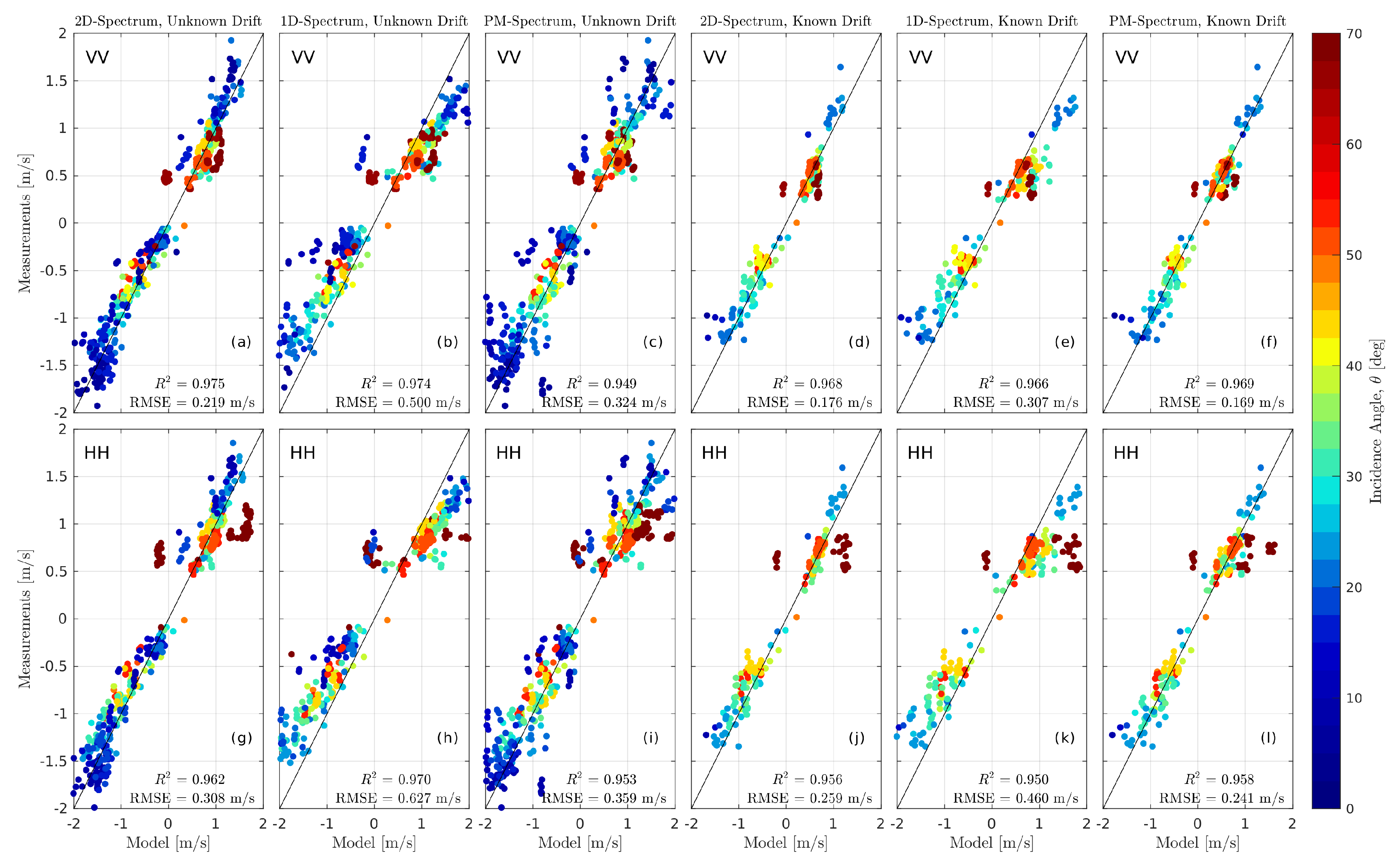
4.5. Model Validation

To validate the KaDOP model, Equation (14), it was first applied to the data subset with known wind and wave conditions, but unknown surface currents (Figure 7, left three columns). As a proxy for 10-m current shear, $1.5\%\mathbf{U}$ was used that was half of the “classical” $3\%\mathbf{U}$ but close to $1.3\%\mathbf{U}$ dependence observed at the platform site [56]. In order to emphasize the importance of angular spreading of wave spectrum on DC, we performed simulations with both, 2D and 1D wave spectra obtained from wave gauge measurements. For the latter case, the directional spectrum $S(\omega ,\varphi )$ was replaced by the omni-directional one, the MTF was specified for the mean wave-direction, and the integration over azimuth was omitted. Further, simulations with 2D/1D spectrum are referred to as KaDOP-2D/KaDOP-1D, respectively.

The KaDOP-2D worked better than the KaDOP-1D which systematically overestimated the measured DC. This is explained by unrealistically narrow azimuth distribution with all the wave energy coming in the same direction, ${\varphi }_{\mathrm{wa}}$. In the 2D case, the real azimuthal distribution was accounted for, to enable a better DC simulation.

At small incidence angles, the range DC as well as its errors are “amplified” by the $1/sin\theta$ factor that leads to larger data scatter. At moderate to large $\theta$, the empirical model works better than at small $\theta$ except at $\theta >$65–70${}^{\circ }$ where the model exhibits significant variability while the measurements do not. This scatter is more pronounced at HH polarization. This is explained by the breaking wave contribution that is indirectly accounted for through the linear empirical MTF. The increased model scatter at large $\theta$ suggests that the concept of linear MTF is applicable only for $\theta <$ 65–70${}^{\circ }$. At larger $\theta$ with large NRCS modulation magnitudes, the linear MTF approximation is no longer accurate [41]. However, we leave this issue out of the scope of this study by limiting the applicability of the KaDOP to small and moderate incidence angles, $\theta <$ 65${}^{\circ }$.

The subset with known drift currents (Figure 7, right three columns) demonstrates similar behavior but with a smaller root-mean-square error. Note that the model is sensitive to the angular width of the wave spectrum (compare Figure 7d,j,e,k light blue points). But, 2D wave spectra were evaluated indirectly from wave gauge records. Data shown above are based on the maximum likelihood method. Application of an alternative maximum entropy method yielded similar spectra but with a narrower angular width of spectrum peak. Thus, uncertainties in wave spectrum estimation also contributed to the uncertainties of the empirical model.

Overall, the correlation coefficient between the KaDOP and measurements (>0.9) was high at $\theta <$ 65–70${}^{\circ }$ that allows extrapolating the KaDOP on an arbitrary wave spectrum. The KaDOP evaluated using Pierson–Moskowitz spectral shape, Equation (16), are shown in Figure 7c,f,i,l. Comparing these simulations with KaDOP-1D simulations (Figure 7b,e,h,k) one may conclude that they are very similar. This fact indicates that the simplified DC model based on observed SWH and spectral peak frequency had similar skill as more complex model utilizing measured wave spectra. For further discussions, Equation (16) is used with wave input parameters expressed in terms of SWH and ${\omega }_p$.

5. Discussion

In this section, we compare the KaDOP with available measurements in different bands:

• Ku-band, data from the FPN-SAXON experiment in the North Sea, VV and HH polarizations, $\theta =$ 50, 60, 70, 80${}^{\circ }$, upwind and crosswind azimuth with co-aligned winds and waves, wind speed $U=7,8,16$ m/s. Doppler spectra from Figures 1–3 in [32] are digitized manually and integrated to obtain the DC.
• C-band, global Advanced SAR data generalized in the CDOP GMF [14], VV and HH polarization, $\theta =$ 17–42${}^{\circ }$, $U=$ 1–17 m/s, all azimuths.
• X-band, measurements by the Institute of Applied Physics RAS (IAP) at the Black Sea research platform (the same place as our data) [33] (their Figure 4b,d), VV and HH polarization, $\theta =$ 25–55${}^{\circ }$, $U=$ 7–14 m/s (wind speed classification is unknown), upwind and downwind azimuths.
• X-band, Wavemill data collected in the Irish Sea [35] (their Table 1), VV polarization $\theta =$ 27–43${}^{\circ }$, all azimuths, mixed sea with $U=5.5$ m/s and swell oblique to the wind direction, swell wavelength $\lambda =50$ m.
• Ka-band, AirSWOT campaign data collected in the Gulf of Mexico [19] (their Figure 16c), VV polarization, $\theta =$ 0–23${}^{\circ }$, downwave/wind azimuth, $U=8$ m/s, peak wavelength $\lambda =45$ m.
• Ka-band, DopplerScatt measurements along the West Coast of North America and in the Gulf of Mexico [21], VV polarization, $\theta ={56}^{\circ }$, all azimuths, $U=$3–15 m/s.

To conduct calculations, the drift current is assumed to vary from 0 to 3% with the mean value of 1.5% of the wind speed. Bragg wave phase speed was set to its characteristic value in the Ka-band, ≈0.35 m/s at moderate incidence angles, which is close to values in the C/X/Ku-bands, ≈0.23–0.26 m/s. As a wave input to the KaDOP, the classical Pierson–Moskowitz relationships for a fully developed sea [55] are used,

$$\begin{array}{ccc}\hfill {\omega }_p& =& 0.83\mathrm{g}/U,\hfill \end{array}$$

(17)

$$\begin{array}{ccc}\hfill \frac{g{H}_{\mathrm{s}}}{U^2}& =& 0.22.\hfill \end{array}$$

(18)

For simplicity, it is assumed that waves propagate in the wind direction, thus radar-to-wind and radar-to-wave azimuths are the same, ${\varphi }_{\mathrm{wi}}={\varphi }_{\mathrm{wa}}=\varphi$.

5.1. Look Geometry Dependence

In general, the KaDOP, Equation (16), reproduces fairly well all independent observations, but the CDOP that is somewhat underestimated (Figure 8). The DC at HH polarization is remarkably higher than at VV polarization in line with the dual-polarized SAXON-FPN, IAP and CDOP data. The IAP data are in good agreement with KaDOP except for downwind HH polarization. Note that in the KaDOP, the polarization sensitivity is determined by the MTF polarization dependence only. The AirSWOT is somewhat overestimated, probably due to the fact that a full-developed Pierson–Moskowitz spectrum is not exactly the case for fetch limited AirSWOT waves. The same applies to the Wavemill which is based on complicated mixed sea conditions.

The sign of crosswind DC discussed earlier in the raw data analysis (Figure 4) is also reproduced by the KaDOP. The crosswind DC zeros at $\theta \approx {60}^{\circ }$ in line with the DopplerScatt at $\theta ={56}^{\circ }$. In contrast with the KaDOP, the CDOP and Wavemill models predict small but positive crosswind DC at moderate $\theta =20$–${40}^{\circ }$. This is also demonstrated by azimuth dependencies of KaDOP DC (Figure 9) that better agree with the DopplerScatt than with the CDOP and Wavemill.

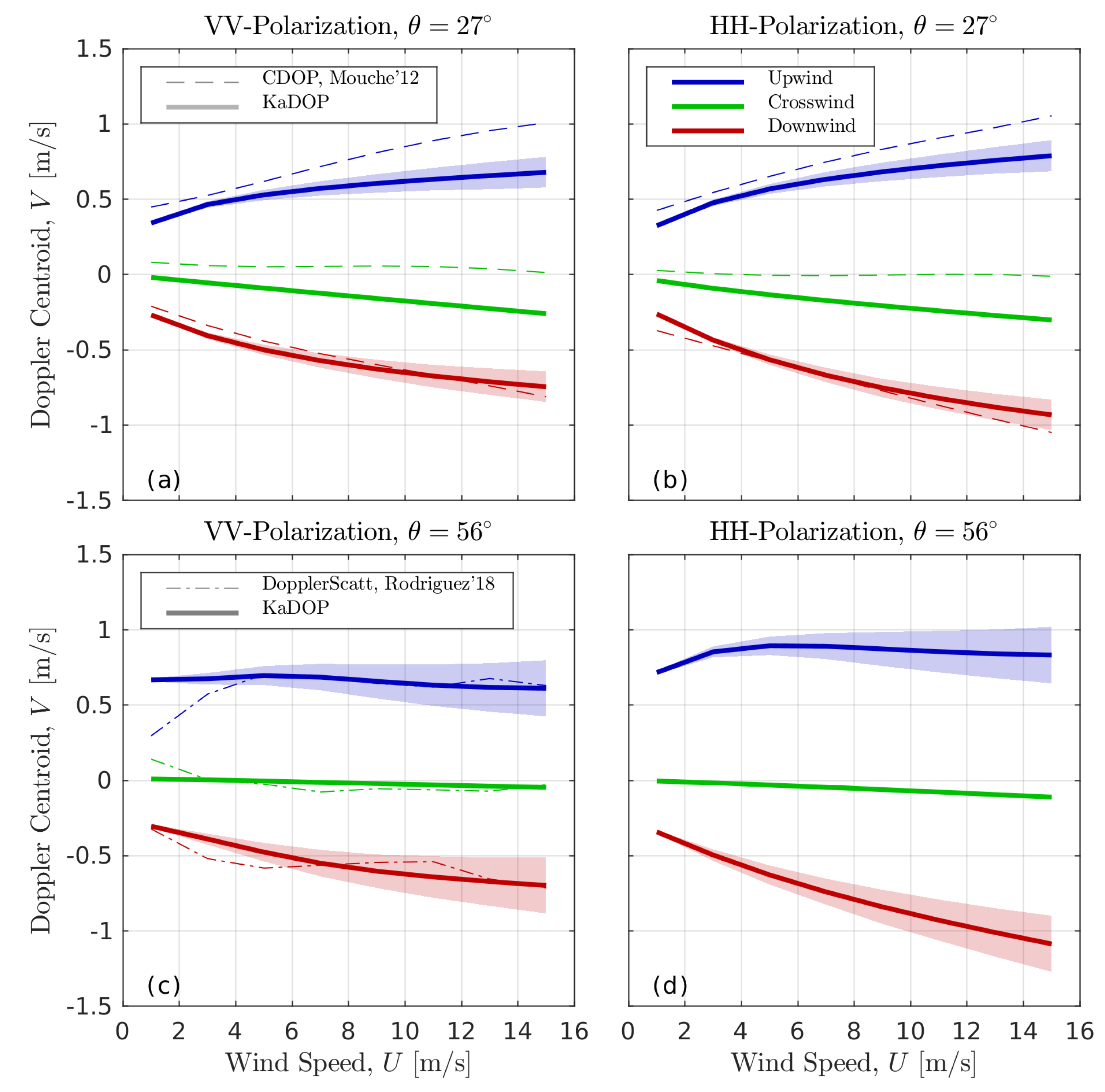
5.2. Wind Speed Dependence

KaDOP wind speed dependence of the DC is generally consistent with the DopplerScatt and CDOP, except for the CDOP in the upwind direction (Figure 10). The difference between DC wind speed dependencies at different incidence angles can be explained by the balance between orbital velocity and MTF magnitudes that differently respond to the wind speed. For an omni-directional elevation ${\omega }^{-5}$-spectrum, the magnitude of orbital velocity, $u=a\omega$, is inversely proportional to wave frequency, $u\sim {\omega }^{-1.5}$. For a given wave age, $U/c_{\mathrm{p}}=\mathrm{const}$, the magnitude of orbital velocity is approximately a linear function of wind speed, $u\sim U^{1.5}$. On the other hand, the MTF increases with wind speed decreasing. To the first order, the tilt-MTF is inversely proportional to the MSS, $M_{\mathrm{T}}=\partial ln\sigma /\partial \theta \sim 1/\overline{{\zeta }^2}$, that in turn linearly increases with U. But, the contribution of hydrodynamic modulations makes the total MTF a more complex function of wind speed. Thus, the DC wind speed dependence is determined by relative changes of magnitudes of orbital velocity and MTF. In addition, it also depends on the wind drift velocity, which is also a linear function of $Usin\theta$.

5.3. Upwind/Downwind Asymmetry

There exists a slight but important difference between DC magnitudes in the upwind and downwind directions, an upwind/downwind asymmetry (UDA), $\mathrm{UDA}=|V_{\mathrm{up}}|/|V_{\mathrm{down}}|$. It is attributed to the hydrodynamics modulation that impacts the DC in opposite ways for upwind and downwind look directions. This effect is expected to decrease with wind speed following the related decrease in the magnitude of hydro-MTF. There are noticeable differences in UDA behavior for different empirical models (Figure 11). In the CDOP, the difference between upwind and downwind DC is always positive and the UDA is about 0.2–0.4 higher at VV than at HH polarization. In contrast, the KaDOP does not show such strong UDA polarization difference. At $\theta ={56}^{\circ }$, KaDOP UDA decreases with increasing wind speed from $\approx 1.3$–$1.4$ at $U=5$ m/s to $\approx 0.8$–$0.9$ at $U=15$ m/s in line with the DopplerScatt. The latter $\mathrm{UDA}<1$ values indicate that the magnitude of downwind DC exceeds the magnitude of upwind DC. Such behavior is explained by the impact of hydrodynamics modulation that changes its phase depending on wind speed (see e.g., Figure 11d in [40]). At moderate winds, $U=7$ m/s, the peak of hydro-MTF locates on crests/forward slopes of long modulating waves but shifts on rear slopes at stronger winds, $U>10$ m/s.

5.4. Crosswind Doppler Centroid

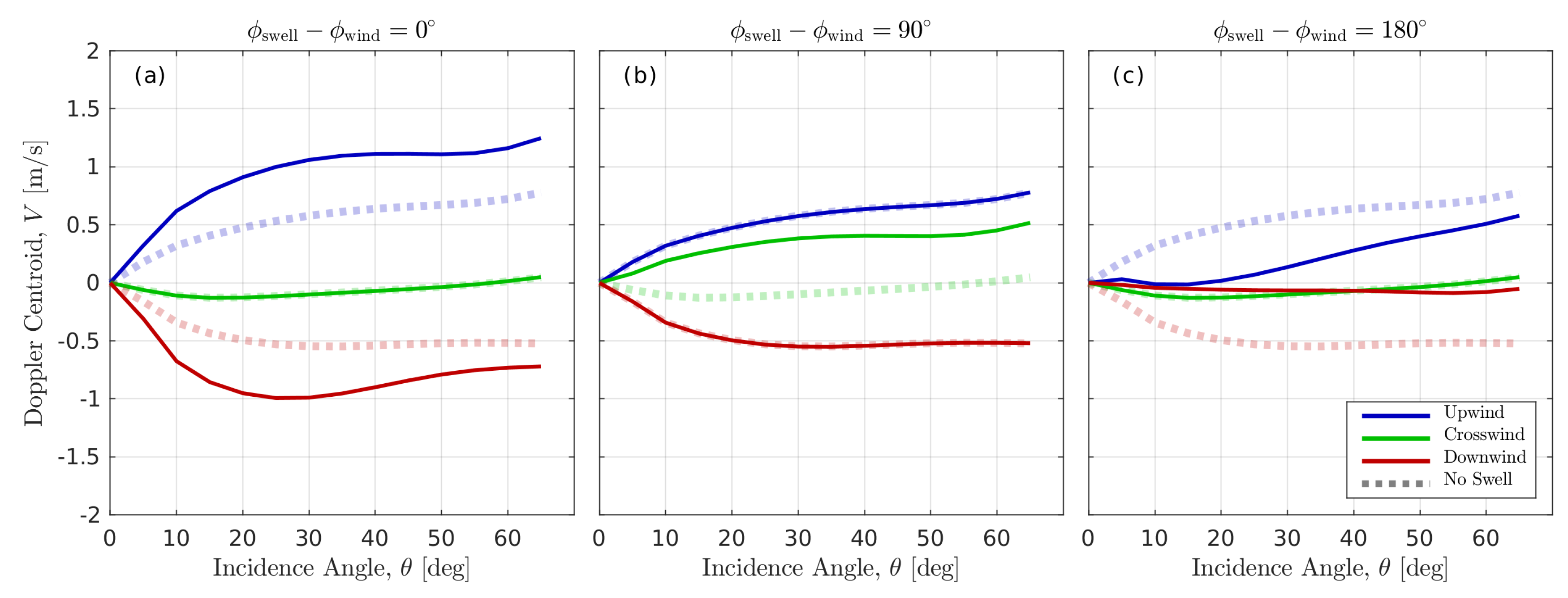
One of the most challenging KaDOP features is its non-zero crosswind behavior. Crosswind KaDOP DC is remarkably negative for $\theta <{60}^{\circ }$. In contrast, CDOP and Wavemill crosswind DC is about zero in this range of $\theta$. This discrepancy may be interpreted in the following way.

Crosswind DC (its sign and magnitude) is controlled by phase and magnitude of the hydro-MTF (impact of crosswind tilt-MTF is zero). The empirical MTF, which is the component of the suggested KaDOP model, predicts the shift of the backscattering modulation peak on the windward (rear) slope of modulating waves, that leads (as follows from Equation (16)) to negative crosswind DC. As discussed in [40,57], the observed shift of modulation peak on the windward wave slope results from wave-induced airflow acceleration over windward wave slopes. This effect occurs only for developing wind waves for which the shift of maximum wind velocity on the rear slope is directly related to the appearance of positive air pressure anomaly over the leeward wave slope, the pressure anomaly that provides energy transfer from wind to waves. Thus, the shift of small-scale surface roughness onto the windward wave slope is a very natural phenomenon, which is, nevertheless, present if (and only if) these dominant wind waves are rather young. This is typical for the Black Sea platform observations characterized by fetch-limited conditions. A similar Ka-band MTF phase behavior was found in the SAXON-FPN measurements at $\theta ={45}^{\circ }$ [58] (see their Figure 4) conducted from an offshore platform in the North Sea.

When wind waves are fully developed, wave-induced wind undulations almost vanish over dominant waves (at least, because the wave phase velocity is close to wind speed). In this case, there is no mechanism which could shift the backscattering modulation peak onto the windward slope. As a consequence, the crosswind DC should be about zero. In case of a swell, swell-induced wind acceleration occurs either over wave crests or in wave troughs depending on the relative wind-swell propagation direction [59,60]. Thus, a swell does not produce a shift of aerodynamic modulations on either of swell wave slopes. In case of a swell, we should not expect the appearance of slope correlated component of hydro-MTF which could contribute to the crosswind DC.

Overall, the observed negative crosswind DC can be most plausibly attributed to the young wind sea effect. This type of waves is typical for coastal platform measurements and, therefore, is a specific feature of our empirical MTF, $M_{\mathrm{ws}}$ (with “ws” standing for wind sea). This empirical MTF predicts a shift of hydro-MTF to the rear slope of the modulating wave. But, it should not probably be extrapolated to open ocean conditions where fully developed sea and swell are much more typical. Such specific limitation of the $M_{\mathrm{ws}}$ can easily be fixed (to the first order) by its modification via forcing the crosswind MTF phase to zero (see Appendix A for details). We suggest using this modified MTF, $M_{\mathrm{sw}}$ (with “sw” standing for swell), for applications of the KaDOP model in open ocean conditions.

5.5. Swell Impact

In the open ocean, swell waves may have extremely long wavelength and phase speed, $C_{\mathrm{sw}}\approx 30$ m/s. Having only very small steepness, ${(AK)}_{\mathrm{sw}}=$ 0.01–0.05, these waves, nevertheless, induce orbital motions with magnitudes, $C_{\mathrm{sw}}{(AK)}_{\mathrm{sw}}=$ 0.3–1.5 m/s, which may be of the order of wind-wave-induced DC. Swell may travel thousands of kilometers from its generation source and thus have arbitrary direction relative to the local wind wave direction. The KaDOP, Equation (16) with $M_{\mathrm{ws}}$ and $M_{\mathrm{sw}}$ used for wind sea and swell contributions, allows estimating the possible influence of ocean swell on the DC for various swell-to-wind directions.

As a first guess for possible swell impacts, the mixed sea DC is simulated in Figure 12 using wind sea $M_{\mathrm{ws}}$ at $U=6$ m/s and the Pierson–Moskowitz spectrum. The impact of the swell is added using $M_{\mathrm{sw}}$ for various swell-to-wind azimuths. Parameters of the swell are somewhat exaggerated: ${\lambda }_{\mathrm{sw}}=600$ m, $T_{\mathrm{sw}}=20$ s, ${(AK)}_{\mathrm{sw}}$ = 0.05, $A_{\mathrm{sw}}=5$ m.

For co-aligned wind and swell, the impact of swell increases the magnitude of upwind and downwind DC by $\approx 100\%$ while the crosswind DC remains unchanged, as expected (Figure 12a). The same holds for the case of upwind swell (Figure 12c), but wind sea and swell contributions compensate each other in this case.

Crosswind swell (Figure 12b) does not affect upwind and downwind DC, but dramatically changes the crosswind DC. Depending on the swell direction, either to the left or to the right of the wind, the crosswind DC changes its sign and magnitude. The latter may become comparable to upwind/downwind DC values.

These simulations demonstrate the significant effect a large swell may have on open ocean DC. Thus, partial disagreement of the wind-sea-KaDOP with the CDOP and Wavemill (Figure 8) can be attributed to the effect of mixed sea present in the Wavemill experiment and evidently present in the global ocean CDOP data set.

Notice, this is only a qualitative simulation, in part, because $M_{\mathrm{sw}}$ phase is set to zero in the crosswind direction. In line with discussions in the previous section, it could be noted that more realistic MTF should also include the impact of wave-induced wind stress modulation and the corresponding crest/trough-correlated hydro-MTF which may impact upwave and downwave (relative to the swell) DC estimates.

6. Conclusions

This paper presents measurements of the Doppler spectrum centroid (DC) conducted from the Black Sea research platform in an attempt to systematize the multi-year in situ co-polarized data in a wide range of incidence angles, azimuths, and winds obtained in well controlled sea state (wave) conditions, and provide a model to describe the Doppler characteristics. In contrast with the NRCS, the observed DC is primary dependent on the characteristics of energy containing waves. The DC cannot be fully described in terms of just wind speed like it is usually done for radar cross-section geophysical model functions. It is preferable to use the observed wave spectrum, or its parameterization, rather than the wind-alone as an input parameter to the DC model.

In this work we use a simplified semi-empirical model to fit Ka-band DC data (KaDOP, source codes are available in the Supplementary Materials). It is based on the Doppler Radar Imaging Model (DopRIM, [11,29]) involving two-scale surface decomposition. Further simplifications include the usage of an empirical MTF [40], instead of the theoretical MTF. Empirical MTF naturally includes all mechanisms (tilt, hydro, Bragg, wave breaking) and thus can be used to describe wave-induced DC contribution at moderate incidence angles, $\theta$. At small $\theta$, the mean specular point velocity is determined by the same equation as the wave-induced contribution at moderate $\theta$. Thus, these two terms are combined and the empirical MTF is solely used to model the DC for small to moderate incidence angles. The average wave breaking Doppler velocity, originally considered significant in the DopRIM, is shown to be close to Bragg wave phase velocity due to the effect of embedding (slowing down) of wave breaking scatterers into the water [40,46].

The KaDOP adequately reproduces the measured DC when in situ wave gauge spectra and surface currents are used as model inputs. The only exception is the large incidence angle case, $\theta ={70}^{\circ }$, for which HH polarization model DC is inadequate and clearly indicates missing effects of wave breaking and resulting MTF non-linearity. Thus the KaDOP applicability is limited to $\theta \le {65}^{\circ }$. This limitation allows to keep the issue of wave breaking impact on the DC at large incidence angles out of the scope of the present study.

Based on fairly good KaDOP performance versus the ground truth training data set, we check the effect of substitution of observed wave spectrum by empirical spectrum models. In this approximation, the KaDOP is a function of the peak wave frequency and SWH. With Pierson–Moskowitz parameters [55] as an input, the KaDOP agrees well with the Ka-band DopplerScatt [21] and AirSWOT [19] data, as well as with the Ku-band SAXON-FPN data [32], X-band IAP [33] (except for HH downwind). The C-band CDOP [14] and X-band Wavemill [35] data are systematically underestimated in the upwind direction.

The KaDOP suggests negative DC values in the crosswind look direction (equivalent motion away from an observer) at $\theta <{50}^{\circ }$. Qualitatively, this is explained by the hydrodynamics MTF that peaks on windward wave slopes. Speculatively, this effect reflects an acceleration of air flow above windward slopes of developing waves. Indirectly, this feature is confirmed by independent Ka-band MTF measurements from the SAXON-FPN experiment [58]. These latter data also reveal a negative MTF phase in near-to-crosswind look directions. However, the airflow acceleration is possible only for wind faster than wave (developing wind sea), while for swell-dominated sea, the hydro-MTF is not slope-correlated. As the first guess for the swell-MTF, unavailable from our data, we refit the original wind-sea MTF with crosswind phase forced to zero.

With both wind-sea and swell-MTF, the KaDOP shows a clear impact of swell on the DC measurements. Thus, the disagreement between KaDOP and mixed-sea observations (CDOP and Wavemill), besides differences in microwave bands and corresponding MTF, can be attributed to peculiarities of the real spectrum that can differ from the Pierson–Moskowitz model and can be impacted by a swell.

Overall, the main purpose of this study is to show that proposed simplified semi-empirical approach based on observed MTF and integral parameters of long wave spectrum, is promising. With empirical MTF and a simple Pierson–Moskowitz spectrum, the KaDOP is capable of reproducing most of the available independent data sets. The KaDOP is validated against our Black sea fetch-limited measurements (fetch $<400$ km, wind speed $<15$ m/s, dominant wavelength $<40$ m, SWH $<1.5$ m). Further improvements of DC predictions are tied with better wave spectrum description and MTF parameterization, no matter empirical or theoretical.

References

1. Naderi, F.M.; Freilich, M.H.; Long, D.G. Spaceborne radar measurement of wind velocity over the ocean—An overview of the NSCAT scatterometer system. Proc. IEEE 1991, 79, 850–866. [Google Scholar] [CrossRef]
2. Hauser, D.; Tison, C.; Amiot, T.; Delaye, L.; Corcoral, N.; Castillan, P. SWIM: The First Spaceborne Wave Scatterometer. IEEE Trans. Geosci. Remote Sens. 2017, 55, 3000–3014. [Google Scholar] [CrossRef]
3. Hasselmann, K.; Raney, R.K.; Plant, W.J.; Alpers, W.; Shuchman, R.A.; Lyzenga, D.R.; Rufenach, C.L.; Tucker, M.J. Theory of synthetic aperture radar ocean imaging: A MARSEN view. J. Geophys. Res. (Oceans) 1985, 90, 4659–4686. [Google Scholar] [CrossRef]
4. Chapron, B.; Johnsen, H.; Garello, R. Wave and wind retrieval from sar images of the ocean. Annales Des Télécommunications 2001, 56, 682–699. [Google Scholar]
5. Goldstein, R.M.; Zebker, H.A. Interferometric radar measurement of ocean surface currents. Nature 1987, 328, 707–709. [Google Scholar] [CrossRef]
6. Thompson, D.R.; Jensen, J.R. Synthetic aperture radar interferometry applied to ship-generated internal waves in the 1989 Loch Linnhe experiment. J. Geophys. Res. (Oceans) 1993, 98, 10259–10270. [Google Scholar] [CrossRef]
7. Romeiser, R.; Thompson, D.R. Numerical study on the along-track interferometric radar imaging mechanism of oceanic surface currents. IEEE Trans. Geosci. Remote Sens. 2000, 38, 446–458. [Google Scholar] [CrossRef]
8. Frasier, S.J.; Camps, A.J. Dual-beam interferometry for ocean surface current vector mapping. IEEE Trans. Geosci. Remote Sens. 2001, 39, 401–414. [Google Scholar] [CrossRef] [Green Version]
9. Martin, A.; Gommenginger, C. Towards wide-swath high-resolution mapping of total ocean surface current vectors from space: Airborne proof-of-concept and validation. Remote Sens. Environ. 2017, 197, 58–71. [Google Scholar] [CrossRef] [Green Version]
10. Chapron, B.; Collard, F.; Ardhuin, F. Direct measurements of ocean surface velocity from space: Interpretation and validation. J. Geophys. Res. (Oceans) 2005, 110, 7008. [Google Scholar] [CrossRef]
11. Johannessen, J.A.; Chapron, B.; Collard, F.; Kudryavtsev, V.; Mouche, A.; Akimov, D.; Dagestad, K.F. Direct ocean surface velocity measurements from space: Improved quantitative interpretation of Envisat ASAR observations. Geophys. Res. Lett. 2008, 35, 22608. [Google Scholar] [CrossRef]
12. Hansen, M.W.; Collard, F.; Dagestad, K.; Johannessen, J.A.; Fabry, P.; Chapron, B. Retrieval of Sea Surface Range Velocities From Envisat ASAR Doppler Centroid Measurements. IEEE Trans. Geosci. Remote Sens. 2011, 49, 3582–3592. [Google Scholar] [CrossRef]
13. Johnsen, H.; Nilsen, V.; Engen, G.; Mouche, A.A.; Collard, F. Ocean Doppler anomaly and ocean surface current from Sentinel 1 TOPS mode. In Proceedings of the International Geoscience and Remote Sensing Symposium–IGARSS, Beijing, China, 10–15 July 2016; pp. 3993–3996. [Google Scholar] [CrossRef]
14. Mouche, A.A.; Collard, F.; Chapron, B.; Dagestad, K.F.; Guitton, G.; Johannessen, J.A.; Kerbaol, V.; Hansen, M.W. On the Use of Doppler Shift for Sea Surface Wind Retrieval From SAR. IEEE Trans. Geosci. Remote Sens. 2012, 50, 2901–2909. [Google Scholar] [CrossRef]
15. Alpers, W.; Mouche, A.; Horstmann, J.; Ivanov, A.Y.; Barabanov, V.S. Application of a new algorithm using Doppler information to retrieve complex wind fields over the Black Sea from ENVISAT SAR images. Int. J. Remote Sens. 2015, 36, 863–881. [Google Scholar] [CrossRef]
16. Gommenginger, C.; Chapron, B.; Martin, A.; Marquez, J.; Brownsword, C.; Buck, C. SEASTAR: A new mission for high-resolution imaging of ocean surface current and wind vectors from space. In Proceedings of the European Conference on Synthetic Aperture Radar—EUSAR, Aachen, Germany, 4–7 June 2018; pp. 1433–1436. [Google Scholar]
17. Martin, A.C.H.; Gommenginger, C.P.; Quilfen, Y. Simultaneous ocean surface current and wind vectors retrieval with squinted SAR interferometry: Geophysical inversion and performance assessment. Remote Sens. Environ. 2018, 216, 798–808. [Google Scholar] [CrossRef]
18. Ardhuin, F.; Aksenov, Y.; Benetazzo, A.; Bertino, L.; Brandt, P.; Caubet, E.; Chapron, B.; Collard, F.; Cravatte, S.; Dias, F.; et al. Measuring currents, ice drift, and waves from space: The Sea Surface KInematics Multiscale monitoring (SKIM) concept. Ocean Sci. 2018, 14, 337–354. [Google Scholar] [CrossRef]
19. Nouguier, F.; Chapron, B.; Collard, F.; Mouche, A.; Rascle, N.; Ardhuin, F.; Wu, X. Sea Surface Kinematics From Near-Nadir Radar Measurement. IEEE Trans. Geosci. Remote Sens. 2018, 56, 6169–6179. [Google Scholar] [CrossRef]
20. Bourassa, M.A.; Rodriguez, E.; Chelton, D. Winds and currents mission: Ability to observe mesoscale AIR/SEA coupling. In Proceedings of the International Geoscience and Remote Sensing Symposium–IGARSS, Beijing, China, 10–15 July 2016; pp. 7392–7395. [Google Scholar] [CrossRef]
21. Rodriguez, E.; Wineteer, A.; Perkovic-Martin, D.; Gál, T.; Stiles, B.; Niamsuwan, N.; Rodriguez Monje, R. Estimating Ocean Vector Winds and Currents Using a Ka-Band Pencil-Beam Doppler Scatterometer. Remote Sens. 2018, 10, 576. [Google Scholar] [CrossRef]
22. Zavorotny, V.U.; Voronovich, A.G. Two-scale model and ocean radar Doppler spectra at moderate and low-grazing angles. IEEE Trans. Ant. Propag. 1998, 46, 84–92. [Google Scholar] [CrossRef]
23. Toporkov, J.V.; Brown, G.S. Numerical simulations of scattering from time-varying, randomly rough surfaces. IEEE Trans. Ant. Propag. 2000, 38, 1616–1625. [Google Scholar] [CrossRef]
24. Chapron, B.; Collard, F.; Kerbaol, V. Satellite Synthetic Aperture Radar Sea Surface Doppler Measurements. In Proceedings of the 2nd Workshop on Coastal and Marine Applications of SAR, Svalbard, Norway, 8–12 September 2003; pp. 133–140. [Google Scholar]
25. Mouche, A.A.; Chapron, B.; Reul, N.; Collard, F. Predicted Doppler shifts induced by ocean surface wave displacements using asymptotic electromagnetic wave scattering theories. Waves Rand. Med. 2008, 18, 185–196. [Google Scholar] [CrossRef]
26. Nouguier, F.; Guerin, C.; Soriano, G. Analytical Techniques for the Doppler Signature of Sea Surfaces in the Microwave Regime—I: Linear Surfaces. IEEE Trans. Geosci. Remote Sens. 2011, 49, 4856–4864. [Google Scholar] [CrossRef]
27. Nouguier, F.; Guerin, C.; Soriano, G. Analytical Techniques for the Doppler Signature of Sea Surfaces in the Microwave Regime—II: Nonlinear Surfaces. IEEE Trans. Geosci. Remote Sens. 2011, 49, 4920–4927. [Google Scholar] [CrossRef]
28. Wang, Y.; Zhang, Y.; He, M.; Zhao, C. Doppler Spectra of Microwave Scattering Fields From Nonlinear Oceanic Surface at Moderate- and Low-Grazing Angles. IEEE Trans. Geosci. Remote Sens. 2012, 50, 1104–1116. [Google Scholar] [CrossRef]
29. Hansen, M.W.; Kudryavtsev, V.; Chapron, B.; Johannessen, J.A.; Collard, F.; Dagestad, K.F.; Mouche, A.A. Simulation of radar backscatter and Doppler shifts of wave-current interaction in the presence of strong tidal current. Remote Sens. Environ. 2012, 120, 113–122. [Google Scholar] [CrossRef]
30. Fois, F.; Hoogeboom, P.; Le Chevalier, F.; Stoffelen, A. An analytical model for the description of the full-polarimetric sea surface Doppler signature. J. Geophys. Res. (Oceans) 2015, 120, 988–1015. [Google Scholar] [CrossRef] [Green Version]
31. Plant, W.J.; Alpers, W. An Introduction to SAXON-FPN. J. Geophys. Res. (Oceans) 1994, 99, 9699–9703. [Google Scholar] [CrossRef]
32. Plant, W.J. A model for microwave Doppler sea return at high incidence angles: Bragg scattering from bound, tilted waves. J. Geophys. Res. (Oceans) 1997, 102, 21131–21146. [Google Scholar] [CrossRef] [Green Version]
33. Ermakov, S.A.; Kapustin, I.A.; Kudryavtsev, V.N.; Sergievskaya, I.A.; Shomina, O.V.; Chapron, B.; Yurovskiy, Y.Y. On the Doppler Frequency Shifts of Radar Signals Backscattered from the Sea Surface. Radiophys. Quant. Electron. 2014, 57, 239–250. [Google Scholar] [CrossRef]
34. Ryabkova, M.S.; Karaev, V.Y.; Titchenko, Y.A.; Meshkov, E.M. Experimental study of the microwave radar Doppler spectrum backscattered from the sea surface at low incidence angles. In Proceedings of the 32nd General Assembly and Scientific Symposium of the International Union of Radio Science–URSI GASS, Montreal, ON, Canada, 19–26 August 2017; IEEE: Washington, DC, USA, 2017. [Google Scholar] [CrossRef]
35. Martin, A.C.H.; Gommenginger, C.; Marquez, J.; Doody, S.; Navarro, V.; Buck, C. Wind-wave-induced velocity in ATI SAR ocean surface currents: First experimental evidence from an airborne campaign. J. Geophys. Res. (Oceans) 2016, 121, 1640–1653. [Google Scholar] [CrossRef] [Green Version]
36. Bao, Q.; Lin, M.; Zhang, Y.; Dong, X.; Lang, S.; Gong, P. Ocean Surface Current Inversion Method for a Doppler Scatterometer. IEEE Trans. Geosci. Remote Sens. 2017, 55, 6505–6516. [Google Scholar] [CrossRef]
37. Miao, Y.; Dong, X.; Bao, Q.; Zhu, D. Perspective of a Ku-Ka Dual-Frequency Scatterometer for Simultaneous Wide-Swath Ocean Surface Wind and Current Measurement. Remote Sens. 2018, 10, 1042. [Google Scholar] [CrossRef]
38. Rodriguez, E. On the Optimal Design of Doppler Scatterometers. Remote Sens. 2018, 10, 1765. [Google Scholar] [CrossRef]
39. Yurovsky, Y.Y.; Kudryavtsev, V.N.; Grodsky, S.A.; Chapron, B. Ka-Band Dual Copolarized Empirical Model for the Sea Surface Radar Cross Section. IEEE Trans. Geosci. Remote Sens. 2016, 55, 1629–1647. [Google Scholar] [CrossRef]
40. Yurovsky, Y.Y.; Kudryavtsev, V.N.; Chapron, B.; Grodsky, S.A. Modulation of Ka-band Doppler Radar Signals Backscattered from the Sea Surface. IEEE Trans. Geosci. Remote Sens. 2018, 56, 2931–2948. [Google Scholar] [CrossRef]
41. Yurovsky, Y.Y.; Kudryavtsev, V.N.; Grodsky, S.A.; Chapron, B. Low-Frequency Sea Surface Radar Doppler Echo. Remote Sens. 2018, 10, 870. [Google Scholar] [CrossRef]
42. Fairall, C.W.; Bradley, E.F.; Hare, J.E.; Grachev, A.A.; Edson, J.B. Bulk Parameterization of Air Sea Fluxes: Updates and Verification for the COARE Algorithm. J. Clim. 2003, 16, 571–591. [Google Scholar] [CrossRef]
43. Johnson, D. DIWASP, a Directional Wave Spectra Toolbox for MATLAB: User Manual; Res. Rep. WP-1601-DJ (V1.1); Centre Water Reseach, University Western Australia: Crawley, WA, Australia, 2002. [Google Scholar]
44. Yurovsky, Y.Y.; Kudryavtsev, V.N.; Grodsky, S.A.; Chapron, B. Validation of Doppler Scatterometer Concepts using Measurements from the Black Sea Research Platform. In Proceedings of the “Doppler Oceanography from Space” Workshop, Brest, France, 10–12 October 2018; IEEE: Washington, DC, USA, 2018. [Google Scholar] [CrossRef]
45. Phillips, O.M. Radar returns from the sea surface—Bragg scattering and breaking waves. J. Phys. Oceanogr. 1988, 18, 1063–1074. [Google Scholar] [CrossRef]
46. Yurovsky, Y.Y.; Kudryavtsev, V.N.; Chapron, B.; Grodsky, S.A. How Fast are Fast Scatterers Associated with Breaking Wind Waves? In Proceedings of the International Geoscience and Remote Sensing Symposium–IGARSS, Valencia, Spain, 22–27 July 2018; pp. 142–145. [Google Scholar] [CrossRef]
47. Keller, W.C.; Wright, J.W. Microwave scattering and the straining of wind-generated waves. Radio Sci. 1975, 10, 139–147. [Google Scholar] [CrossRef]
48. Plant, W.J. The Modulation Transfer Function: Concept and Applications. In Radar Scattering from Modulated Wind Waves; Komen, G.J., Oost, W.A., Eds.; Springer: Dordrecht, The Netherlands, 1989; pp. 155–172. [Google Scholar]
49. Kudryavtsev, V.; Hauser, D.; Caudal, G.; Chapron, B. A semiempirical model of the normalized radar cross-section of the sea surface 1. Background model. J. Geophys. Res. (Oceans) 2003, 108, C08054. [Google Scholar] [CrossRef]
50. Kudryavtsev, V.; Hauser, D.; Caudal, G.; Chapron, B. A semiempirical model of the normalized radar cross section of the sea surface, 2. Radar modulation transfer function. J. Geophys. Res. (Oceans) 2003, 108, C08055. [Google Scholar] [CrossRef]
51. Longuet-Higgins, M.S. The Statistical Analysis of a Random, Moving Surface. Philos. Trans. R. Soc. A 1957, 249, 321–387. [Google Scholar] [CrossRef]
52. Barrick, D.E. Rough Surface Scattering Based on the Specular Point Theory. IEEE Trans. Ant. Propag. 1968, AP, 449–454. [Google Scholar] [CrossRef]
53. Nouguier, F.; Mouche, A.; Rascle, N.; Chapron, B.; Vandemark, D. Analysis of Dual-Frequency Ocean Backscatter Measurements at Ku- and Ka-Bands Using Near-Nadir Incidence GPM Radar Data. IEEE Geosci. Remote Sens. Lett. 2016, 13, 1310–1314. [Google Scholar] [CrossRef]
54. Yurovskaya, M.V.; Dulov, V.A.; Chapron, B.; Kudryavtsev, V.N. Directional short wind wave spectra derived from the sea surface photography. J. Geophys. Res. (Oceans) 2013, 118, 4380–4394. [Google Scholar] [CrossRef] [Green Version]
55. Pierson, W.J., Jr.; Moskowitz, L. A proposed spectral form for fully developed wind seas based on the similarity theory of S. A. Kitaigorodskii. J. Geophys. Res. 1964, 69, 5181–5190. [Google Scholar] [CrossRef] [Green Version]
56. Malinovsky, V.V.; Dulov, V.A.; Korinenko, A.E.; Bol’Shakov, A.N.; Smolov, V.E. Field investigations of the drift of artificial thin films on the sea surface. Izv. Atmosph. Ocean. Phys. 2007, 43, 103–111. [Google Scholar] [CrossRef]
57. Feindt, F.; Schroeter, J.; Alpers, W. Measurement of the ocean wave-radar modulation transfer function at 35 GHz from a sea-based platform in the North Sea. J. Geophys. Res. (Oceans) 1986, 91, 9701–9708. [Google Scholar] [CrossRef]
58. Keller, W.C.; Plant, W.J.; Petitt, R.A.; Terray, E.A. Microwave backscatter from the sea: Modulation of received power and Doppler bandwidth by long waves. J. Geophys. Res. (Oceans) 1994, 99, 9751–9766. [Google Scholar] [CrossRef]
59. Kudryavtsev, V.N.; Makin, V.K. Impact of Swell on the Marine Atmospheric Boundary Layer. J. Phys. Oceanogr. 2004, 34, 934–949. [Google Scholar] [CrossRef]
60. Soloviev, Y.P.; Kudryavtsev, V.N. Wind-Speed Undulations Over Swell: Field Experiment and Interpretation. Bound.-Layer Meteor. 2010, 136, 341–363. [Google Scholar] [CrossRef]
Figure 1. (a,b) Black sea research platform with installed (c) Ka-band radar, (d) wire wave gauge, and (e) meteorological sensors.
Remotesensing 11 00839 g001
Figure 2. Number of five minute samples for the 2009–2018 data set as a function of incidence angle, θ , and (a) wind speed, (b) significant wave height (SWH), (c) peak wave period, and (d) radar-to-wave azimuth (zero is the upwave).
Remotesensing 11 00839 g002
Figure 3. Doppler centroids versus incidence angle, θ , for dual co-polarized (a) vertical transmit–receive polarization (VV) polarization and (b) horizontal transmit–receive polarization (HH) polarization. Color indicates radar-to-wind azimuth. Only co-aligned winds and waves, | ϕ wi ϕ wa | < 25 , are shown. Gaussian noise is added to the nominal θ for better visibility, STD ( θ noise ) = 0.25 .
Remotesensing 11 00839 g003
Figure 4. Doppler centroids versus radar-to-wind azimuth for (top row) VV polarization and (bottom row) HH polarization at (a,f) all incidence angles, (b,g) θ = 20 , (c,h) θ = 53 , and (d,i) θ = 70 . Color scheme corresponds to wave-to-wind azimuth. Symbol size corresponds to wind speed. All conditions, including non-aligned winds and waves, are shown.
Remotesensing 11 00839 g004
Figure 5. Scatter diagrams of Doppler centroids versus range projection of (a,e) sea surface current, (b,f) wind velocity, and (c,g) wave velocity for VV polarization. The two right plots show scatter diagrams of wind and wave range velocities. Color scale in the top row corresponds to the incidence angle. Color scale in the bottom row corresponds to the deviation of wave range velocity from its average linear wind dependence (black line), i.e., the x-axis distance between a point and the black line in (d,h). R 2 is the squared correlation coefficient. All conditions including non-aligned winds and waves are shown.
Remotesensing 11 00839 g005
Figure 6. Doppler centroids versus wind speed for (a,e) all incidence angles, (b,f) θ = 20 , (c,g) θ = 53 , and (d,h) θ = 70 . (top row) VV-polarization, (bottom row) HH-polarization. Symbol size corresponds to the characteristic wave orbital velocity magnitude, u = ω p H s . Only co-aligned winds and waves, | ϕ wi ϕ wa | < 25 , are shown.
Remotesensing 11 00839 g006
Figure 7. Model versus measurement DC range projection, V / sin θ . (top row) VV-polarization, (bottom row) HH-polarization. (left three columns) correspond to cases with unknown wind drift (estimated as 1.5 % U ). Left to right: 2D-sea, Equation (14); 1D-sea, Equation (14); equivalent Pierson–Moskowitz (PM) spectral shape, Equation (16). (right three columns) are the same, but for cases with known wind drift. Correlation coefficient, R 2 , and root-mean-square error (RMSE) are shown in each panel.
Remotesensing 11 00839 g007
Figure 8. Doppler centroid versus incidence angle for various wind speeds, left to right: U = 5 , 8 , 10 , 15 m/s. (top row) VV-polarization, (bottom row) HH-polarization. Confidence interval corresponds to wind drift variation from 0 to 3 % U .
Remotesensing 11 00839 g008
Figure 9. Doppler centroid versus radar-to-wind(wave) azimuth for various wind speeds at VV-polarization, left to right: U = 5 , 10 , 15 m/s. (top row) θ = 27 , (bottom row) θ = 56 . Confidence interval corresponds to the wind drift varied from 0 to 3 % U .
Remotesensing 11 00839 g009
Figure 10. Doppler centroid versus wind speed for (a,b) θ = 27 and (c,d) θ = 56 . (a,c) VV-polarization, (b,d) HH-polarization. Confidence interval corresponds to wind drift variations between 0 and 3 % U .
Remotesensing 11 00839 g010
Figure 11. Upwind-to-downwind Doppler centroid ratio versus incidence angle for various wind speeds, U.
Remotesensing 11 00839 g011
Figure 12. KaDOP simulation, Equation (16), at U = 6 m/s for (dotted lines) pure wind sea without swell and (solid lines) mixed sea with (a) downwind swell, (b) crosswind swell, and (c) upwind swell. Swell parameters are λ sw = 600 m, T sw = 20 s, ( A K ) sw = 0.05, A sw = 5 m.
Remotesensing 11 00839 g012