Preliminary Studies on Atmospheric Monitoring by Employing a Portable Unmanned Mie-Scattering Scheimpflug Lidar System


Abstract
1. Introduction
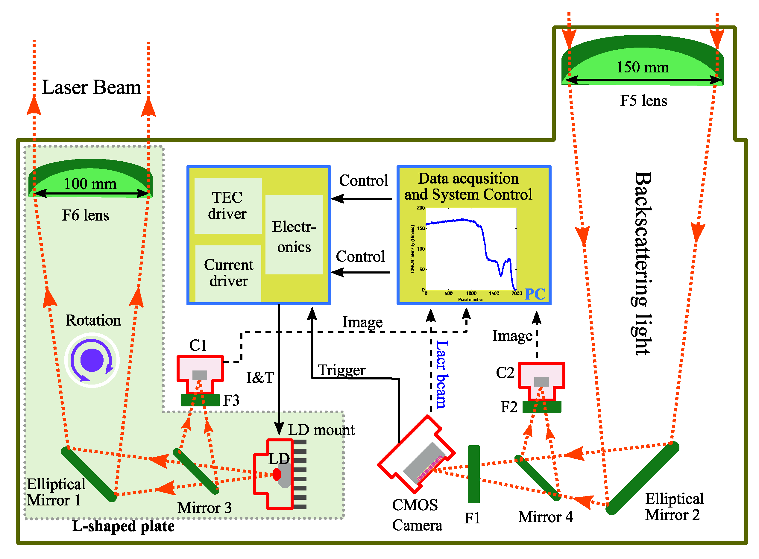
2. Instrumentation
2.1. Optomechanics and Electronics
2.2. Signal Acquisition and Processing
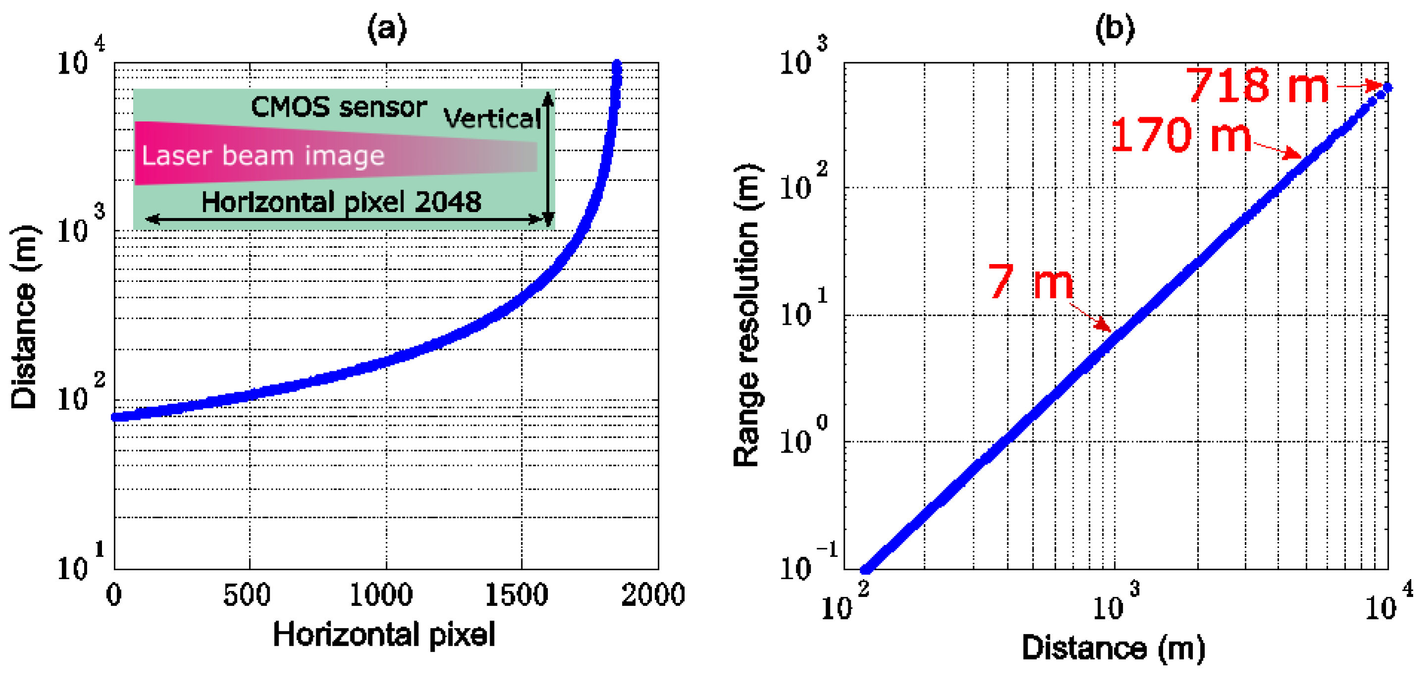
2.3. Pixel-Distance Relationship
3. Measurements
3.1. System Performance Validation
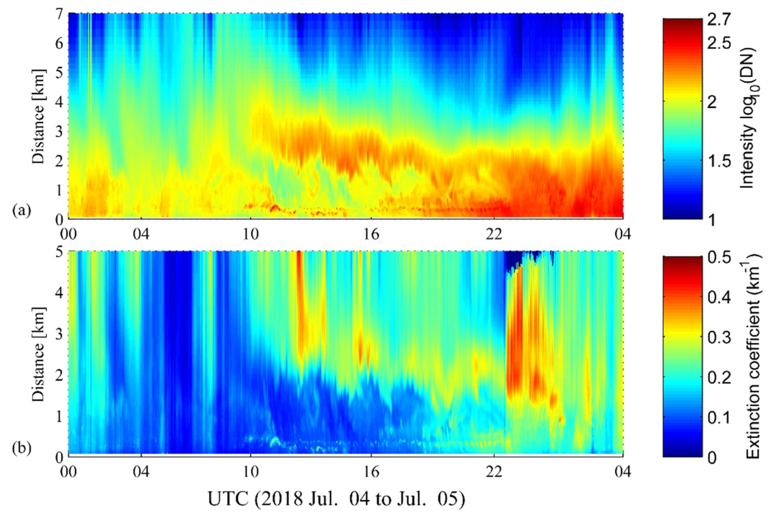
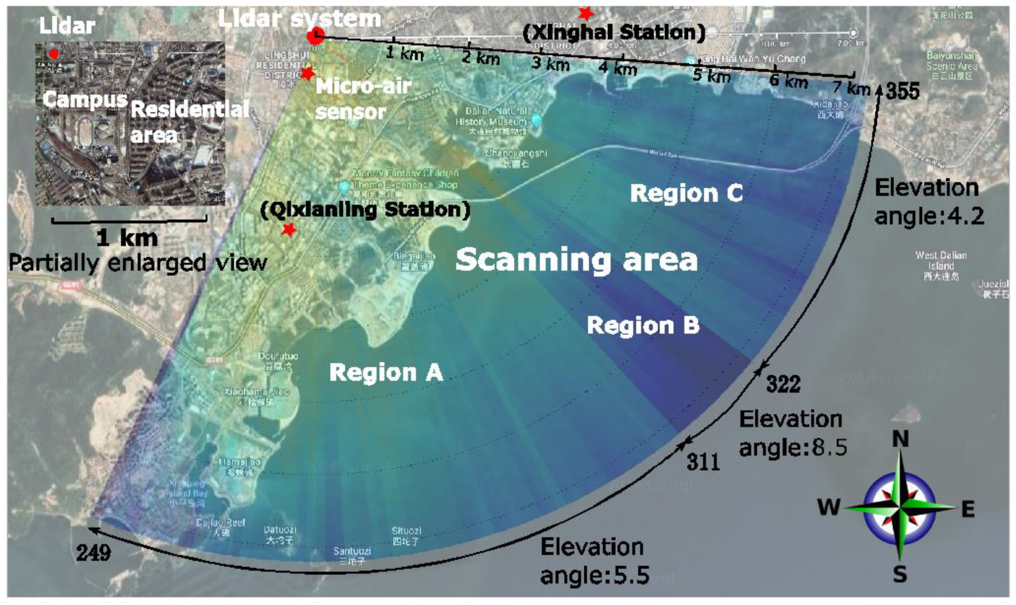
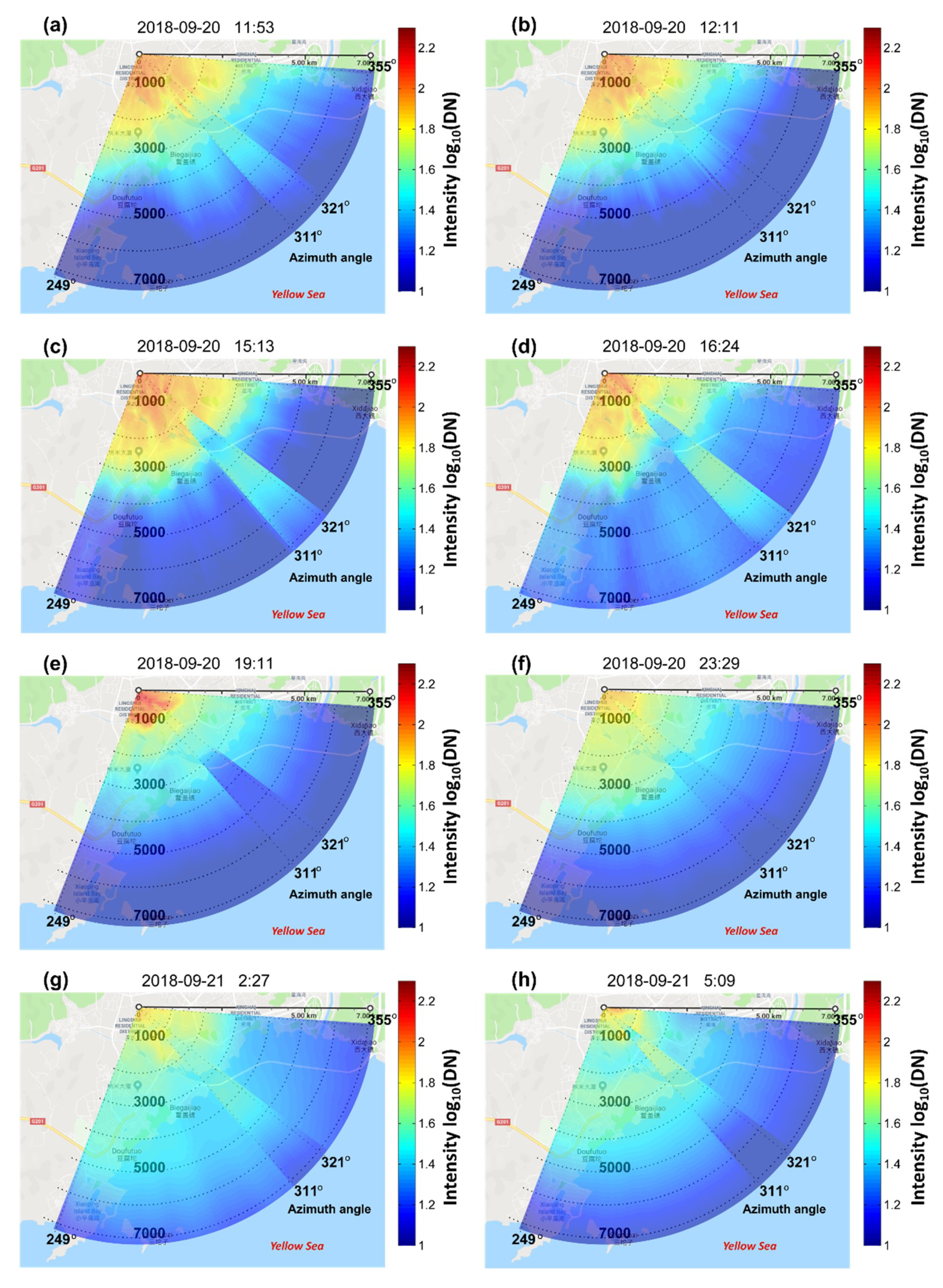
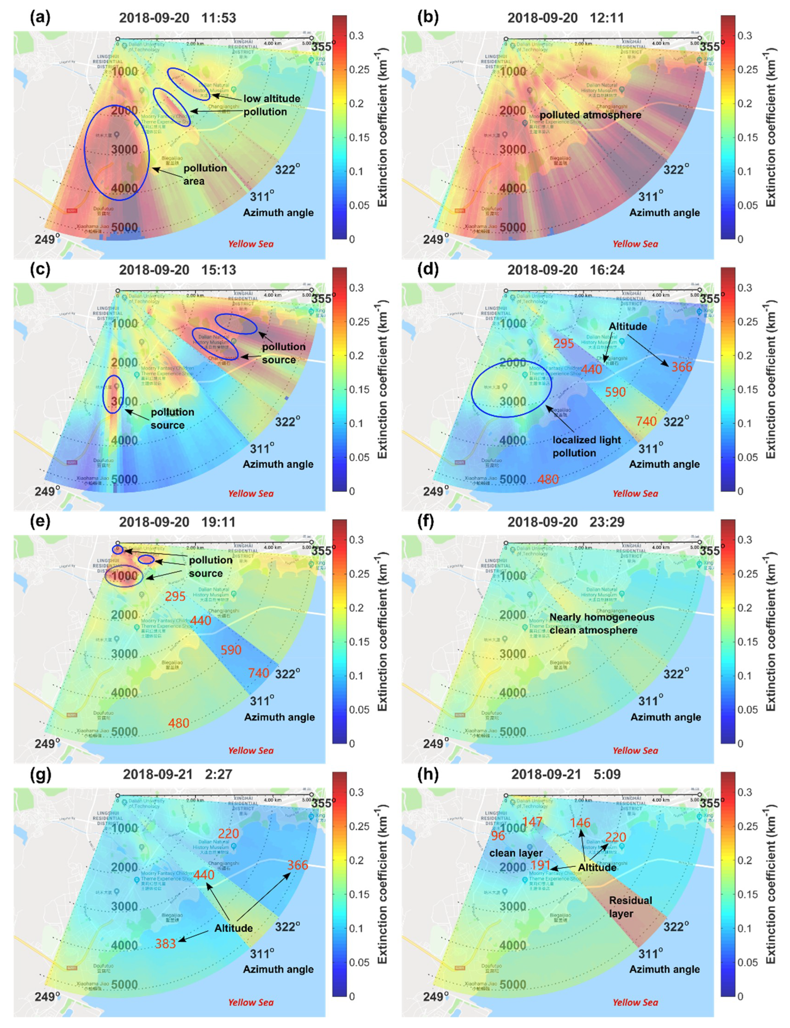
3.2. Atmospheric Horizontal Scanning Measurements for Pollution Source Tracking
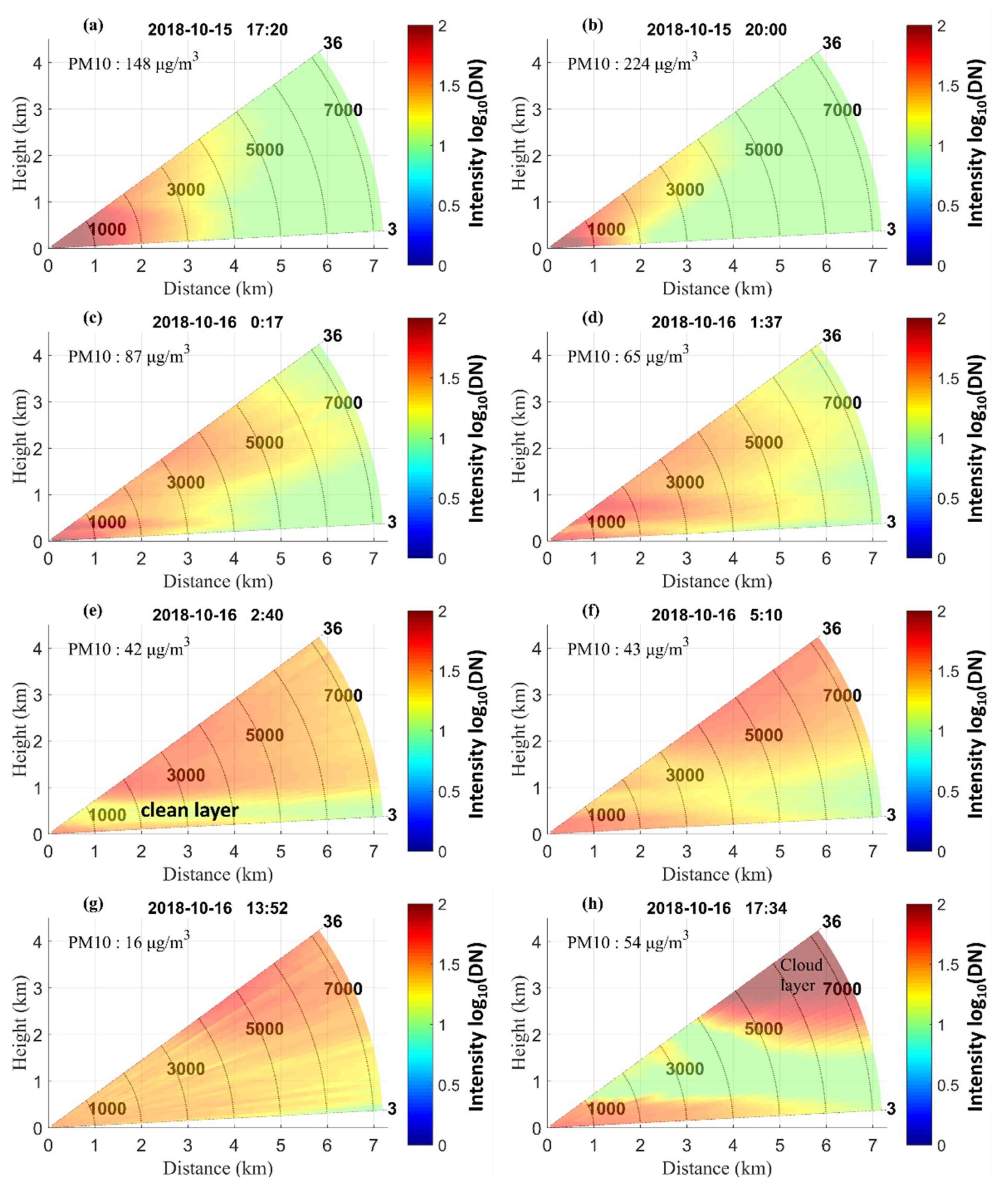
3.3. Atmospheric Vertical Scanning Measurements
4. Discussion
5. Conclusions
6. Patents
Supplementary Materials
Author Contributions
Funding
Acknowledgments
Conflicts of Interest
References
- Engelmann, R.; Kanitz, T.; Baars, H.; Heese, B.; Althausen, D.; Skupin, A.; Wandinger, U.; Komppula, M.; Stachlewska, I.S.; Amiridis, V.; et al. The automated multiwavelength Raman polarization and water-vapor lidar Polly(XT): The neXT generation. Atmos. Meas. Tech. 2016, 9, 1767–1784. [Google Scholar] [CrossRef]
- Radlach, M.; Behrendt, A.; Wulfmeyer, V. Scanning rotational Raman lidar at 355 nm for the measurement of tropospheric temperature fields. Atmos. Chem. Phys. 2008, 8, 159–169. [Google Scholar] [CrossRef]
- Mamouri, R.E.; Papayannis, A.; Amiridis, V.; Muller, D.; Kokkalis, P.; Rapsomanikis, S.; Karageorgos, E.T.; Tsaknakis, G.; Nenes, A.; Kazadzis, S.; et al. Multi-wavelength Raman lidar, sun photometric and aircraft measurements in combination with inversion models for the estimation of the aerosol optical and physico-chemical properties over Athens, Greece. Atmos. Meas. Tech. 2012, 5, 1793–1808. [Google Scholar] [CrossRef]
- Wu, S.H.; Song, X.Q.; Liu, B.Y.; Dai, G.Y.; Liu, J.T.; Zhang, K.L.; Qin, S.G.; Hua, D.X.; Gao, F.; Liu, L.P. Mobile multi-wavelength polarization Raman lidar for water vapor, cloud and aerosol measurement. Opt. Express 2015, 23, 33870–33892. [Google Scholar] [CrossRef]
- Rogers, R.R.; Hair, J.W.; Hostetler, C.A.; Ferrare, R.A.; Obland, M.D.; Cook, A.L.; Harper, D.B.; Burton, S.P.; Shinozuka, Y.; McNaughton, C.S.; et al. NASA LaRC airborne high spectral resolution lidar aerosol measurements during MILAGRO: Observations and validation. Atmos. Chem. Phys. 2009, 9, 4811–4826. [Google Scholar] [CrossRef]
- Muller, D.; Hostetler, C.A.; Ferrare, R.A.; Burton, S.P.; Chemyakin, E.; Kolgotin, A.; Hair, J.W.; Cook, A.L.; Harper, D.B.; Rogers, R.R.; et al. Airborne Multiwavelength High Spectral Resolution Lidar (HSRL-2) observations during TCAP 2012: Vertical profiles of optical and microphysical properties of a smoke/urban haze plume over the northeastern coast of the US. Atmos. Meas. Tech. 2014, 7, 3487–3496. [Google Scholar] [CrossRef]
- Sun, W.B.; Hu, Y.X.; MacDonnell, D.G.; Weimer, C.; Baize, R.R. Technique to separate lidar signal and sunlight. Opt. Express 2016, 24, 12949–12954. [Google Scholar] [CrossRef]
- Marchant, C.C.; Wilkerson, T.D.; Bingham, G.E.; Zavyalov, V.V.; Andersen, J.M.; Wright, C.B.; Cornelsen, S.S.; Martin, R.S.; Silva, P.J.; Hatfield, J.L. Aglite lidar: A portable elastic lidar system for investigating aerosol and wind motions at or around agricultural production facilities. J. Appl. Remote Sens. 2009, 3, 033511. [Google Scholar] [CrossRef]
- Behrendt, A.; Pal, S.; Wulfmeyer, V.; Valdebenito, A.M.; Lammel, G. A novel approach for the characterization of transport and optical properties of aerosol particles near sources—Part I: Measurement of particle backscatter coefficient maps with a scanning UV lidar. Atmos. Environ. 2011, 45, 2795–2802. [Google Scholar] [CrossRef]
- Stachlewska, I.S.; Neuber, R.; Lampert, A.; Ritter, C.; Wehrle, G. AMALi—The Airborne Mobile Aerosol Lidar for Arctic research. Atmos. Chem. Phys. 2010, 10, 2947–2963. [Google Scholar] [CrossRef]
- Dubey, P.K.; Jain, S.L.; Arya, B.C.; Ahammed, Y.N.; Kumar, A.; Shukla, D.K.; Kulkarni, P.S. Indigenous design and development of a micro-pulse lidar for atmospheric studies. Int. J. Remote Sens. 2011, 32, 337–351. [Google Scholar] [CrossRef]
- Sicard, M.; Izquierdo, R.; Alarcon, M.; Belmonte, J.; Comeron, A.; Baldasano, J.M. Near-surface and columnar measurements with a micro pulse lidar of atmospheric pollen in Barcelona, Spain. Atmos. Chem. Phys. 2016, 16, 6805–6821. [Google Scholar] [CrossRef]
- Parracino, S.; Richetta, M.; Gelfusa, M.; Malizia, A.; Bellecci, C.; de Leo, L.; Perrimezzi, C.; Fin, A.; Forin, M.; Giappicucci, F.; et al. Real-time vehicle emissions monitoring using a compact LiDAR system and conventional instruments: First results of an experimental campaign in a suburban area in southern Italy. Opt. Eng. 2016, 55, 103107. [Google Scholar] [CrossRef]
- Xie, H.L.; Zhou, T.; Fu, Q.; Huang, J.P.; Huang, Z.W.; Bi, J.R.; Shi, J.S.; Zhang, B.D.; Ge, J.M. Automated detection of cloud and aerosol features with SACOL micro-pulse lidar in northwest China. Opt. Express 2017, 25, 30732–30753. [Google Scholar] [CrossRef] [PubMed]
- Pappalardo, G.; Amodeo, A.; Apituley, A.; Comeron, A.; Freudenthaler, V.; Linne, H.; Ansmann, A.; Bosenberg, J.; D′Amico, G.; Mattis, I.; et al. EARLINET: Towards an advanced sustainable European aerosol lidar network. Atmos. Meas. Tech. 2014, 7, 2389–2409. [Google Scholar] [CrossRef]
- Lewis, J.R.; Campbell, J.R.; Welton, E.J.; Stewart, S.A.; Haftings, P.C. Overview of MPLNET, Version 3, Cloud Detection. J. Atmos. Ocean Tech. 2016, 33, 2113–2134. [Google Scholar] [CrossRef]
- Nishizawa, T.; Sugimoto, N.; Matsui, I.; Shimizu, A.; Higurashi, A.; Jin, Y. The Asian dust and aerosol lidar observation network (Ad-Net): Strategy and progress. Epj Web Conf. 2016, 119, 19001. [Google Scholar] [CrossRef]
- Baars, H.; Kanitz, T.; Engelmann, R.; Althausen, D.; Heese, B.; Komppula, M.; Preissler, J.; Tesche, M.; Ansmann, A.; Wandinger, U.; et al. An overview of the first decade of Polly(NET): An emerging network of automated Raman-polarization lidars for continuous aerosol profiling. Atmos. Chem. Phys. 2016, 16, 5111–5137. [Google Scholar] [CrossRef]
- Wandinger, U.; Freudenthaler, V.; Baars, H.; Amodeo, A.; Engelmann, R.; Mattis, I.; Gross, S.; Pappalardo, G.; Giunta, A.; D′Amico, G.; et al. EARLINET instrument intercomparison campaigns: Overview on strategy and results. Atmos. Meas. Tech. 2016, 9, 1001–1023. [Google Scholar] [CrossRef]
- Caicedo, V.; Rappengluck, B.; Lefer, B.; Morris, G.; Toledo, D.; Delgado, R. Comparison of aerosol lidar retrieval methods for boundary layer height detection using ceilometer aerosol backscatter data. Atmos. Meas. Tech. 2017, 10, 1609–1622. [Google Scholar] [CrossRef]
- Peng, J.; Grimmond, C.S.B.; Fu, X.S.; Chang, Y.Y.; Zhang, G.L.; Guo, J.B.; Tang, C.Y.; Gao, J.; Xu, X.D.; Tan, J.G. Ceilometer-based analysis of Shanghai′s boundary layer height under rain- and fog-free conditions. J. Atmos. Ocean Tech. 2017, 34, 749–764. [Google Scholar] [CrossRef]
- Adam, M.; Turp, M.; Horseman, A.; Ordonez, C.; Buxmann, J.; Sugier, J. From operational ceilometer network to operational lidar network. Epj Web Conf. 2016, 119, 27007. [Google Scholar] [CrossRef]
- Spuler, S.M.; Mayor, S.D. Scanning eye-safe elastic backscatter lidar at 1.54 μm. J. Atmos. Ocean Tech. 2004, 22, 696. [Google Scholar] [CrossRef]
- He, T.Y.; Stanic, S.; Gao, F.; Bergant, K.; Veberic, D.; Song, X.Q.; Dolzan, A. Tracking of urban aerosols using combined LIDAR-based remote sensing and ground-based measurements. Atmos. Meas. Tech. 2012, 5, 891–900. [Google Scholar] [CrossRef]
- Strawbridge, K.B. Developing a portable, autonomous aerosol backscatter lidar for network or remote operations. Atmos. Meas. Tech. 2013, 6, 801–816. [Google Scholar] [CrossRef]
- Xie, C.B.; Zhao, M.; Wang, B.X.; Zhong, Z.Q.; Wang, L.; Liu, D.; Wang, Y.J. Study of the scanning lidar on the atmospheric detection. J. Quant. Spectrosc. Rad. Transf. 2015, 150, 114–120. [Google Scholar] [CrossRef]
- Chiang, C.W.; Das, S.K.; Chiang, H.W.; Nee, J.B.; Sun, S.H.; Chen, S.W.; Lin, P.H.; Chu, J.C.; Su, C.S.; Su, L.S. A new mobile and portable scanning lidar for profiling the lower troposphere. Geosci. Instrum. Meth. 2015, 4, 35–44. [Google Scholar] [CrossRef]
- Weekley, R.A.; Goodrich, R.K.; Cornman, L.B. Aerosol plume detection algorithm based on image segmentation of scanning atmospheric lidar data. J. Atmos. Ocean Tech. 2016, 33, 697–712. [Google Scholar] [CrossRef]
- De Wekker, S.F.J.; Mayor, S.D. Observations of Atmospheric Structure and Dynamics in the Owens Valley of California with a Ground-Based, Eye-Safe, Scanning Aerosol Lidar. J. Appl. Meteorol. Clim. 2009, 48, 1483–1499. [Google Scholar] [CrossRef]
- Mei, L.; Brydegaard, M. Atmospheric aerosol monitoring by an elastic Scheimpflug lidar system. Opt. Express 2015, 23, 247841. [Google Scholar] [CrossRef]
- Mei, L.; Guan, P.; Yang, Y.; Kong, Z. Atmospheric extinction coefficient retrieval and validation for the single-band Mie-scattering Scheimpflug lidar technique. Opt. Express 2017, 25, A628–A638. [Google Scholar] [CrossRef]
- Mei, L.; Guan, P. Development of an atmospheric polarization Scheimpflug lidar system based on a time-division multiplexing scheme. Opt. Lett. 2017, 42, 3562–3565. [Google Scholar] [CrossRef]
- Sun, G.D.; Qin, L.A.; Hou, Z.H.; Jing, X.; He, F.; Tan, F.F.; Zhang, S.L. Small-scale Scheimpflug lidar for aerosol extinction coefficient and vertical atmospheric transmittance detection. Opt. Express 2018, 26, 7423–7436. [Google Scholar] [CrossRef]
- Brydegaard, M.; Gebru, A.; Svanberg, S. Super resolution laser radar with blinking atmospheric particles—Application to interacting flying insects. PIER 2014, 147, 141–151. [Google Scholar] [CrossRef]
- Malmqvist, E.; Brydegaard, M.; Alden, M.; Bood, J. Scheimpflug Lidar for combustion diagnostics. Opt. Express 2018, 26, 14842–14858. [Google Scholar] [CrossRef]
- Brydegaard, M.; Malmqvist, E.; Jansson, S.; Larsson, J.; Torok, S.; Zhao, G.Y. The Scheimpflug lidar method. Proc. Spie 2017, 10406, 104060I. [Google Scholar]
- Brydegaard, M.; Larsson, J.; Török, S.; Malmqvist, E.; Zhao, G.; Jansson, S.; Andersson, M.; Svanberg, S.; Åkesson, S.; Laurell, F.; et al. Short-wave infrared atmospheric Scheimpflug lidar. In Proceedings of the EPJ Web of Conferences, Bucharest, Romania, 25–30 June 2017. [Google Scholar]
- Mei, L.; Kong, Z.; Liu, Z.; Zhang, L.; Guan, P. Atmospheric pollution monitoring by employing a 450-nm Scheimpflug lidar system. Sensors 2018, 18, 1880. [Google Scholar]
- Mei, L.; Kong, Z.; Ma, T. Dual-wavelength Mie-scattering Scheimpflug lidar system developed for the studies of the aerosol extinction coefficient and the Angstrom exponent. Opt. Express 2018, 26, 31942–31956. [Google Scholar] [CrossRef]
- Mei, L.; Guan, P.; Kong, Z. Remote sensing of atmospheric NO2 by employing the continuous-wave differential absorption lidar technique. Opt. Express 2017, 25, A953–A962. [Google Scholar] [CrossRef]
- Mei, L.; Zhang, L.; Kong, Z.; Li, H. Noise modeling, evaluation and reduction for the atmospheric lidar technique employing an image sensor. Opt. Commun. 2018, 426, 463–470. [Google Scholar] [CrossRef]
- Klett, J.D. Lidar inversion with variable backscatter extinction ratios. Appl. Opt. 1985, 24, 1638–1643. [Google Scholar] [CrossRef]
- Kovalev, V.A.; Eichinger, W.E. Elastic Lidar: Theory, Practice, and Analysis Methods; John Wiley & Sons: Hoboken, NJ, USA, 2004. [Google Scholar]


© 2019 by the authors. Licensee MDPI, Basel, Switzerland. This article is an open access article distributed under the terms and conditions of the Creative Commons Attribution (CC BY) license (http://creativecommons.org/licenses/by/4.0/).
Share and Cite
Liu, Z.; Li, L.; Li, H.; Mei, L. Preliminary Studies on Atmospheric Monitoring by Employing a Portable Unmanned Mie-Scattering Scheimpflug Lidar System. Remote Sens. 2019, 11, 837. https://doi.org/10.3390/rs11070837
Liu Z, Li L, Li H, Mei L. Preliminary Studies on Atmospheric Monitoring by Employing a Portable Unmanned Mie-Scattering Scheimpflug Lidar System. Remote Sensing. 2019; 11(7):837. https://doi.org/10.3390/rs11070837
Chicago/Turabian StyleLiu, Zhi, Limei Li, Hui Li, and Liang Mei. 2019. "Preliminary Studies on Atmospheric Monitoring by Employing a Portable Unmanned Mie-Scattering Scheimpflug Lidar System" Remote Sensing 11, no. 7: 837. https://doi.org/10.3390/rs11070837
APA StyleLiu, Z., Li, L., Li, H., & Mei, L. (2019). Preliminary Studies on Atmospheric Monitoring by Employing a Portable Unmanned Mie-Scattering Scheimpflug Lidar System. Remote Sensing, 11(7), 837. https://doi.org/10.3390/rs11070837