An Efficient Framework for Mobile Lidar Trajectory Reconstruction and Mo-norvana Segmentation

Abstract

Mobile laser scanning (MLS, or mobile lidar) is a 3-D data acquisition technique that has been widely used in a variety of applications in recent years due to its high accuracy and efficiency. However, given the large data volume and complexity of the point clouds, processing MLS data can be still challenging with respect to effectiveness, efficiency, and versatility. This paper proposes an efficient MLS data processing framework for general purposes consisting of three main steps: trajectory reconstruction, scan pattern grid generation, and Mo-norvana (Mobile Normal Variation Analysis) segmentation. We present a novel approach to reconstructing the scanner trajectory, which can then be used to structure the point cloud data into a scan pattern grid. By exploiting the scan pattern grid, point cloud segmentation can be performed using Mo-norvana, which is developed based on our previous work for processing Terrestrial Laser Scanning (TLS) data, normal variation analysis (Norvana). In this work, with an unorganized MLS point cloud as input, the proposed framework can complete various tasks that may be desired in many applications including trajectory reconstruction, data structuring, data visualization, edge detection, feature extraction, normal estimation, and segmentation. The performance of the proposed procedures are experimentally evaluated both qualitatively and quantitatively using multiple MLS datasets via the results of trajectory reconstruction, visualization, and segmentation. The efficiency of the proposed method is demonstrated to be able to handle a large dataset stably with a fast computation speed (about 1 million pts/sec. with 8 threads) by taking advantage of parallel programming.

1. Introduction

Mobile Laser Scanning (MLS, or mobile lidar) is an accurate and efficient approach to acquire detailed, 3-D data, based on Light Detection And Ranging (lidar) technology from a mobile platform, typically a vehicle. In addition to the laser scanner, one or multiple Global Positioning System (GPS)/ Global Navigation Satellite System (GNSS) receivers and an Inertial Measurement Unit (IMU) are also integrated on a mobile lidar system, to measure the position and state (orientation) of the moving platform, such that the point cloud can be directly georeferenced. MLS is advantageous over Terrestrial Laser Scanning (TLS) in terms of mapping efficiency for long sections of roadway. While local accuracy is generally better with TLS, network accuracy can be similar between the two systems. MLS is advantageous over Airborne Laser Scanning (ALS), because it is significantly more accurate, and can be deployed with much fewer logistics. In recent years, MLS has been widely used in a variety of applications, such as engineering surveying, asset management, construction, deformation monitoring, and so forth (Olsen, et al. [1]), where in some cases (e.g., culture heritage), MLS can also serve as complementary data combined with other data, such as TLS and ALS (Balsa-Barreiro and Fritsch [2]).

In addition to the point cloud data acquired by the scanner, the system also provides an accurate trajectory of the platform as it travels. The trajectory is normally referenced to the IMU but is computed-based on a combination of the GPS/GNSS receiver(s), IMU, and Distance Measuring Instruments (DMI) to improve its resolution, accuracy, and robustness (Che, et al. [3]).

Despite the many advantages of MLS technology, there are numerous challenges and open research questions related to processing mobile lidar data. A variety of approaches have been developed to help extract meaningful information from mobile lidar data, as well as to simplify the processing, which can be challenging, given the large size and complexity of mobile lidar datasets. Some methods require the trajectory as the starting point, since it serves as a key assumption to determine the location of the road surface. Algorithms utilizing the trajectory to aid in processing will be further discussed in detail in Section 2.1. Additional approaches have been developed to segment mobile lidar data into distinct objects for subsequent analysis, which will be summarized in Section 2.2. Regardless, despite the success in applying these approaches to a test dataset for the specific application, there are three principal limitations or challenges for these approaches:

A high-accuracy trajectory used for generating the point cloud is not always provided with mobile lidar point clouds, since it is usually considered as secondary data that may not be directly useful to the end users. In some cases, the trajectory may only be provided as a simplified reference to the end users. Other times, it may not be provided in the same coordinate system as the end point cloud, since the initial processing is often completed in 3-D, earth centered, earth fixed (ECEF) coordinates, compared with the mapping projection desired for the point cloud and other end products. Moreover and most importantly, in most systems, the trajectory exported from the processing software is the position and state of the IMU, rather than that of the scanner itself. Transforming the IMU trajectory to the scanner trajectory requires additional configuration and calibration information, which would rarely be available to the end users of the data. Further, many end users would lack the appropriate geomatics knowledge necessary to apply the calibration parameters correctly. Use of the IMU trajectory instead of the scanner trajectory may be adequate for some applications; however, it can lead to significant errors in others. Although several approaches exist to estimate the scanner trajectory, the approaches can only cope with specific scenarios such as a well-defined, urban street corridor or a tunnel (e.g., Rodríguez-Cuenca, et al. [4], Puente, et al. [5]). In many cases, these estimations are very coarse, and are meant to support a specific application.

Some segmentation and classification methods are limited to scenes with specific objects present. Certain approaches use a hierarchical structure to segment and classify the entire scene. In such processes, segmenting one class of objects can be dependent on the extraction and recognition result of another class. As an example, some methods define the road surface using the curbs to serve as a boundary for extraction (see Section 2.2). However, curbs may not exist along portions of the road, particularly in rural settings, causing the algorithm to fail. Failure to extract the road surface then leads to cascading failures in extracting and segmenting other objects that rely on properly identifying the road surface. Additionally, to recognize each class, a set of parameters based on the scene, object, and the hierarchical structure are required; hence, such methods can be sensitive to the parameter selection, especially for a scene containing a variety of objects to classify.

Most approaches require substantial processing time to implement, limiting their practical application to datasets larger than a few million points, which are not representative of most mobile lidar datasets (tens to hundreds of millions of points). In particular, for approaches based on a supervised learning process, a complex feature extraction at each point can be computationally expensive. Moreover, manually generating the training dataset sufficient for segmentation and classification of the mobile lidar data can also be time consuming in practice. Some methods down-sample the data, or resample the data into voxels to reduce the computation time, but these approaches require the user to balance the processing strategy between the loss of detail and an increase in computation time. Furthermore, because the point density of mobile lidar data are highly variable, substantial data gaps occur when a small voxel size is desired.

To overcome these three challenges, we propose a novel, generalized, efficient mobile lidar data processing framework, which solely inputs an unorganized point cloud to perform trajectory reconstruction, visualization, feature extraction, normal estimation, and segmentation. The products of this framework are suitable for utilization in different analyses to support a wide range of applications. This framework consists of three main steps: (1) Reconstructing the scanner trajectory; (2) structuring the point cloud data into an organized grid corresponding to the scan acquisition pattern; and (3) performing edge detection, normal estimation, and segmentation based on mobile lidar normal variation analysis (Mo-norvana).

2. Related Work

2.1. Use of Mobile Lidar Trajectory Information

The trajectory data is often considered as a secondary dataset, and may not necessarily be provided with the mobile lidar point cloud. Nevertheless, many advanced processing methods for mobile lidar data take advantage of the trajectory information. Based on the information provided by the trajectory data, there are three main goals that can be achieved when processing mobile lidar data: Data partitioning, ground extraction, and radiometric calibration (

Table 1. Summary of the mobile lidar processing methods using trajectory data.

Applications	Use of Trajectory Data			References
	Data Partitioning	Road Extraction	Radiometric Calibration
Road surface extraction	✓	✓		Chen, et al. [6]
		✓		Wang, et al. [7]
	✓	✓		Holgado-Barco, et al. [8]
	✓			Wang, et al. [9]
	✓			Wu, et al. [10]
	✓	✓		Zai, et al. [11]
Road marking extraction	✓	✓		Guan, et al. [12]
			✓	Kumar, et al. [13]
			✓	Yu, et al. [14]
	✓	✓		Yan, et al. [15]
	✓	✓	✓	Soilán, et al. [16]
	✓	✓		Jung, et al. [17]
Pole-like object extraction	✓			Yu, et al. [18]
	✓	✓		Teo and Chiu [19]
	✓			Wang, et al. [20]
Asset condition assessment			✓	Teo and Yu [21]
			✓	Ai and Tsai [22]
General segmentation and classification	✓			Pu, et al. [23]
	✓			González-Jorge, et al. [24]
		✓		Li, et al. [25]

). It is important to note that in many of these studies, the IMU trajectory, rather than the scanner trajectory, is likely utilized, which can lead to additional errors in the subsequent geometric computations, since the IMU and scanner cannot be physically co-located.

(1) Data partitioning

Mobile lidar data is usually collected along a road, and the point cloud data can contain tens to hundreds of millions of points in a single pass through the area of interest. Consequently, the point cloud data often need to be preprocessed in order to reduce the computation complexity, as well as the overall processing time. A common approach is to down-sample the mobile lidar data directly based upon the trajectory. For example, González-Jorge, et al. [24] and Varela-González, et al. [26] resample the trajectory points using a pre-defined speed, and then subsequently reduce the point cloud to only those points corresponding to the resampled trajectory points based on their time stamps. As another example, Guan, et al. [12] and Yu, et al. [14] extract profiles orthogonal to the trajectory, with a given profile width and sampling interval for performing analyses on each profile. Although the results of these methods are often effective in using the data from a practical perspective, the fact remains that there can still be a significant loss of information from the ignored data. Without removing the points during the partition procedure, other methods divide the data into sections or tiles, such that each section can be processed separately to reduce the computation complexity (e.g., Chen, et al. [6], Holgado-Barco, et al. [8], Wu, et al. [10], Soilán, et al. [16], Jung, et al. [17], Teo and Chiu [19], Pu, et al. [23]). Furthermore, depending on the desired analysis, the refinement of the data partition can be achieved by merging multiple profiles to generate a series of overlapping tiles (e.g., Zai, et al. [11], Wang, et al. [20]), or by dividing a profile based on some other constraints, such as the slope of the roadway (e.g., Wang, et al. [9]).

(2) Road extraction

In addition to providing the path of the data collection, the trajectory data is also helpful for extracting the road surface. With the assumption that the trajectory is acquired at a consistent height above the road surface on which the mobile lidar system travels, it becomes straightforward to select a seed point on the road surface. Then, by defining the boundaries of the road (e.g., curb) and/or the characteristics of the road surface (e.g., elevation, slope, etc.), the road surface can be extracted starting from the seed point(s). For instance, Chen, et al. [6] first filter out the points that are distant from the trajectory, then estimate the ground elevation based upon the distributions of elevations of the mobile lidar points (using the assumption that the majority of mobile lidar points will be on the road surface). They also consider the scan angle in bounding that estimate. Similarly, Teo and Chiu [19] first estimate the elevation of the road, using the height of the trajectory, and then based on the normal vector and horizontal range to the road centerlines generated from the trajectory, the road surface is segmented. Holgado-Barco, et al. [8] also extract the ground points by considering scan angles within a given range threshold. Wang, et al. [7] detect the road boundaries by using elevation variance in the orthogonal direction to the trajectory as a constraint for each point while the elevation is used to filter other objects. Similar with this method, Guan, et al. [12] and Ibrahim and Lichti [27] extract the curb as the road boundary to help determine the road surface based on point density and elevation variance, respectively. Zai, et al. [11] propose a method for road boundary extraction using a graph cut approach based on energy minimization. Additionally, some other methods use slope or point density to determine the road surface directly such as Li, et al. [25] and Varela-González, et al. [26].

(3) Radiometric calibration

Some applications of mobile lidar data analysis can exploit the radiometric information provided as intensity values (return signal strength) in lidar point clouds. When utilizing this information, a radiometric calibration is usually desired, because the intensity is impacted by various factors, such as range, angle of incidence, materials, environmental conditions, and so on (Kashani, et al. [28]). Because computing the range and angle of incidence for a point requires knowledge of the position of the scanner when acquiring each point, the trajectory data can be essential for calculating the appropriate corrections to normalize the intensity values, or to use them to estimate the reflectance. For example, Teo and Yu [21] developed an approach to normalize intensity values across the road surface.

Others have taken advantage of the corrected intensity values to extract road markings (e.g., Kumar, et al. [13], Yu, et al. [14], Soilán, et al. [16]). Lastly, Ai and Tsai [22] perform a radiometric calibration to convert the intensity values to a measure of retro-reflectivity suitable for evaluating the condition of traffic signs.

2.2. Segmentation for Mobile Lidar Data

Point cloud segmentation groups points based upon their similarity of position, normals, color, intensity and/or other attributes. By conducting processing and analysis to the segments rather than individual points, the segmentation results can support various applications effectively and efficiently. A significant number of approaches have been proposed for extracting or classifying specific objects such as pole-like objects (e.g., traffic signs, street lamps, and power poles), road surface, road boundary (e.g., curbs), trees, and so forth, to support transportation applications, such as developing inventories for asset management and condition monitoring. Because these approaches have been summarized in prior work (e.g., Williams, et al. [29], Ma, et al. [30], Che, et al. [3]), herein, we mainly focus on reviewing those generic approaches able to segment the complete scene for clarity of presentation.

Several methods have been demonstrated to effectively segment TLS data, which are collected with a similar view of an object as a mobile lidar. Nevertheless, it can still be challenging to apply the methods developed for TLS data to segment mobile lidar data, due to differences in the point density and geometric arrangement of the points between the two systems (Che, et al. [3]). Typically, a TLS acquires data from a stationary platform with a constant angular increment both horizontally and vertically. Thus, in a single scan, the point density will decrease with increasing range and angles of incidence, yet requiring multiple scans can help achieve the desired spatial resolution and minimize data gaps. In contrast, although the scanner on a mobile lidar system acquires each scanline similar to the TLS, the spatial resolution on the other direction (scanline spacing) is a function of the driving speed, which, although it is relatively consistent, it is typically much larger than the spacing between points within a scanline. Hence, some techniques for neighbor searching such as k-Nearest Neighbor (k-NN) or spherical neighbors, which are commonly used in algorithms for processing TLS data, may provide an imbalanced distribution of neighbor points, especially at close ranges where most searched neighbors can concentrate along the same scanline as the given point (Figure 1). Consequently, this imbalance of neighbor point distribution can affect the following computations and analyses, based upon the flawed assumption that the points are more or less evenly distributed.

To overcome the challenge of imbalanced data density in point cloud segmentation for mobile lidar data, some methods resample or organize the data through voxelization. For example, Vo, et al. [31] first organize the point cloud into voxels, such that an octree structure can be simply exploited for neighbor searching. Then, feature estimation describes each voxel to evaluate the similarity between two adjacent voxels in the following region growing step. Finally, to further merge unlabeled points to the existing segments, a refinement is conducted by distinguishing boundary voxels from the planar voxels to cope with both planar and non-planar segments. Some works discuss optimal definition of neighbors for feature extraction, segmentation, and classification (e.g., Demantke, et al. [32], Weinmann, et al. [33], Hackel, et al. [34]). For instance, utilizing the neighbor selection approach proposed by Demantke, et al. [32], Yang and Dong [35] first label the points as linear, planar, or spherical points based on a Principal Component Analysis (PCA). These labeled points are then merged based on different rules, and a normalized cut approach, based on a similarity measurement, is used to refine the segmentation results.

In certain applications using these mobile lidar data, only one or multiple classes of objects may be of interest; hence, many approaches to detect or classify these objects are proposed. Some methods take advantage of ground or road surface extraction, such that the other objects on the ground can be separated and analyzed for the following classification. For example, Pu, et al. [23] first segment the data into ground and non-ground points and then perform clustering with a surface region growing algorithm. Serna and Marcotegui [36] utilize connected components for clustering the non-ground objects with further refinement through a morphological filter. After extracting the ground, Xu, et al. [37] perform an optimal hierarchical clustering approach to the down-sampled non-ground points to segment a mobile lidar point cloud. Unfortunately, these approaches, which rely on the removal of ground points, may fail when multiple objects are clustered together, because they are too close to each other (Wang, et al. [20]). To solve this problem, Li, et al. [25] propose a method to cluster the non-ground points with criteria based on distance and point density.

3. Methodology

Our proposed framework for segmentation consists of three primary steps: Trajectory reconstruction, scan pattern grid generation, and MObile lidar NORmal VAriation Analsysis (Mo-norvana) segmentation (Figure 2). Following a brief summary to introduce the methodology, details of each step will be discussed in the following sections. In this work, the segmentation operates on a single pass of mobile lidar data collected through the area of interest by a single scanner on the mobile platform. The method requires time stamps recorded in the data file, which are a common component in the American Society for Photogrammetry and Remote Sensing (ASPRS) LAS file format (Samberg [38]). (Time stamps are necessary in mobile lidar to link the observations from the various sensors needed to produce the point cloud). In the stage of trajectory reconstruction, with a given scan resolution, the spin rate of the scanner is first estimated, such that the data can be partitioned into a number of scanlines, which can be also considered as the profiles collected in each 360° rotation of scanning measurement. For each scanline, the scan plane and scan origin are then estimated sequentially. Notice that the proposed framework estimates and utilizes the scanner trajectory rather than IMU trajectory. Once the trajectory is reconstructed, the unorganized point cloud data can be structured into a scan pattern grid, which is effective and efficient for data storage, visualization, and processing. In the stage of Mo-norvana, by adjusting the concept of our previous work (Norvana), for TLS data exploiting a similar data structure (Che and Olsen [39]), to cope with mobile lidar data, three steps including point indexing, edge detection, and region growing are conducted in order to segment the mobile lidar data. Notably, the proposed procedures can readily be implemented to take advantage of parallel programming, because most of the processing is performed on each scanline or point independently.

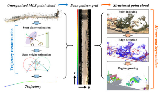
3.1. Trajectory Reconstruction

Typically, the trajectory data records the position and state of the IMU during the data collection based on the combination (e.g., Kalman filtering) of data from the IMU and other sensors, such as the GNSS and DMI. For each scan point, the corresponding origin and orientation of the scanner can be interpolated from the trajectory based on the time stamps associated with the calibration information, such that the scan points can be geo-referenced. Although there are some approaches that utilize the trajectory for mobile lidar data processing and analysis, in a lot of cases, the trajectory data is ignored as an intermediate product, or lost during data transfer and archiving, because they are usually stored in a separate file. Fortunately, many point cloud data formats (e.g., ASPRS LAS) record time stamps for each scan point. In addition, the angular resolution and spin rate of the scanner can be assumed constant during the data collection. Thus, point cloud data with time stamps provide both the geometric and time constraints necessary to enable reverse engineering to reliably reconstruct the trajectory. In this section, we introduce an approach for reconstructing the trajectory with only one parameter required, the scan (angular) resolution dθ, which represents the nominal angular increment (stepping interval) between the scanner observations.

(1) Spin rate estimation

To partition the data into scanlines, the spin rate needs to be estimated first. Based on the assumption of a constant angular resolution (dθ) between pulses, the time between each two adjacent laser beams should be constant. However, in cases where there is no return for a laser beam, nothing is recorded in an unorganized data format for that pulse to indicate that no data were acquired. Thus, we sort all of the points by increasing time, and compute the time difference between each pair of adjacent points. The shortest time difference is then utilized as the initial estimate of the time interval for each observation corresponding to dθ. Because there is some uncertainty in the time differences, we average all of the time differences within a factor of 1.5 of the minimum time interval to obtain the refined time resolution, dt. The spin speed ω and spin rate f of the scanner can be calculated by Equation (1), where the units for dθ, dt, f, and ω are radians, seconds, Hz, and rad/s, respectively.

$$\omega =\frac{2\pi }{f}=\frac{d\theta }{dt}$$

(1)

Using the spin rate, the time stamp of each point can be used to partition the point cloud data into scanlines. Notice that generally both dθ (or number of measurements per rotation) and ω (or f) are reported in the specification of the mobile lidar system. However, the proposed approach solely uses dθ as an input parameter, while ω is derived from dθ because the angle measurement unit is usually more precise and reliable than the spin unit in a scanner.

(2) Scan plane estimation

Although the mobile lidar system continually moves during data acquisition, the time for collecting one scanline, dt, is usually short, and is often synched with the IMU rate, which typically ranges between 100Hz to 2,000 Hz for a mobile lidar system. Hence, the point cloud within each scanline can be assumed to lie approximately within a plane centered at the scanner origin along the trajectory. Since the previous step has partitioned the data into scanlines, we can estimate the scan plane, using sample points in each scanline to compute the orientation (normal vector) of the scan plane, through Principal Component Analysis (PCA), to ensure robustness to errors. Next, we can project each point onto its associated scan plane to obtain its local 2-D coordinates in the coordinate system defined in Figure 3. We first define the scan plane as the x-z plane; hence the normal vector to the scan plane is the y-axis. Nevertheless, defining the arbitrary x-axis and z-axis requires the IMU measurements and corresponding calibration information with the offsets between the scanner and IMU. Fortunately, the roll angle of a vehicle driven on the road is usually small, while the pitch and heading have been calculated through the scan plane estimation. Therefore, by forcing both the y-axis and z-axis to point upward, we can simply define the x-axis as a horizontal vector perpendicular to the y and z axes to form a right-handed coordinate system. Additionally, the scan angle θ of a scan point is defined as the counter-clockwise angle from the z-axis to the laser beam.

(3) Scan origin estimation

With the estimated scan plane and the scan coordinate system defined in the previous step, we can transform the 3-D coordinates of the scan points to local, 2-D coordinates, with the centroid of all points (average coordinates) within each scanline serving as an initial origin. In this section, we present an approach for computing the local coordinates of the scan origin T_p in each scan plane, which can then be utilized as a geo-referenced trajectory point for further computations. Further refinement of T_p is achieved through a least squares adjustment.

Although it is difficult to set constraints using the spatial relationships such as range and scan angle between the scan points and the trajectory point because the scan origin is unknown, the difference in the scan angles Δθ between any two scan points can be easily computed by using the time difference Δt and the spin speed ω, as shown in Equation (2).

$$\Delta \theta =\omega \times \Delta t$$

(2)

We can then utilize geometric relationships between scan points in the line to set up the necessary least squares constraint equations to inversely solve for the scan origin coordinates. The underlying principle is that an inscribed angle is constant on an arc between two known points. Then, based on the locations of any two scan points with a scan angle difference of Δθ in the scanline, the trace of all the possible locations of the scanner origin will lie on an arc (Figure 4). Another arc can be formed with another pair of scan points with the corresponding scan angle difference. The intersection of these two arcs provides an initial estimation of the scan origin. To simplify the estimation of the scan origin in this stage, we only use three scan points such that one point is shared between the two arcs, each formed with one of the other two points. This selection ensures that only one intersection point is available as a scan origin, because the other intersection is the scan point lying on both arcs (e.g., P_j in Figure 4). Note that to improve the spacing between scan points and avoid sharp angles from points spaced too closely, which may lead to large errors in estimating the position of the scan origin, we partition the points from a scanline evenly into three groups based on the total point count in each scanline, and then select the first point from each group for the calculations. Additionally, because the arcs with their corresponding centers can be on either side of the scan points, the proposed approach may initially have two solutions. Thus, we perform a least squares adjustment with one iteration and select the solution with a smaller variance using the constraint model introduced in (3).

Once the initial position of the scan origin is solved using 3 points (2 pairs) in the scanline, we can formulate a constraint for more point pairs considering all points in the scanline, using an equation derived using the cosine law that incorporates the ranges ρ_i and ρ_j of both points, distance between them d_ij, and the difference in scan angles Δθ_ij as shown in Equation (3).

$${\rho }_i^2+{\rho }_j^2-2{\rho }_i{\rho }_j\cos \Delta {\theta }_{ij}=d_{ij}^2$$

(3)

Ironically, although the ranges ρ_i and ρ_j were some of the original raw measurements used to compute the coordinates of the points i and j, this information is generally not stored with the point cloud, and often must be determined inversely. Hence, in Eq. 3, the computed ranges are dependent on the coordinates of the scan origin, which is refined in each iteration of the least squares adjustment.

For the aforementioned reasons of avoiding sharp angles, we select scan point pairs with a constant interval of point counts. Additionally, to ensure the robustness of the computation, we eliminate any point pairs with a scan angle difference larger than 180° from the adjustment. Thus, the number of points (pairs) used for solving the scan origin are a function of the angular distribution and point count in a partition consisting of a scanline. Then, by linearizing the model, a least squares adjustment can be conducted with every pair of points selected as one observation. In each iteration, we compute both the residuals and variance of the observations and remove any observations with a squared residual larger than three times that of the variance for the next iteration. After the least squares adjustment converges or reaches a maximum number of iterations, the coordinates of the scan origin on the scan plane for all the scanlines have been accurately estimated. Because this scan origin is in a local coordinate system, the geo-referenced coordinates of this origin point (which also serves as a trajectory point) can be generated by applying the inverse transformation matrix of the scan.

3.2. Scan Pattern Grid

With the reconstructed trajectory and the defined scan coordinate system, we can structure the mobile lidar data into a scan pattern grid, where each row represents one scanline corresponding to the time stamp of its trajectory point, and each column represents a scan angle (Figure 5). Because each scanline is extracted individually and separated in time, this pattern is not impacted by changes in speed, or any turning of the vehicle.

Because the scan angle and time are independent from the actual geometric distribution of the point cloud, there are several advantages with such a data structure. First of all, structuring the mobile lidar data into a scan pattern grid is versatile for any type of scene, irrespective of topography, the shape of the objects, and other factors.

Second, comparing against other techniques to structure the data into an image or voxels, the proposed grid structure matches with the trajectory and generating the grid does not require any parameter (e.g., cell size) that can result in data gaps or any consolidation of data points. Additionally, even though the proposed data structure is a 2-D grid, it is still able to store all the points without overlapping each other, because every cell represents an individual laser pulse. As a result, it requires minimal space to preserve all of the information from the point cloud data as well as derived attributes. Notice that the no-data cells in the scan pattern grid can be considered as laser pulses with no return, which can provide useful topology information between points (Che and Olsen [40]). Nonetheless, the situation that multiple returns from a laser pulse are recorded is not considered in this work (and is much rarer for MLS) compared with ALS). Furthermore, since the scan pattern grid is a rectangular grid, it can be organized as a set of layers to contain all of the desired attributes at each point to be directly used for efficient data visualization. Finally, advanced computer vision algorithms such as those utilized by Mahmoudabadi, et al. [41] for segmenting TLS data could potentially be applied to the various layers to further process and analyze point cloud data once the challenges such as the large volume of data and any distortion of the objects can be overcome.

3.3. Mo-norvana Segmentation

In our previous work [39], we proposed a fast segmentation method for TLS based on Normal Variation Analysis (Norvana), which exploited the angular grid structure of TLS using the horizontal and vertical scan angles. The basic idea of the Norvana segmentation is to detect edges and smooth surface points by computing the normal variation at each point with its eight neighbors within the angular grid structure, and then group those points enclosed by edges utilizing region growing. In this paper, the concept of angular grid structure is extended to a more generalized concept of the scan pattern grid, which would be applicable to the point cloud collected by a scanner with a pre-defined scan pattern. Unlike the grid structure for TLS where the rows and columns (vertical and horizontal angles) are orthogonal to each other, in a scan pattern grid, because the scanner is often rotated and tilted with respect to the platform, the direction of the trajectory may not be perpendicular to the scan plane. Thus, for some methods exploiting a similar structure generated with existing trajectory data (e.g., Guinard and Vallet [42]), the results can be significantly impacted by the mobile lidar system configuration and scan geometry. As a result, in the proposed Mo-norvana, we adapt the indexing process to the configuration of the mobile lidar system for the neighbor searching, to generate the local 8-neighbor mesh for the normal variation analysis (Figure 6).

(1) Point indexing

By sorting the points based on time stamps and knowing the scanner rotation speed, it is straight forward to search for the adjacent points along the same scanline. To define the adjacent points across the scanline at each point, we first project the points on the adjacent scanlines to the current scanline under analysis using the orientation of its scan plane, and compute the corresponding projected scan angles. Subsequently, we compare the scan angle of the current point under analysis against the projected scan angles, and amongst the points on the adjacent scanlines with a difference less than the angular resolution dθ, the closest points on the adjacent scanlines are selected. Then, the projected distances between a point and its neighbor points in the adjacent scanlines are computed and used for searching for neighbor points on the diagonals. We start searching for the diagonal neighbor points on both sides of each previously searched point on the adjacent scanlines where a point, with the minimum difference between its projected distance and its distance from the starting point. In this way, we can ensure that the neighbor points around each point are approximately evenly distributed.

(2) Silhouette edge detection

A silhouette edge can be defined as the boundary of a shadow caused by an occlusion, and thus represents boundary of the incomplete scanning on an object. We expand the silhouette edge detection based on our original approach to consider errors in the trajectory reconstruction that subsequently propagate to the scan angle computation for detecting the data gaps (i.e., criterion 1 and 2) and keep the original approach for oblique surface and mixed pixels (i.e., criterion 3). In the proposed approach, the silhouette edge points need to meet the following criteria:

Criterion 1: The scan angle difference with any of the point’s adjacent neighbors in along the scanline is larger than two times of angular resolution dθ;

Criterion 2: The distance between the point and its adjacent neighbor meeting the first criterion is larger than a given distance threshold T_{Dist_TIN}, which is the same as the threshold used for generating mesh in the following process;

Criterion 3: The proxy incidence angle computed at a point with each of its adjacent neighbors is less than a given threshold T_α.

As a result, the silhouette edges are detected based on the topological information provided by the scan pattern using the three aforementioned criteria.

(3) Intersection edge detection

In contrast to the silhouette edges caused by the scan geometry, intersection edges are important features for describing the shape of an object. To detect intersection edges, we generate a triangular mesh around each point that is not detected as a silhouette edge point (Figure 6). The point density in a mobile lidar point cloud can vary dramatically due to several factors such as speed, angular resolution, range, and incidence angle. Thus, when searching for the neighbor points along and across the scanline, a minimum edge length of a triangle T_{Dist_TIN} is given to avoid the sharp triangles in the local mesh. Additionally, T_{Dist_TIN} can be also be considered as a function of the target level of detail for the edge detection and segmentation. Next, the normal gradient at each shared edge is computed using the normals of the adjacent two triangles. If any of these normal gradients in a mesh is larger than the given threshold T_ΔNorm, the center point of the mesh is classified as an intersection edge point, otherwise it is classified as a smooth surface point.

(4) Normal estimation

Mo-norvana also supports robust normal estimation for mobile lidar data, which is required in a variety of processing, analysis, and applications. There are two main challenges in estimating normals: (1) Appropriate neighbor selection due to the point density, which can vary dramatically across the scene and leads to poor and scattered normal estimation at close range (Barnea and Filin [43]); and (2) there is no definition of normals at edges (Che and Olsen [39]).

Fortunately, in the proposed method, the eight neighbor points have been judiciously selected, and can be used for robust normal estimation. Moreover, the edge detection and segmentation in Mo-norvana itself can be achieved without estimating normals; hence, an edge point can be simply eliminated for many analyses, or its normal can be computed from one of the smooth surfaces to which it connects. In this case, we show an example for estimating normals by extending the concept of Mo-norvana. For both intersection edge and smooth surface points, the normals of the triangle formed by two shared edges with the minimum averaging normal gradient in a mesh is used to represent the normal vector at the center point of this mesh. As a result, the normals at both the intersection edge and the smooth surface points can be computed robustly and efficiently during the proposed analysis.

(5) Region growing

Once the silhouette and intersection edges are detected, region growing then groups the smooth surface points enclosed by the edge points. All smooth surface points are visited and labeled with a segment index through the process. During the growing process in the same scanline from a seed point, we use the adjacent neighbor points to further exploit the topology from the scan pattern. For growing across the scanline, the neighbors used in the intersection edge detection are incorporated to ensure it is consistent with the normal variation analysis. Notice that because the proposed framework includes normal estimation, the difference in normals between a seed point and its neighbor point is compared against T_ΔNorm to achieve more robust and accurate grouping results.

4. Experiment

4.1. Test Datasets

To evaluate the proposed framework qualitatively and quantitatively, we utilize a mobile lidar dataset (“Phil”) collected by Leica Pegasus:Two mobile lidar system in a suburb area located at Philomath, Oregon, United States for the experiment. The dataset contains 75,637,495 points with an angular resolution of 0.07°. The duration, length, and speed of the data collection are summarized from the trajectory data (

Table 2. Summary of the Data Collection for the Phil Dataset based on the IMU Trajectory.

Duration (s)	Length (m)	Speed (m/s)
		Max.	Min.	Median	Avg.	Std.
154	1319	14.17	0.15	8.15	8.62	2.76

). Note that the dataset for the evaluation covers a wide range of speeds, as well as multiple driving actions (e.g., accelerations, slowdowns, and turns, Figure 7).

We first evaluate the results of trajectory reconstruction, visualization based on the scan pattern grid, and Mo-norvana segmentation. Next, the impact of the driving speed and scan range is further discussed using datasets collected in different lanes. The efficiency of the proposed framework is then demonstrated with several additional datasets with varying sizes, that were collected in the same area of interest. The proposed framework is also tested on a dataset collected on a highway at a higher speed to prove its versatility and robustness.

4.2. Trajectory Reconstruction

To assess the accuracy of the proposed trajectory reconstruction, we first linearly interpolate the IMU trajectory (30,826 points) to match the time stamps from the reconstructed scanner trajectory, which includes 30,607 points. The reason for the resampling is that we find the actual spin rate of the scanner (198 Hz) is slightly slower than the reported rate (200 Hz) in the specification whereas the IMU trajectory is consistent with the IMU rate (200 Hz). Then, we perform statistical analysis on the quality of the trajectory reconstruction, as well as compare the results with the lever arm measurements in the calibration files provided by the manufacturer (

Table 3. Lever arm offset comparison between the reconstructed scanner trajectory and IMU trajectory.

	Vert. Offset (m)	Horz. Offset (m)	3-D Offset (m)
Max.	0.494	0.630	0.672
Min.	0.228	0.356	0.574
Median	0.352	0.483	0.599
Avg.	0.352	0.485	0.599
Std.	0.018	0.020	0.008
Lever arm (Calibration)	0.358	0.491	0.608

). Notice the standard deviations of the vertical and horizontal offsets are significantly higher than the standard deviation of the 3-D offsets. The primary reason for this difference is that we define the scanner coordinate system with the x-axis to be horizontal; hence, the roll angles of the mobile lidar platform are not considered in the proposed approach. At this stage, we only focus on the 3-D offset which is not affected by the state of the mobile lidar platform. The overall difference in the 3-D offset of the reconstructed trajectory compared with the lever arm is less than 0.01m, which is on par with the calibration accuracy (Olsen, et al. [1]).

Despite the fact that the IMU trajectory data and calibration files are provided in this case, it is difficult to convert the IMU trajectory to the scanner trajectory because it is unclear how the coordinate system and the rotation angles are defined for this particular system. Fortunately, we are still able to perform an accuracy assessment by computing the relative positional change between adjacent trajectory points (

Table 4. Comparison between movements in the reconstructed scanner trajectory versus the IMU trajectory based on 30,606 epochs.

	Vert. Error (m)	Horz. Error (m)	3-D Error (m)
Max.	0.086	0.142	0.200
Min.	-0.140	0.000	0.000
Median	0.000	0.002	0.002
Avg.	0.000	0.004	0.004
RMSE	0.004	0.008	0.009

). The 3-D root-mean-square error (RMSE) of the reconstructed scanner trajectory is less than 0.01 m. Further analysis and discussion on the accuracy of trajectory reconstruction will be conducted, associated with the segmentation results in Section 4.5.

4.3. Visualization Based on Scan Pattern Grid

The proposed structuring methodology also provides a tool for efficient visualization and data storage. An overview RGB image of the structure dataset has been shown in the methodology (Figure 5). We can further utilize this structuring to render a series of images (or image layers) to visualize the color, intensity, edge detection, segmentation, and normal estimation of the point cloud with a close-up view, respectively (Figure 8). Even though visualizing the point cloud in a 3-D environment is more realistic compared to the visualization in a 2-D grid, there are several advantages of exploiting the proposed approach for simplified data visualization. First of all, once the data is stored in a generic image format, the user does not need to use specific software to obtain a quick preview to the entire point cloud dataset. These image layers can also save more space [44] through well-established, lossless image compression techniques. Second, because the scan pattern grid enables visualizing the data in 2-D directly, interaction with the data, such as navigating and zooming in/out is much more efficient than the graphics intensive visualization of a 3-D point cloud. In addition, sometimes visualization in a 3-D environment can be affected by the occlusions caused by the objects out of interest or data gaps due to low point density. By contrast, due to matching the pattern that the mobile lidar system collects data, the scan pattern grid preserves all the information without overlap, and it is independent from the spatial point density. (The exception to this would be the case of multiple returns; however, those are relatively small in a typical mobile lidar dataset). Last, but not least, some editing or preliminary analyses could be conducted efficiently on the images rather than the point cloud. For example, by combining multiple layers presenting different attributes of the point cloud, the blending result between normals and intensity can show the road markings and the geometry of the objects in a single image (Figure 8f).

4.4. Mo-norvana Segmentation

To highlight the robustness of the proposed segmentation method to the parameter settings, we have utilized the same parameters employed in our previous work (Che and Olsen [39]) for all datasets: The maximum incidence angle Tα, minimum edge length of a triangle in the local mesh T_{Dist_TIN}, and the maximum normal gradient T_ΔNorm are set to be 85°, 0.03 m, and 25°, respectively. Because Mo-norvana is developed as a generalized feature extraction and segmentation method, segmentation results are shown for a variety of objects to demonstrate the effectiveness of the proposed method.

We first show an example of a small area containing many types of objects to provide an overview of the Mo-norvana process, including both edge detection and segmentation (Figure 9). The segmentation result of the entire dataset is then shown via a scan pattern grid with several close-up views of the segmented point cloud (Figure 10).

From the silhouette edge detection result (blue points in Figure 9b), the boundaries of the objects in different shapes and sizes, such as the vegetation, building, and power poles, are detected as silhouette edges. In addition, the silhouette edge detection result can be directly used for extracting some thin objects such as the power lines and hand rails. Also, notice that by reconstructing the laser pulses with no returns, and considering the topology between adjacent scan points, the silhouette edges detected on the flyers posted on the windows can ensure they are segmented from the building façade, despite the fact that they are more or less co-planar. Another example of such a situation are the detailed segmentation of flyers posted at a bus stop (Figure 10b). Then, during the intersection edge detection, the features on those objects are further extracted effectively (red points in Figure 9b). In addition to being a necessary procedure for segmentation in the proposed framework, these intersection edges can also be used to add outlines of the segments for improved visualization and interpretation of the point cloud (black points in Figure 9c and Figure 10). Although not explored in this work, the intersection edge points can serve as key-points for registration, resampling, down-sampling, modeling, and other processes for the mobile lidar data. Moreover, some intersection edges such as the ridges and rafters on the roof of the building and the columns embedded in the façade (Figure 9b), could be of interest for some applications in architecture or structural engineering, while some other edges extracted on the curb and ramp can help accurately define the road boundary.

After grouping the points through region growing, each point is assigned by a random color based on its segment index (Figure 9c). Not only are the objects in a regular shape segmented correctly (e.g., power poles, the façade and roof of the buildings, road surface, curbs, and so forth), but also objects consisting of multiple parts can be well segmented (e.g., the business sign). Note that there are some objects shown to be over-segmented because the proposed region growing relies on the edge detection. For instance, the power pole is segmented to two segments because there are intersection edges detected at the nodes attaching to the pole for holding the power lines. There are also some objects under-segmented, such as the sidewalk and road surface because of the smooth ramp that links the sidewalk and road surface during region growing. Fortunately, with the result of the proposed framework, following refinement and analysis can be easily achieved as desired for a particular application based on the attributes of different objects of interest. For example, the sidewalk and the road surface can be separated within one segment, in this case, based on the elevation and the road boundary defined by the curbs. For the over-segmented objects, the segments belonging to one object can be merged based on the similarity of the geometric attributes and the distance between them. Nonetheless, these refinements to the extraction of specific objects are beyond the scope of this work, which focuses on presenting a generalized data processing framework.

Driving at slow speeds provides a higher point density in the travel direction such that a complex object can be properly segmented into multiple parts (e.g., the excavator in Figure 10a). The result at a bus stop during a left turn of the mobile lidar system shows that the proposed method effectively works with both straight and curved trajectories. In this example, signs of different heights and sizes are well segmented, and the transformers and the associated arms are separated from the power pole (Figure 10b). Several additional buildings to Figure 9 are examined for demonstration (Figure 10c–e). The components (e.g., façade, roofs, windows, doors) on these buildings in different styles can be extracted. Notice that portions of the buildings are over-segmented when data gaps occur because the proposed edge detection approach extracts the boundary of the occlusions, such that region growing cannot connect the points on different sides of the occlusion (Figure 10c,d). To cope with such a situation, in addition to the aforementioned approach to merge the segments based on given criteria, there are two other potential solutions: (1) Mounting another scanner on the mobile lidar system in a different orientation; or (2) collecting data from multiple passes of the area of interest.

Note that this dataset is collected on the second lane from the right, and there are two lanes on the opposite direction as well as an island in the median of the road. As a result, the range of the objects on the left side of the road is substantially further than the right (Figure 10f). The sidewalk, curb and fence on the left side of the vehicle are correctly segmented, while most of the points in the median island are classified as intersection edges, because it is filled with rough rocks. As discussed in our previous work, the proposed segmentation segments only smooth surfaces based on the target level of detail indicated by the parameter T_{Dist_TIN}, which is set to be 0.03 m in this case.

Other than the over-segmented and under-segmented issues, which can be considered as systematic errors in the proposed method, we find that there is a short stretch (about 1 m), with an inconsistent segmentation result where the vehicle was driving abnormally slow (less than 1 m/s). The most likely reason for such inconsistencies results from the propagation of the errors from the trajectory reconstruction to affect the segmentation. The overall accuracy of the trajectory reconstruction has been evaluated quantitatively, and it is consistent through the entire path.

However, the relative errors in trajectory reconstruction are higher at low speeds (Figure 11). Consequently, the point indexing across the scanlines during Mo-norvana would be significantly affected by such large relative errors.

Moreover, the errors in the trajectory reconstruction can also propagate with increasing range from a scan point to its corresponding trajectory point. To verify these assumptions, we select a building façade that is far from the road, and captured in the datasets collected from different lanes with a similar incidence angle (Figure 12). This example illustrates that the quality of segmentation decreases with an increasing range, and fails to obtain a valid result at a range of approximately 62 m. Fortunately, the proposed framework can work under a wide range of ranges and speeds that are common to most MLS acquisitions. Further improvement to the trajectory can be achieved by adding more constraints to smooth the reconstructed trajectory, as well as reversing the interpolation methods used to geo-reference the point cloud.

4.5. Computational Efficiency

Exploiting the scan pattern grid structure and implementing the proposed algorithms in C++ with parallel programming ensures high efficiency of the proposed framework based on trajectory reconstruction and Mo-norvana segmentation. To evaluate this efficiency, we run the proposed framework on six mobile lidar datasets of different sizes collected in the same area using 8 threads. The performance of several other methods is also provided for reference (

Table 5. Computation Efficiency of the Proposed Framework and Some Other Methods that Reports the Performance with Related Information.

Method	CPU	# of pts	Time(s)	pts/sec.
Mo-norvana	Intel Core E5620 @ 2.40 GHz (4 cores, 8 threads)	37 M	37	1.003 M
		76 M	78	0.974 M
		114 M	118	0.964 M
		151 M	157	0.961 M
		190 M	198	0.959 M
		263 M	276	0.953 M
Vo, et al. [31]	Intel Core i7-3770 @ 3.40 GHz	6 M	38	0.158 M
Xu, et al. [37]	Intel Core i7-4790 @ 3.60 GHz	13 M	14,400	0.001 M
Yang and Dong [35]	Intel Core i3-540 @ 3.07 GHz	105 M	3241	0.032 M

). Although the comparison between the proposed method and other methods can be impacted by the difference in scene complexity, hardware, running environment, and other factors, the summary shows that the computation efficiency of proposed framework based on Mo-norvana is significantly improved compared with the results reported in the other methods listed, particularly for larger datasets. The dataset size is a crucial factor for evaluating computational efficiency because the computational complexity of some methods exponentially increases with dataset size, causing a dramatic increase in the computation time with larger datasets. Therefore, we also test the proposed framework to illustrate the correlation between the data size and computation time utilizing different numbers of threads, which can be used to quantify the speed-up efficiency of parallel programming (Figure 13). The largest dataset used in this case contains approximately 263 million points, and the trend shows that the correlation between data size and computation time still follows a linear function.

4.6. Versatility

To further demonstrate the robustness and versatility of the proposed trajectory reconstruction and Mo-norvana segmentation, we test another dataset collected on an interstate highway (I-5) consisting of three lanes with shoulders on both sides. This dataset was acquired in the center lane with a speed (24.7 m/s), which is much faster than the previous tests, but still processed using the same values for the parameters. The proposed framework effectively copes with the faster driving speed to obtain an accurate and consistent segmentation result. The entire dataset (87,240,616 points) is processed within 95.4s using 8 threads. To illustrate the segmentation result, we select a small section containing several objects including the road surface, a bridge, jersey barriers, and so forth (Figure 14). The points lying on the road surface are well extracted as one segment. In addition, both the slab and the columns of the bridge are segmented into multiple objects, whilst most of the individual jersey barriers are properly separated. Although the mobile lidar data is segmented appropriately overall, the proposed framework fails to segment the light pole on top of the bridge, because of the low point density and distant range in this particular case. Fortunately, this limitation can be easily overcome by capturing such objects with a closer driving path such as acquiring mobile lidar data on that bridge if the light pole is of interest.

5. Conclusions

This work proposes an efficient mobile lidar data processing framework, consisting of three main procedures, trajectory reconstruction, scan pattern grid generation and Mo-norvana segmentation. The proposed framework only uses an unorganized point cloud and a few, intuitive parameters (dθ, T_α, T_{Dist_TIN}, and T_ΔNorm) as its input. The approach is able to complete various tasks including trajectory reconstruction, data structuring, data visualization, edge detection, feature extraction, normal estimation, and segmentation. The experiment demonstrates the effectiveness and efficiency of the proposed framework, both qualitatively and quantitatively with multiple datasets. The proposed framework can further support a wide variety of analysis and applications.

In conclusion, there are several highlighted contributions listed as follows:

(1)

A novel approach to accurately reconstructing the scanner trajectory (both position and state) is proposed only with angular resolution as input.

(2)

By using the reconstructed trajectory, the unorganized mobile lidar point cloud can be structured into a scan pattern grid, which can support efficient data indexing and visualization.

(3)

Exploiting the scan pattern grid, we extend the concept of our previous work only applicable to structured TLS data (Norvana segmentation) to be able to process mobile lidar data.

(4)

The proposed framework is efficient because the process is conducted exploiting the scan pattern grid, and further improved by taking advantage of parallel programming.

In the future, we will refine the reconstructed trajectory by post-processing it with more constraints considered. In addition, the proposed framework will be tested on more datasets for various applications to further demonstrate the versatility. Moreover, the proposed Mo-norvana can be potentially improved to be applicable to different strategies for data acquisition (e.g., a mobile lidar system with multiple scanners, and multiple passes through the area of interest).

References

1. Olsen, M.J.; Roe, G.V.; Glennie, C.; Persi, F.; Reedy, M.; Hurwitz, D.; Williams, K.; Tuss, H.; Squellati, A.; Knodler, M. Guidelines for the Use of Mobile LIDAR in Transportation Applications; TRB NCHRP Final Report; Transportation Research Board: Washington, DC, USA, 2013. [Google Scholar]
2. Balsa-Barreiro, J.; Fritsch, D. Generation of visually aesthetic and detailed 3D models of historical cities by using laser scanning and digital photogrammetry. Digit. Appl. Archaeol. Cult. Herit. 2018, 8, 57–64. [Google Scholar] [CrossRef]
3. Che, E.; Jung, J.; Olsen, M.J. Object Recognition, Segmentation, and Classification of Mobile Laser Scanning Point Clouds: A State of the Art Review. Sensors 2019, 19, 810. [Google Scholar] [CrossRef] [PubMed]
4. Rodríguez-Cuenca, B.; García-Cortés, S.; Ordóñez, C.; Alonso, M.C. Automatic detection and classification of pole-like objects in urban point cloud data using an anomaly detection algorithm. Remote Sens. 2015, 7, 12680–12703. [Google Scholar] [CrossRef]
5. Puente, I.; Akinci, B.; González-Jorge, H.; Díaz-Vilariño, L.; Arias, P. A semi-automated method for extracting vertical clearance and cross sections in tunnels using mobile LiDAR data. Tunn. Undergr. Space Technol. 2016, 59, 48–54. [Google Scholar] [CrossRef]
6. Chen, X.; Kohlmeyer, B.; Stroila, M.; Alwar, N.; Wang, R.; Bach, J. Next generation map making: Geo-referenced ground-level LIDAR point clouds for automatic retro-reflective road feature extraction. In Proceedings of the 17th ACM SIGSPATIAL International Conference on Advances in Geographic Information Systems, Seattle, WA, USA, 4–6 November 2009; pp. 488–491. [Google Scholar]
7. Wang, H.; Cai, Z.; Luo, H.; Wang, C.; Li, P.; Yang, W.; Ren, S.; Li, J. Automatic road extraction from mobile laser scanning data. In Proceedings of the 2012 International Conference on Computer Vision in Remote Sensing (CVRS), Xiamen, China, 16–18 December 2012; pp. 136–139. [Google Scholar]
8. Holgado-Barco, A.; Gonzalez-Aguilera, D.; Arias-Sanchez, P.; Martinez-Sanchez, J. An automated approach to vertical road characterisation using mobile LiDAR systems: Longitudinal profiles and cross-sections. ISPRS J. Photogramm. Remote Sens. 2014, 96, 28–37. [Google Scholar] [CrossRef]
9. Wang, H.; Luo, H.; Wen, C.; Cheng, J.; Li, P.; Chen, Y.; Wang, C.; Li, J. Road Boundaries Detection Based on Local Normal Saliency From Mobile Laser Scanning Data. IEEE Geosci. Remote Sens. Lett. 2015, 12, 2085–2089. [Google Scholar]
10. Wu, B.; Yu, B.; Huang, C.; Wu, Q.; Wu, J. Automated extraction of ground surface along urban roads from mobile laser scanning point clouds. Remote Sens. Lett. 2016, 7, 170–179. [Google Scholar] [CrossRef]
11. Zai, D.; Li, J.; Guo, Y.; Cheng, M.; Lin, Y.; Luo, H.; Wang, C. 3-D road boundary extraction from mobile laser scanning data via supervoxels and graph cuts. IEEE Trans. Intell. Transp. Syst. 2018, 19, 802–813. [Google Scholar] [CrossRef]
12. Guan, H.; Li, J.; Yu, Y.; Wang, C.; Chapman, M.; Yang, B. Using mobile laser scanning data for automated extraction of road markings. ISPRS J. Photogramm. Remote Sens. 2014, 87, 93–107. [Google Scholar] [CrossRef]
13. Kumar, P.; McElhinney, C.P.; Lewis, P.; McCarthy, T. Automated road markings extraction from mobile laser scanning data. Int. J. Appl. Earth Obs. Geoinf. 2014, 32, 125–137. [Google Scholar] [CrossRef] [Green Version]
14. Yu, Y.; Li, J.; Guan, H.; Jia, F.; Wang, C. Learning hierarchical features for automated extraction of road markings from 3-D mobile LiDAR point clouds. IEEE J. Sel. Top. Appl. Earth Obs. Remote Sens. 2015, 8, 709–726. [Google Scholar] [CrossRef]
15. Yan, L.; Liu, H.; Tan, J.; Li, Z.; Xie, H.; Chen, C. Scan line based road marking extraction from mobile LiDAR point clouds. Sensors 2016, 16, 903. [Google Scholar] [CrossRef] [PubMed]
16. Soilán, M.; Riveiro, B.; Martínez-Sánchez, J.; Arias, P. Segmentation and classification of road markings using MLS data. ISPRS J. Photogramm. Remote Sens. 2017, 123, 94–103. [Google Scholar] [CrossRef]
17. Jung, J.; Che, E.; Olsen, M.J.; Parrish, C. Efficient and robust lane marking extraction from mobile lidar point clouds. ISPRS J. Photogramm. Remote Sens. 2019, 147, 1–18. [Google Scholar] [CrossRef]
18. Yu, Y.; Li, J.; Guan, H.; Wang, C.; Yu, J. Semiautomated extraction of street light poles from mobile LiDAR point-clouds. IEEE Trans. Geosci. Remote Sens. 2015, 53, 1374–1386. [Google Scholar] [CrossRef]
19. Teo, T.-A.; Chiu, C.-M. Pole-like road object detection from mobile lidar system using a coarse-to-fine approach. IEEE J. Sel. Top. Appl. Earth Obs. Remote Sens. 2015, 8, 4805–4818. [Google Scholar] [CrossRef]
20. Wang, J.; Lindenbergh, R.; Menenti, M. SigVox–A 3D feature matching algorithm for automatic street object recognition in mobile laser scanning point clouds. ISPRS J. Photogramm. Remote Sens. 2017, 128, 111–129. [Google Scholar] [CrossRef]
21. Teo, T.-A.; Yu, H.-L. Empirical radiometric normalization of road points from terrestrial mobile LiDAR system. Remote Sens. 2015, 7, 6336–6357. [Google Scholar] [CrossRef]
22. Ai, C.; Tsai, Y.J. An automated sign retroreflectivity condition evaluation methodology using mobile LIDAR and computer vision. Transp. Res. Part C Emerg. Technol. 2016, 63, 96–113. [Google Scholar] [CrossRef]
23. Pu, S.; Rutzinger, M.; Vosselman, G.; Elberink, S.O. Recognizing basic structures from mobile laser scanning data for road inventory studies. ISPRS J. Photogramm. Remote Sens. 2011, 66, S28–S39. [Google Scholar] [CrossRef]
24. González-Jorge, H.; Puente, I.; Riveiro, B.; Martínez-Sánchez, J.; Arias, P. Automatic segmentation of road overpasses and detection of mortar efflorescence using mobile LiDAR data. Opt. Laser Technol. 2013, 54, 353–361. [Google Scholar] [CrossRef]
25. Li, Y.; Li, L.; Li, D.; Yang, F.; Liu, Y. A density-based clustering method for urban scene mobile laser scanning data segmentation. Remote Sens. 2017, 9, 331. [Google Scholar] [CrossRef]
26. Varela-González, M.; González-Jorge, H.; Riveiro, B.; Arias, P. Automatic filtering of vehicles from mobile LiDAR datasets. Measurement 2014, 53, 215–223. [Google Scholar] [CrossRef]
27. Ibrahim, S.; Lichti, D. Curb-based street floor extraction from mobile terrestrial LiDAR point cloud. Int. Arch. Photogramm. Remote Sens. Spat. Inf. Sci. 2012, 39, B5. [Google Scholar] [CrossRef]
28. Kashani, A.G.; Olsen, M.J.; Parrish, C.E.; Wilson, N. A review of LiDAR radiometric processing: From ad hoc intensity correction to rigorous radiometric calibration. Sensors 2015, 15, 28099–28128. [Google Scholar] [CrossRef]
29. Williams, K.; Olsen, M.J.; Roe, G.V.; Glennie, C. Synthesis of transportation applications of mobile LiDAR. Remote Sens. 2013, 5, 4652–4692. [Google Scholar] [CrossRef]
30. Ma, L.; Li, Y.; Li, J.; Wang, C.; Wang, R.; Chapman, M. Mobile laser scanned point-clouds for road object detection and extraction: A review. Remote Sens. 2018, 10, 1531. [Google Scholar] [CrossRef]
31. Vo, A.-V.; Truong-Hong, L.; Laefer, D.F.; Bertolotto, M. Octree-based region growing for point cloud segmentation. ISPRS J. Photogramm. Remote Sens. 2015, 104, 88–100. [Google Scholar] [CrossRef]
32. Demantke, J.; Mallet, C.; David, N.; Vallet, B. Dimensionality based scale selection in 3D lidar point clouds. Int. Arch. Photogramm. Remote Sens. Spat. Inf. Sci. 2011, 38, W12. [Google Scholar] [CrossRef]
33. Weinmann, M.; Jutzi, B.; Hinz, S.; Mallet, C. Semantic point cloud interpretation based on optimal neighborhoods, relevant features and efficient classifiers. ISPRS J. Photogramm. Remote Sens. 2015, 105, 286–304. [Google Scholar] [CrossRef]
34. Hackel, T.; Wegner, J.D.; Schindler, K. Fast Semantic Segmentation of 3D Point Clouds with Strongly Varying Density. ISPRS Ann. Photogramm. Remote Sens. Spat. Inf. Sci. 2016, 3, 177–184. [Google Scholar] [CrossRef]
35. Yang, B.; Dong, Z. A shape-based segmentation method for mobile laser scanning point clouds. ISPRS J. Photogramm. Remote Sens. 2013, 81, 19–30. [Google Scholar] [CrossRef]
36. Serna, A.; Marcotegui, B. Detection, segmentation and classification of 3D urban objects using mathematical morphology and supervised learning. ISPRS J. Photogramm. Remote Sens. 2014, 93, 243–255. [Google Scholar] [CrossRef] [Green Version]
37. Xu, S.; Wang, R.; Zheng, H. An optimal hierarchical clustering approach to segmentation of mobile LiDAR point clouds. arXiv Preprint, 2017; arXiv:1703.02150. [Google Scholar]
38. Samberg, A. An implementation of the ASPRS LAS standard. In Proceedings of the ISPRS Workshop on Laser Scanning and SilviLaser 2007, Espoo, Finland, 12–14 September 2007; pp. 363–372. [Google Scholar]
39. Che, E.; Olsen, M.J. Multi-scan segmentation of terrestrial laser scanning data based on normal variation analysis. ISPRS J. Photogramm. Remote Sens. 2018, 143, 233–248. [Google Scholar] [CrossRef]
40. Che, E.; Olsen, M.J. Fast ground filtering for TLS data via Scanline Density Analysis. ISPRS J. Photogramm. Remote Sens. 2017, 129, 226–240. [Google Scholar] [CrossRef]
41. Mahmoudabadi, H.; Olsen, M.J.; Todorovic, S. Efficient terrestrial laser scan segmentation exploiting data structure. ISPRS J. Photogramm. Remote Sens. 2016, 119, 135–150. [Google Scholar] [CrossRef] [Green Version]
42. Guinard, S.; Vallet, B. Sensor-topology based simplicial complex reconstruction. arXiv Preprint, 2018; arXiv:1802.07487. [Google Scholar]
43. Barnea, S.; Filin, S. Segmentation of terrestrial laser scanning data using geometry and image information. ISPRS J. Photogramm. Remote Sens. 2013, 76, 33–48. [Google Scholar] [CrossRef]
44. Olsen, M.J.; Ponto, K.; Kimball, J.; Seracini, M.; Kuester, F. 2D open-source editing techniques for 3D laser scans. In Proceedings of the Computer Applications and Quantitative Methods in Archaeology, CAA 2010, Granada, Spain, 6–9 April 2010; pp. 47–50. [Google Scholar]
Figure 1. Variable point distribution on the road surface at different ranges from the mobile lidar trajectory.
Remotesensing 11 00836 g001
Figure 2. Framework of processing mobile lidar point cloud based on trajectory reconstruction and Mo-norvana.
Remotesensing 11 00836 g002
Figure 3. Definition of scan coordinate system and scan angle where Tp is the origin of the scanner for the scan point Pi with its scan angle θi, and the x-axis is horizontal.
Remotesensing 11 00836 g003
Figure 4. Initial estimation of the scan origin where Pi, Pj, and Pk are three scan points with the differences in scan angles Δθij and Δθjk; the red and green arcs with Cij and Cjk as centers, respectively, are formed from the corresponding scan points; Tp represents the estimated scan origin of the scan points in this scanline.
Remotesensing 11 00836 g004
Figure 5. The process of structuring the mobile lidar data into a scan pattern grid.
Remotesensing 11 00836 g005
Figure 6. Point indexing and neighbor searching to generate a local mesh for the Mo-norvana segmentation.
Remotesensing 11 00836 g006
Figure 7. Speed and path of the mobile lidar trajectory data with time (colored from blue to red).
Remotesensing 11 00836 g007
Figure 8. Examples of visualization via scan pattern grid: (a) RGB color of the point cloud (b) intensity map using a red-green-blue color ramp; (c) edge map representing silhouette edges, intersection edges, and smooth surfaces in blue, red, and grey, respectively; (d) the normal vector at each point assigned to the three channels of red, green, and blue respectively; (e) segmentation results from the proposed Mo-norvana, where each segment is colored randomly while the black pixels show the intersection edges; and (f) the blending results are rendered by combining the intensity map and normal map.
Remotesensing 11 00836 g008
Figure 9. Mo-norvana segmentation: (a) The RGB colored point cloud; (b) the edge detection result where silhouette edges and intersection edges are colored in blue and red, respectively; and (c) segmentation result where intersection edges are colored in black while the individual segments are randomly colored.
Remotesensing 11 00836 g009
Figure 10. Overview of the segmentation result in a scan pattern grid (left) and close-up views to the point cloud of the segmentation results on various objects: (a) an excavator; (b) a bus station; (ce) different types of buildings; (f) fences and median filled with rocks.
Remotesensing 11 00836 g010
Figure 11. Segmentation quality with different relative errors of trajectory reconstruction and the driving speed where the segmentation result is visualized via the scan pattern grid.
Remotesensing 11 00836 g011
Figure 12. Segmentation quality under different ranges.
Remotesensing 11 00836 g012
Figure 13. Correlation between number of points and computation time using different number of threads.
Remotesensing 11 00836 g013
Figure 14. Segmentation result for the mobile lidar data collected on a highway.
Remotesensing 11 00836 g014