Mapping Winter Crops in China with Multi-Source Satellite Imagery and Phenology-Based Algorithm

Abstract

Timely and accurate mapping of winter crop planting areas in China is important for food security assessment at a national level. Time-series of vegetation indices, such as the normalized difference vegetation index (NDVI), are widely used for crop mapping, as they can characterize the growth cycle of crops. However, with the moderate spatial resolution optical imagery acquired by Landsat and Sentinel-2, it is difficult to obtain complete time-series curves for vegetation indices due to the influence of the revisit cycle of the satellite and weather conditions. Therefore, in this study, we propose a method for compositing the multi-temporal NDVI, in order to map winter crop planting areas with the Landsat-7 and -8 and Sentinel-2 optical images. The algorithm composites the multi-temporal NDVI into three key values, according to two time-windows—a period of low NDVI values and a period of high NDVI values—for the winter crops. First, we identify the two time-windows, according to the time-series of the NDVI obtained from daily Moderate Resolution Imaging Spectroradiometer observations. Second, the 30 m spatial resolution multi-temporal NDVI curve, derived from the Landsat-7 and -8 and Sentinel-2 optical images, is composited by selecting the maximal value in the high NDVI value period, and the minimal and median values in the low NDVI value period, using an algorithm of the Google Earth Engine. Third, a decision tree classification method is utilized to perform the winter crop classification at a pixel level. The results indicate that this method is effective for the large-scale mapping of winter crops. In the study area, the area of winter crops in 2018 was determined to be 207,641 km², with an overall accuracy of 96.22% and a kappa coefficient of 0.93. The method proposed in this paper is expected to contribute to the rapid and accurate mapping of winter crops in large-scale applications and analyses.

1. Introduction

Timely and accurate updates of crop planting area are very important for assessing national food security, for agricultural management, and for the evaluation of ecological functions [1,2,3]. Regional crop-type mapping provides basic data for crop growth monitoring and yield forecasting [4,5,6]. These crop maps can assist decision-makers and end-users in identifying the crop areas and estimating the biomass production, irrigation needs, water productivity, and scheduling management strategies [7]. Winter crops are one of the major grain crops in China, as well as all around the world [8,9,10]. Obtaining a timely and precise map of the winter crop plantings is critical for China and the rest of the globe [7,11]. Global land cover products are available in China (e.g., 500 m Moderate Resolution Imaging Spectroradiometer (MODIS) Land Cover Collections [12], and the 1 km Global Land Cover 2000 (GLC2000) [13]). However, more specific information on winter crops is still limited in existing land-cover products [2,14]. On the other hand, the mapping of winter crop planting areas using the traditional agricultural census approach requires a good deal of manpower, money, and time [15]. Further, the timeliness of the traditional approach is poor. For example, the Chinese government generally publishes this information at least six months after the crops have been harvested. Furthermore, the quality of the survey data tends to suffer from the influence of human errors [3].

Remote sensing techniques provide a very effective means to map crops [2,11,16,17], due to their fast responses, periodic observations, wide field of view, and low cost [18,19,20]. However, there are still some challenges associated with large-scale (e.g., provincial- or national-scale) winter crop mapping by remote sensing. MODIS data was the major data source for large-scale crop mapping in previous studies, due to its high revisit cycle (e.g., daily) [21,22,23,24]. However, the coarse spatial resolution of these images restricts the resulting classification accuracy [23]. For instance, Qiu et al. [2] mapped winter wheat in North China using MODIS data, and reported a producer accuracy of 82.77% and a user accuracy of 81.49% when compared to the classification results from Landsat images. Landsat and Sentinel images are data sources which are often used in agricultural remote sensing [25,26,27,28]. However, Landsat or Sentinel images have generally been used at smaller scales in previous research, because of the difficulties in image pre-processing [29,30]. Zheng et al. [31] monitored wheat yellow rust, at the county scale, using Sentinel-2 data. It requires a massive amount of image pre-processing to map crops on a large scale using Landsat or Sentinel images, due to their high spatial resolution and small coverage area of one image. For example, there are more than 440 scenes in Landsat images during the period of winter crop growth in the Henan Province, China, alone. Such a huge workload brings great challenges for the scholars who processed the image data on a personal computer. To our best knowledge, there are no published studies regarding the mapping of winter crops in China at a large scale, using a spatial resolution of 30 m.

It has been well addressed that the Google Earth Engine (GEE) provides the capability of large volume image processing at large scales, and the platform has been widely applied in real-world applications, especially for non-specialists, in remote sensing [32,33,34,35]. The Google Earth Engine public data catalog includes rich, public Earth-observation remote sensing imagery, such as the entire Landsat archive, as well as the complete archives of data from Sentinel-1 and Sentinel-2. All of these data are pre-processed and are ready to use in an information-preserving form, which allows efficient access and removes many barriers associated with data management [36]. Moreover, once an algorithm has been developed on the Google Earth Engine, users can produce systematic data products or deploy interactive applications backed by the Earth Engine’s resources [36]. For more information about the Google Earth Engine, please refer to [36]. In the context of the big data era, the Google Earth Engine cloud platform has powerful data storage and management capabilities and data processing capabilities, providing a technical means for the wide spatial and temporal scales of remote sensing mapping studies [35,37,38,39]. For example, Hansen et al. [40] studied the state of global forest change, at a spatial resolution of 30 m, from 2000 to 2012, by using Google Earth Engine technology and Landsat images. Dong et al. [41] mapped paddy rice planting areas in northeastern Asia with Landsat-8 images, a phenology-based algorithm, and the Google Earth Engine. Zhang et al. [42] mapped paddy rice planting areas in China using the Google Earth Engine and Sentinel images.

Time-series curves of vegetation indices are widely used for mapping crops [43,44]. This is because every crop has a unique phenology during its period of growth [23], and multi-temporal vegetation indices are closely related to crop phenology [45], making them beneficial for improving classification accuracy. It is difficult to construct whole and similarly shaped curves of vegetation indices using Landsat image at a large scale, as the satellite’s revisit cycle is 16 days and images are often impacted by cloud cover [46,47]. Thus, for high spatial resolution images such as Landsat images, it is crucial to determine a way to reduce the dependence on the whole time-series curves of the vegetation indices; this will contribute significantly to the improvement of classification accuracy. We proposed a method of compositing the multi-temporal normalized difference vegetation index (NDVI) to reduce the dependence on the entire time-series curve. Further, the integration of multiple sources of data could improve the availability of the images and reduce the impact of factors such as cloud coverage [48,49,50,51]. Thus, Landsat-7 and -8 images, as well as Sentinel-2 images, were utilized in the present study.

The winter crops include winter wheat, winter rapeseed, and winter garlic in the study area. The winter wheat and the winter rapeseed account for 91% and 8% of the winter crop planting area, respectively. Winter crops have similar phenologies [17,52]. Veloso et al. [53] and Zhou et al. [54] reported that it was difficult to distinguish winter rapeseed and winter wheat only by optical images, although they are slightly different within their respective growth periods. Thus, we did not distinguish winter rapeseed, winter wheat, and winter garlic in this study.

In the present study, we addressed three research questions: (1) Is the time-series of the MODIS NDVI curve is a reliable indicator to identify winter crops? (2) Is the NDVI composition method proposed in the study effective for winter crop mapping at a large scale? (3) What is the accuracy for mapping winter crops at a spatial resolution of 30 m?

2. Study Area

The study area for this research is located in China (106°–122.8°E and 28°–42°N), as shown in Figure 1. The study area includes ten provinces, and the Henan, Shandong, Anhui, and Hebei Provinces are the major provinces for winter crop production in China. The winter crop planting area in this study area accounted for more than 90% of the total planting area of winter crops in China in 2017, according to public data (http://www.moa.gov.cn/). In the study area, winter crops are sown during October–November and harvested during May–June. The study area is extensive and its environment is complex. The climate types vary, with a transition from a sub-tropical monsoon climate in the southern parts of the study area to a medium-latitude continental monsoon climate in the northwest section of the study area. The altitude of the mainland ranges from −10 m to 2000 m, and plains and mountains are interlaced. There is high density of villages; generally, the minimal distance between two adjacent villages is less than 1.5 km in the plains regions, which increases the degree of fragmentation of the farmland. 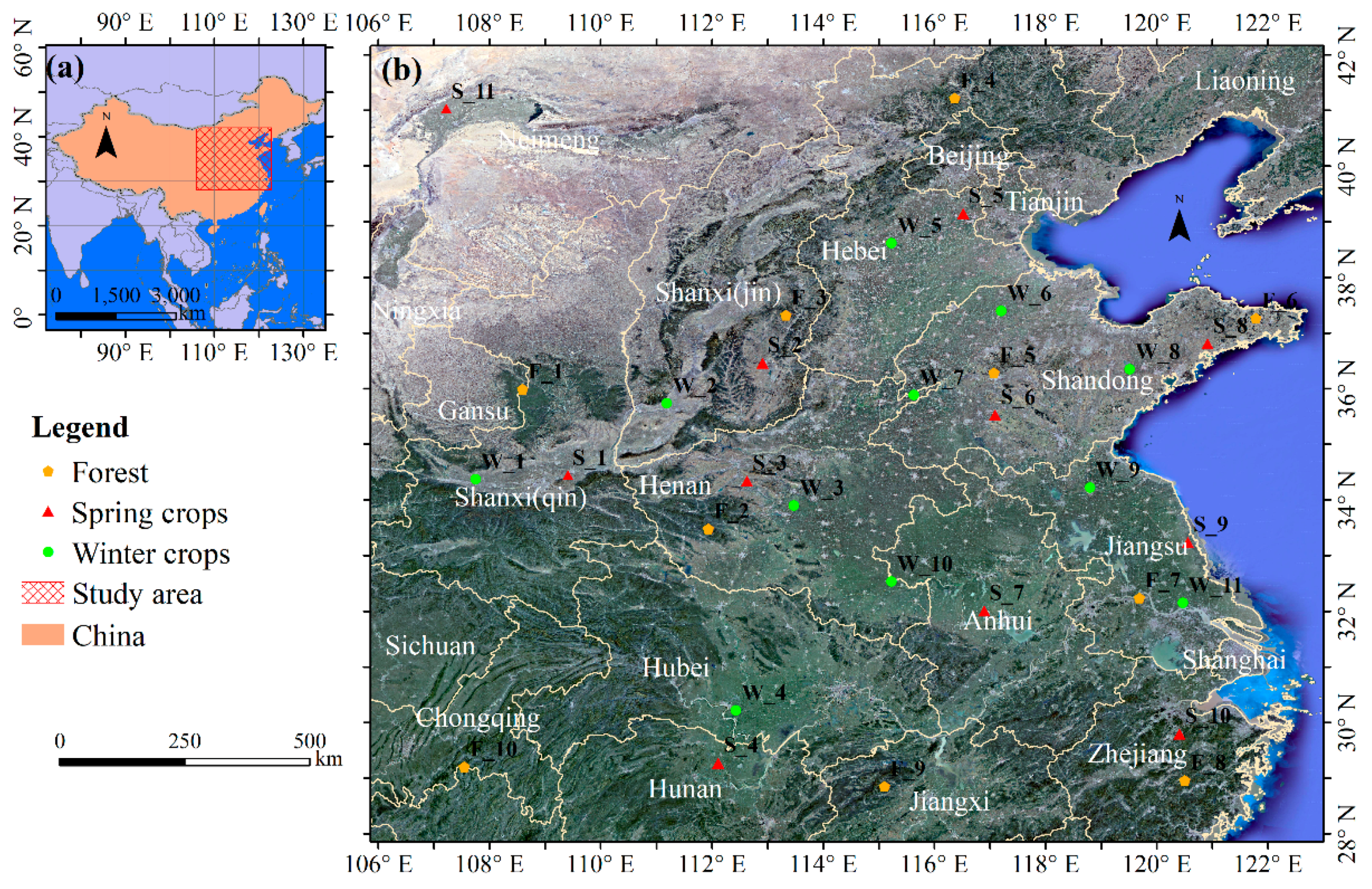These complex environments make agricultural remote sensing challenging in the study area.

3. Materials and Methods

Figure 2 depicts the workflow for the phenology and pixel-based winter crop mapping in the current study. The major modules of work include: (1) Time-window determination for the periods of high and low NDVI for winter crops, based on daily MODIS images, prior knowledge, and multiple trials; (2) construction of composite images: Landsat and Sentinel multi-temporal NDVIs were composited into a new composite image, according to the time-windows; (3) threshold determination derived from a scatter diagram of winter crops and non-winter crops on the composited image, based on some of the samples; and (4) winter crop mapping and validation.

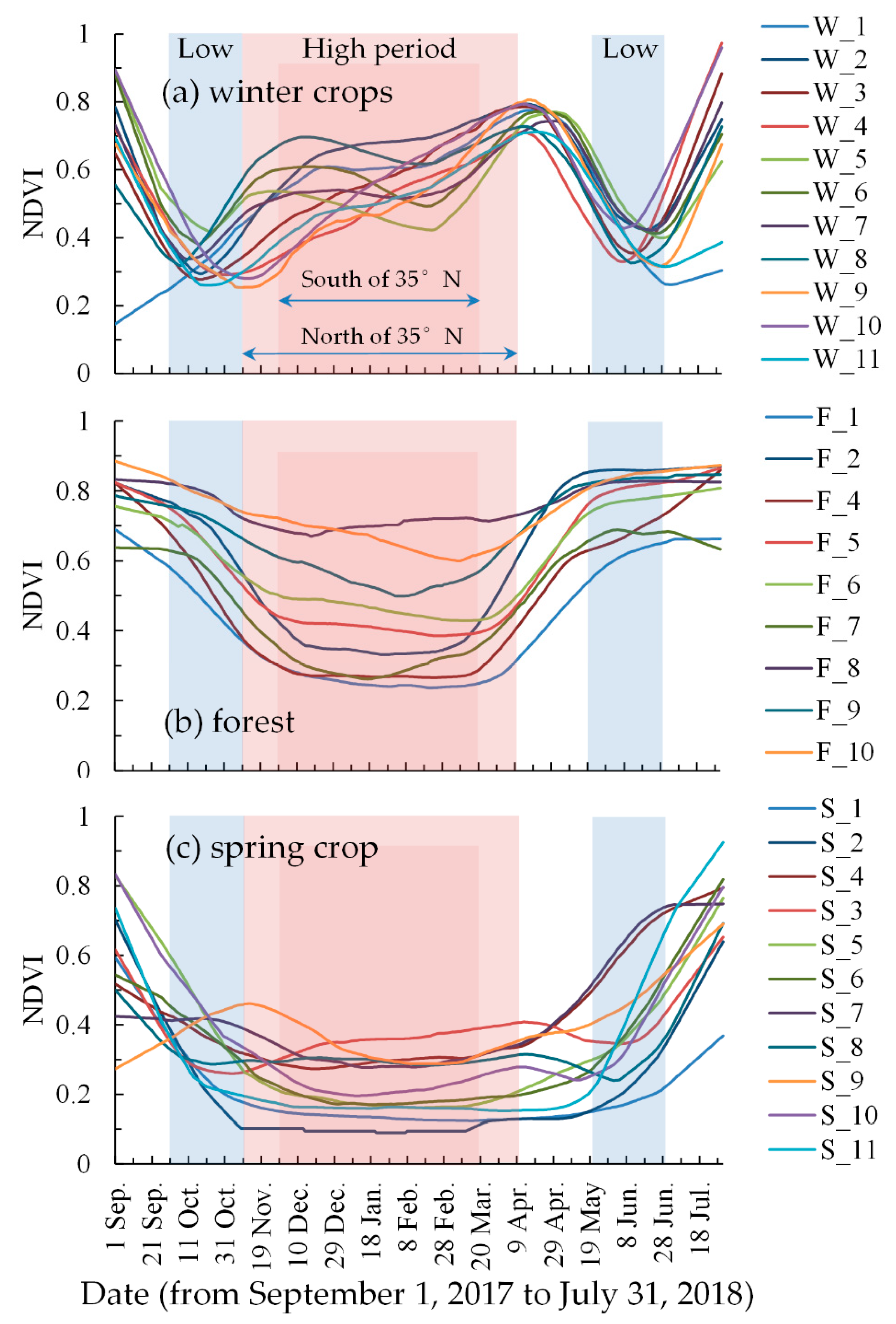
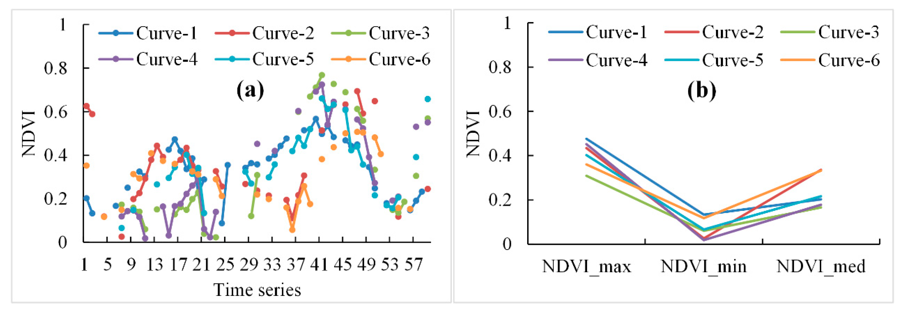
3.1. NDVI Temporal Curves

In order to understand the phenological differences of winter crops in different regions and the phenological difference between winter crops and other surface features, daily MODIS NDVI curves for different sample sites were plotted; the locations and types of these sample sites are plotted in Figure 1. Eleven sample sites of winter crops were selected at random, and these were relatively homogeneously distributed. Each sample site covers 8 × 8 pixels in the MODIS image. The median values of the 64 group values for daily MODIS NDVI were selected to build the phenology curves for each sample site. Similarly, 10 sample sites of forest and 11 sample sites of spring crops were acquired. The MODIS dataset “MODIS/006/MOD13Q1”, with a spatial resolution of 250 m, was implemented in GEE. For each MODIS NDVI time-series curve, there was some missing data due to cloud coverage. Thus, a Lagrange interpolation method was applied to fill in the missing data. In order to smooth the MODIS NDVI time-series curve, a Savitzky–Golay (SG) filter [22,55] was applied, with a window size of 20, in the Origin software (9.1 version). The NDVI is the normalized ratio of the Near Infrared Spectrum (NIR) band to the red band [56,57]:

$$NDVI=\left({\rho }_{NIR}-{\rho }_{red}\right)/\left({\rho }_{NIR}+{\rho }_{red}\right),$$

(1)

where ρ_NIR and ρ_red are the reflectance of the NIR band and the red band, respectively.

While most other crops or types of natural vegetation were harvested or had withered up during December–April, the winter crops were green in color. Thus, the NDVI values of the winter crops were higher than that of other vegetation in this period. During the period of sowing or harvest of winter crops, the NDVI value for the winter crops was less than that of other vegetation types [58]. Consequently, the phenology of winter crops can be characterized by the high and the low values of the NDVI. The low and high NDVI value periods for the winter crops are the key periods for the next step of this work (i.e., the image composite of Landsat and Sentinel imagery). The exact range of the two time-windows (i.e., the low NDVI and high NDVI periods) was identified according to the MODIS NDVI time-series curves and the phenological calendar of winter crops obtained from the official website of the Ministry of Agriculture and Rural Affairs of the People’s Republic of China (http://jiuban.zzys.moa.gov.cn/).

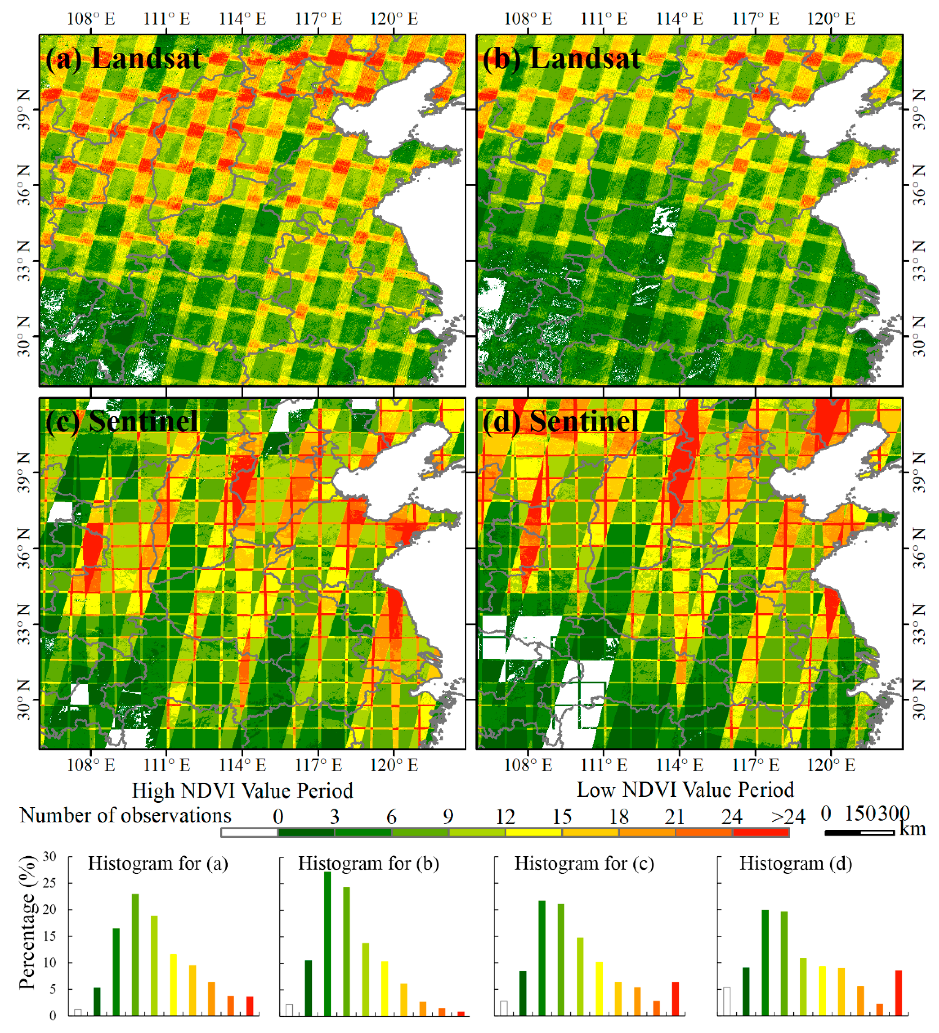
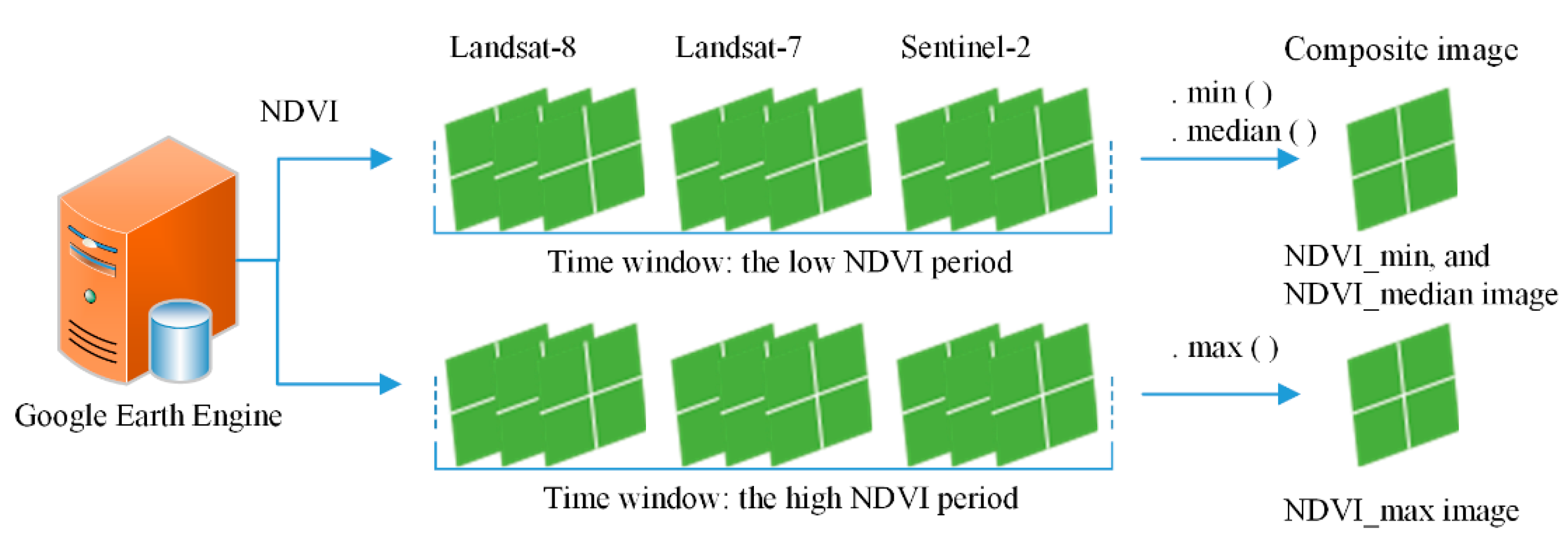
3.2. Composite Landsat and Sentinel Imagery

Landsat and Sentinel imagery have a high spatial-temporal resolution and data quality, and have widely been used in crop-mapping research [59]. The Landsat-7, Landsat-8, and Sentinel-2 image collections of the Google Earth Engine used in the present study were “LANDSAT/LE07/C01/T1_TOA”, “LANDSAT/LC08/C01/T1_TOA”, and “COPERNICUS/S2”, respectively. All images were the top of atmosphere (TOA) reflectance. Landsat and Sentinel-2 TOA data have been widely used for remote sensing monitoring in previous studies [38,60,61]; for example, Dong et al. [41] mapped paddy rice planting areas in northeastern Asia with Landsat-8 TOA images. Additionally, the Google Earth Engine has cloud-mask model codes for Landsat and Sentinel-2 TOA data production and, thus, we can easily remove the pixels which were covered with clouds. More information on the mask cloud model can be found at https://developers.google.com/earth-engine/playground.

The spatial resolution of Landsat images is 30 m, and that of the Sentinel-2 images is 10 m; thus, the spatial resolution of Sentinel-2 was resized to 30 m with a nearest neighbor method. The revisit cycles of the Landsat and Sentinel-2 satellites are 16 days and 10 days, respectively.

First, on a pixel-based scale, the NDVI was computed for each single image from the Landsat-7 and -8 and Sentinel-2 datasets during the low NDVI period. Second, for each pixel location, the minimal NDVI value was selected from all NDVI values, using the “.min()” algorithm of GEE, as shown in Figure 3. All minimal NDVI values were composited into the new NDVI_min image. Then, the NDVI_median image (during the low NDVI period) was obtained in the same way. The NDVI_max image was obtained (during the high NDVI period) using the same method. Thus, for the whole study area, multi-temporal NDVI curves from multi-source images were successfully composited into a three-band image (which we called the composite image) which retained the main characteristics of the winter crops. The specific codes for GEE were shown in Appendix A.

Why was the NDVI_median considered in this study? Due to the influence of cloud shadows, for example, the NDVI_min value of some evergreen forests may be low, similar to that of winter crops. However, the NDVI_median value would be higher than the winter crop classification threshold on the NDVI_median image. Thus, the NDVI_median image avoids misclassification of this type of forest into winter crops, and improves classification accuracy.

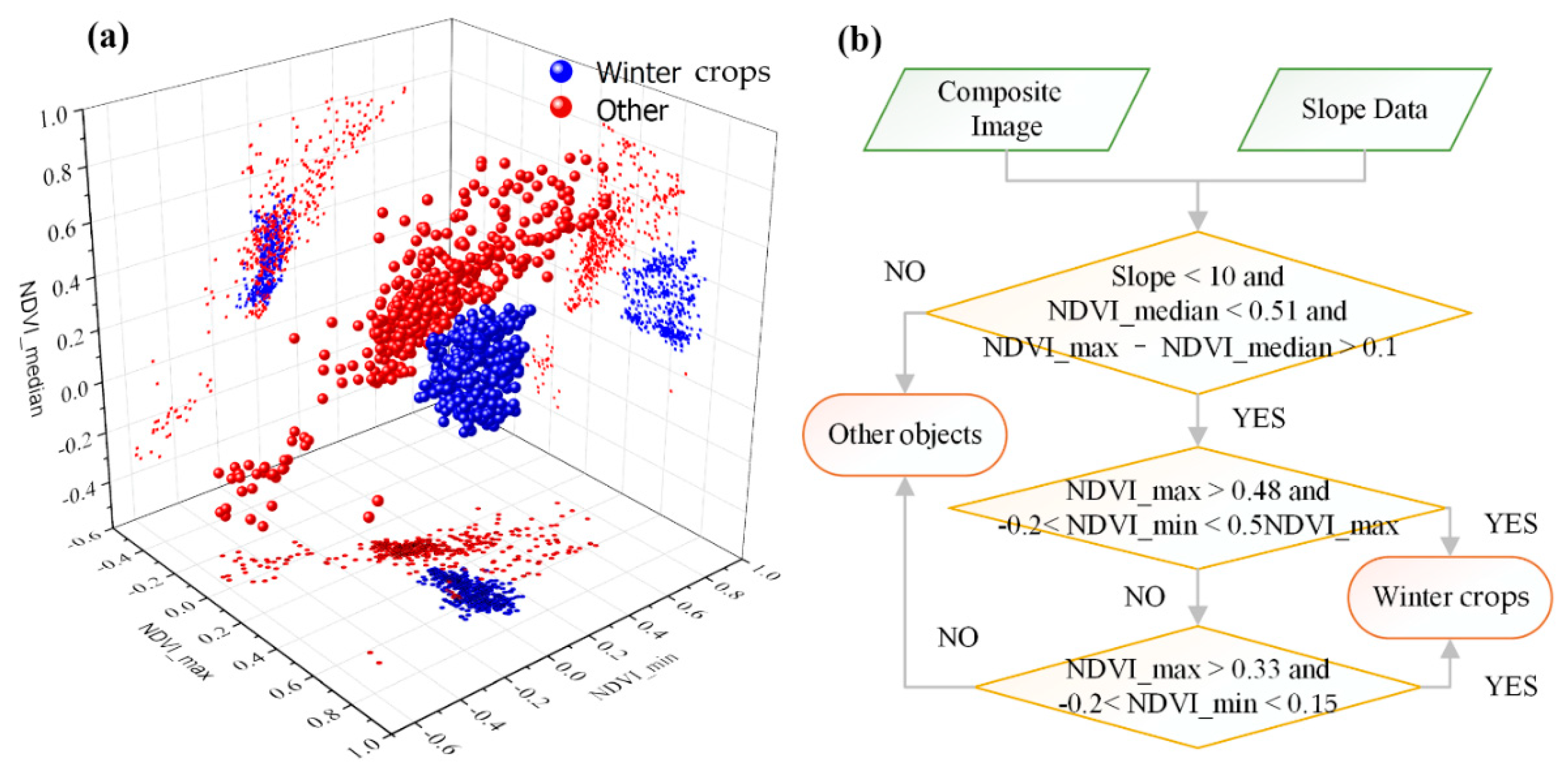
3.3. Decision Tree Classification

The decision tree classifier is a traditional and widely-used classifier in remote sensing classification applications [62,63]. Additionally, it is simple and easy to understand. Therefore, a decision tree classifier was used to map winter crops in the present study. The scatter diagram of winter crops and non-winter crops on the composited image was plotted, based on 625 pixels of non-winter crops and 647 pixels of winter crops, which were randomly selected from the sample sites (Figure 1b). For every sample site, we randomly selected 10–20 pixels based on field survey data. Next, the scatter diagram was used to identify the classification threshold by analyzing and computing the characteristics of objects in the composited image.

To name only a few: Assuming that the minimal value of the winter crops samples is α in the NDVI_max image, the value 10% less than α is the threshold for identifying winter crops in the decision tree (i.e., if a pixel is a winter crop, its value should be more than (1 − 0.1) × α in the NDVI_max image); in the NDVI_min image, assuming that the maximal value of the winter crops samples is β, the value 10% more than β is the threshold for identifying winter crops (i.e., if a pixel is a winter crop, its value should be less than (1 + 0.1) × β in the NDVI_min image). In the present study, the terrain slope was also used to improve the classification accuracy. We empirically defined a terrain slope value less than 10° for winter crops, in accordance with our knowledge of the study area. The slope data source used in this study was “USGS/SRTMGL1_003” in GEE.

3.4. Accuracy Assessment and Amendment of Results

The confusion matrix accuracy assessment approach is a common method to validate classification [64,65,66,67,68]. Thus, the confusion matrix accuracy assessment approach was used to validate the classification result in this paper.

In order to achieve reasonable coverage of the validation samples, 62 blocks of 1 × 1 km² were randomly selected. The sample sites are showed in Figure 1b and their total number is 32. These 32 sample sites were evenly distributed within the study area. This approach could meet the requirement for sample selection [41]. Within 5 km around every sample site, we selected 1–4 blocks. Thus, the validation samples were 62 blocks, each 1 × 1 km². Next, we produced validation data based on these blocks.

First, a Google Earth image was selected as a base map for each block. A Google Earth image with a spatial resolution of 1 m could provide enough information (e.g., colour, texture, and so on) to help us to visually identify the attributes of the surface features, as showed in Figure 4a.

Second, the boundaries of the surface features were plotted, based on the Google Earth image, as in Figure 4b. In the Google Earth image, the boundaries of crops, bare land, water, forest, settlements, and roads were easily identified. Thus, we acquired vector polygons for each surface feature in every block.

Third, the attributes of the vector polygons were identified and labelled by field-based survey data, as in Figure 4c. All other objects, except for the winter crops, were labelled as “Other” type.

Fourth, these vector polygons with attribute information were converted into raster data with a spatial resolution of approximately 3 m, as in Figure 4d. This raster data was validation data and was regarded as ground truth data, due to the high spatial resolution and accurate feature boundaries.

The theory and methodology of confusion matrix accuracy assessment are shown below.

First, the error confusion matrix of the sample was constructed, as shown in

Table 1. Error confusion matrix of sample counts and estimated area proportion.

(a) Error Matrix of Sample Counts (Unit, Pixel)							(b) Error Matrix of Estimated Area Proportion
	j	1	2	…	q	Total		j	1	2	…	q	Total
i							i
1		n11	n12	…	n1q	n1•	1		p11	p12	…	p1q	p1•
2		n21	n22	…	n2q	n2•	2		p21	p22	…	p2q	p2•
⁞		⁞	⁞	⁞	⁞	⁞	⁞		⁞	⁞	⁞	⁞	⁞
q		nq1	nq2	…	nqq	nq•	q		pq1	pq2	…	pqq	pq•
Total		n•1	n•2	…	n•q	n	Total		p•1	p•2	…	p•q	1

Map categories are the rows and validation categories are the columns.

a. The map categories (i = 1, 2, …, q) are represented by rows and the validation categories (j = 1, 2, …, q) by columns in Table 1.

The error matrix of the estimated area proportion is computed and plotted in Table 1b, according to the following equation [68,69]:

$$p_{ij}=w_i\times \left(n_{ij}/n_{i\cdot }\right),$$

(2)

$$w_i=A_i/A_{tot},$$

(3)

where n_ij represents the corresponding value in Table 1a; n_i• represents the total of the rows i in Table 1a; w_i represents the weight of the area mapped for category i taking into account the total area of the sample; A_i represents the sample area of category i; and A_tot represents the total area of the sample.

Then, the user accuracy (U) and producer accuracy (P) for any map category, overall accuracy (O), and Kappa coefficient (K) can be estimated directly from Table 1b, according to the following equations [68,69]:

$$U_i=p_{ii}/p_{i\cdot },$$

(4)

$$S\left(U_i\right)={\left\{p_{ii}{p}_{i\cdot }{}^{-4}\left[p_{ii}{\displaystyle \sum _{j\ne i}^q{p}_{ij}\frac{w_j-p_{ij}}{w_{j}n}}+\frac{\left(w_i-p_{ii}\right){\left(p_{i\cdot }-p_{ii}\right)}^2}{w_{i}n}\right]\right\}}^{0.5},$$

(5)

$$P_j=p_{jj}/p_{\cdot j},$$

(6)

$$S\left(P_j\right)={\left[p_{jj}\left(w_j-p_{jj}\right)/\left(w_j{}^{3}n\right)\right]}^{0.5},$$

(7)

$$O={\displaystyle \sum _{j=1}^q{p}_{jj}},$$

(8)

$$S\left(O\right)={\left[{\displaystyle \sum _{i=1}^q{p}_{ii}\left(w_i-p_{ii}\right)}/\left(w_{i}n\right)\right]}^{0.5},$$

(9)

$$K=\left[n\times {\displaystyle \sum _{i=1}^q{n}_{ii}}-{\displaystyle \sum _{i=1}^q\left(n_{i\cdot }\times n_{\cdot i}\right)}\right]/\left[n^2-{\displaystyle \sum _{i=1}^q\left(n_{i\cdot }\times n_{\cdot i}\right)}\right],$$

(10)

where S(U_i), S(P_j), and S(O) are the standard error of the user accuracy, producer accuracy, and overall accuracy, respectively.

The adjusted area of mapped category j is computed according to the following equation:

$$A_{a,j}=A_{m,j}\times \left(1+U_j-P_j\right),$$

(11)

where A_a,j represents the adjusted area of mapped category j; the subscript a denotes “adjusted”; and A_m,j represents the original mapped area of category j.

3.5. Comparison Relative to MODIS Classification

In order to characterize the effectiveness of a coarser spatial resolution for mapping winter crops in the study area, MODIS datasets were utilized to map winter crops using the same classification method. The MODIS dataset used in the present study was “MODIS/006/MOD13Q1” in GEE, with a spatial resolution of 250 m. The accuracy validation methods were the same as described above.

4. Results

4.1. Determination of the Time-Window

As shown in Figure 5, there was a significant difference between the NDVI curves of the winter crops and those of other vegetation. The NDVI curves of forest and spring crops exhibited a wide mouthed “U” shape, while the winter crop NDVI curves exhibited a “W” shape. There were some differences in the winter crop NDVI curves in different regions, although their trends were similar. The samples W_3, W_4, W_9, W_10, and W_11 differed from other winter crop samples in November and December, as shown in Figure 5a. The samples W_3, W_4, W_9, W_10, and W_11 were distributed south of 35°N in the study area. For the part north of 35°N, the winter crop sowing date is later than that of south of 35°N, and the wilting time of other vegetation is earlier than that of south of 35°N. This result is consistent with previous studies [58,70]. Thus, the study area was divided into two sub-parts, based on the line 35°N: One part north of 35°N, and another part south of 35°N.

According to results of previous studies [58,70], our prior knowledge, and multiple trials, we designed a time-window for the composite NDVI time-series curves as the following:

For the part north of 35°N, the low NDVI value period was defined as 1 October to 10 November 2017 and 20 May to 30 June 2018; and the high NDVI value period was defined as 11 November to 10 April 2018, as in Figure 5.

For the part south of 35°N, the low NDVI value period was the same as that of the north part; the high NDVI value period was defined as 1 December to 20 March 2018.

4.2. Thresholds for Winter Crops Mapping

Figure 6a shows the characteristics of winter crops and other surface features in the composite image. This figure shows that there are significant differences between winter crops and non-winter crops in the composite image. The specific algorithm used to extract winter crops is shown in Figure 6b. In the first layer of the decision tree for winter crop classification, the slope value should be less than 10°; in the NDVI_median image, the value of winter crops should be less than 0.51; and the difference between NDVI_max and NDVI_median should be more than 0.1. If a pixel is a winter crop, it must meet these three primary constraint conditions.

In the second layer of the decision tree model, if a pixel a winter crop, its NDVI_max value should be more than 0.48 and should be more than double its NDVI_min value. At the same time, the NDVI_min value should be more than −0.2. Otherwise, the pixel enters the third judgement layer of the decision tree model. If its NDVI_min value is less than 0.15 and more than −0.2, and its NDVI_max value is more than 0.33, it would be classified as a winter crop; otherwise, it would be classified into another category.

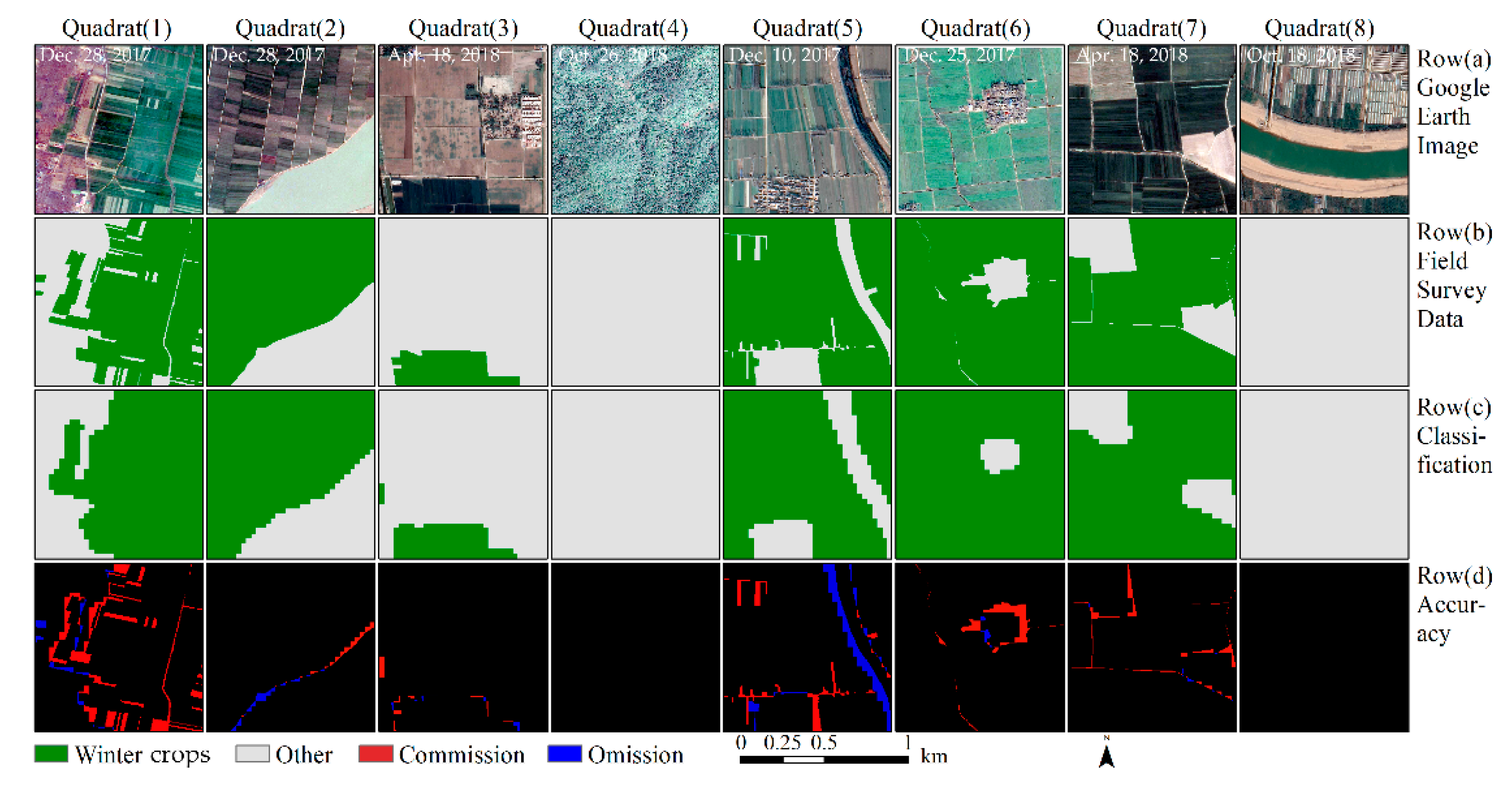
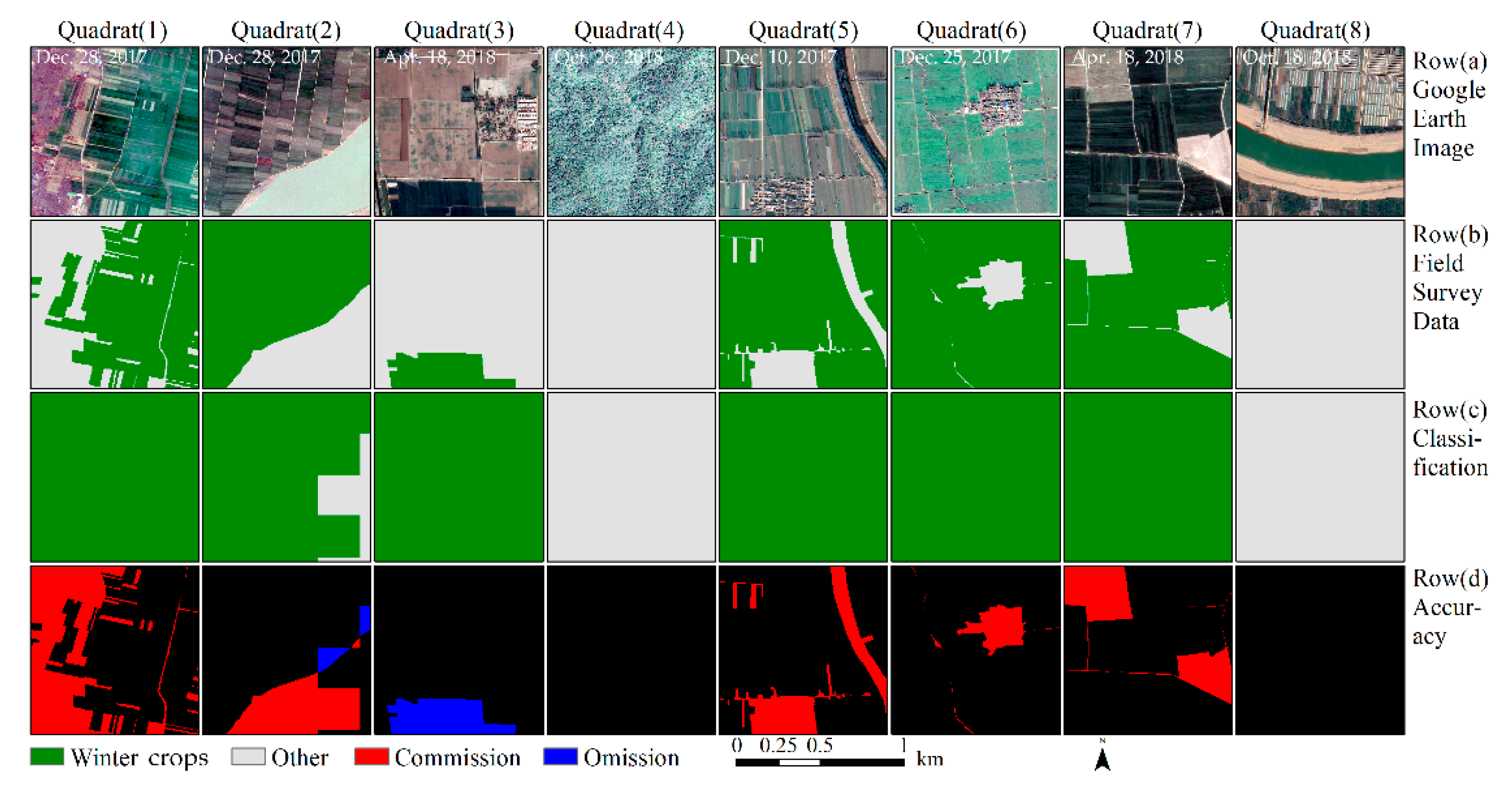
4.3. Classification and Accuracy Assessment

The classification results for winter crops are plotted in Figure 7. The total area of winter crops in the study area was 201,673 km², with an adjusted area of 207,641 km². Figure 7 shows the spatial distribution of winter crops. For longitude, the range of 112° to 121° was the major distribution region of winter crops, accounting for 92% of the total area of winter crops in the study area (see Figure 7b). For latitude, the range of 32° to 38° was the major distribution region of winter crops, accounting for 85% of the total area of winter crops in the study area (see Figure 7c). For altitude, about 93% of winter crops were distributed below 150 m (see Figure 7d).

The overall classification accuracy was 96.22%, with a kappa coefficient of 0.93 (see

Table 2. Results of accuracy validation for the composite image classification.

Class	Error matrix (Pixel/Proportion)			Accuracy (%)
	Winter Crops	Other	Total	User’s	Producer’s	Overall
Winter Crops	2,306,862/0.6125	39,260/0.0104	2,346,122/0.6229	98.32 ± 0.016	95.57 ± 0.016	96.22 ± 0.019
Other	107,042/0.0264	1,421,836/0.3507	1,528,878/0.3771	93.00 ± 0.039	97.11 ± 0.041
Total	2,413,904/0.6389	1,461,096/0.3611	3,875,000/1.0000	/	/	/

). For winter crops, the user and producer accuracies were 98.32% and 95.57%, respectively; demonstrating that winter crops were accurately extracted in the study area.

In order to better prove the credibility of the accuracy validation, public data (http://www.stats.gov.cn/tjsj/ndsj/2018/indexch.htm) from the Chinese government in 2017 was compared with our classification results at a provincial scale, as shown in

Table 3. Compared with public data at a provincial scale (km²).

Province	Henan	Shandong	Anhui	Jiangsu	Hebei	Hubei	Shanxi(qin)	Total
Public data	58,703	40,919	31,769	25,881	23,979	21,244	11,427	213,922
Classification	55,869	42,689	31,604	28,371	22,155	9803	5509	196,001
Error (%)	4.83	4.33	0.52	9.62	7.61	53.85	51.79	8.38

The year of public data and the classification data is 2017 and 2018, respectively.

. For the main production provinces (i.e., Henan, Shandong, and Anhui provinces), the classification data approximates the public data. In the Hubei and Shanxi(qin) provinces, the classification data is about half of the public data.

Figure 8 intuitively describes the results of the accuracy assessment. The edge of the winter crop plots are the primary region for classification errors. Some minor linear objects (e.g., paths and creeks) are easily misclassified as winter crops.

4.4. Classification Results for MODIS

For the MODIS images with a spatial resolution of 250 m, the overall accuracy was 82.11% and the kappa coefficient was 0.57 (see

Table 4. Results of accuracy validation for MODIS classification.

Class	Error matrix (Pixel/Proportion)			Accuracy (%)
	Winter Crops	Other	Total	User’s	Producer’s	Overall
Winter Crops	2,228,950/0.4903	636,618/0.1343	2,865,568/0.6046	77.78 ± 0.039	91.34 ± 0.053	82.11 ± 0.037
Other	113,800/0.0446	895,632/0.3508	1,009,432/0.3954	88.73 ± 0.046	72.32 ± 0.050
Total	2,342,750/0.5148	1,532,250/0.4851	3,875,000/1.0000	/	/	/

), 14.11% less than the 96.22% accuracy derived from the composite images. Further, the user and producer accuracies of the winter crops were 77.78% and 91.34%, respectively. Figure 9 shows that the MODIS images were hardly able to identify villages, rivers, and roads; these were often misclassified as winter crops. The area classified as winter crops was 263,168 km², based on the MODIS images, with an adjusted area of 227,489 km².

5. Discussion

Although the MODIS images can provide daily observations for characterizing the phenology of winter crops well, their coarse spatial resolution can hardly accurately identify winter crops in China. As the field size of most farmland in China is smaller than a MODIS pixel (250 × 250 m²), village and spring-seeding farmland can be misclassified into winter crops, which has been reported by Qiu et al. [2]. With the Landsat or Sentinel-2 images, we can’t accurately identify winter crops in the entire study area too; the reason being that there are not enough available images to provide dense observations in the temporal dimension due to the revisit time and the influence of cloudy weather in some regions. Figure 10 suggests that the number of observations are less than three in most regions of southwestern part of the study area, making it almost impossible to identify winter crops in accordance with our experiment. In single-scene image-overlapped regions, the observation numbers are more than 12. Therefore, it is necessary to integrate the Landsat and Sentinel-2 images in this study.

With the identification of the low NDVI value and high NDVI value periods in the whole growth cycle of winter crops and the computation of the minimal and maximal NDVI values, this algorithm is promising for mapping winter crops in large areas. While Sun et al. [22] proposed a vegetation index curve shape-based algorithm to classify crops, it was difficult to obtain almost-complete and similar vegetation index curves from Landsat and Sentinel-2 images in the study area. For the original time-series NDVI of winter crops, derived from Sentinel-2 and Landsat-7 and -8 images, there were many different shapes of NDVI curves for winter crop fields, which were caused by the differences in phenology, image acquisition date, and number of non-cloudy observations, as well as weather conditions. These differences may have reduced the accuracy of the classification. For instance, if one type of NDVI curve was omitted in the sample dataset, relevant winter crops may not have been identified. The composited NDVI curves avoided this problem (Figure 11). Further, the phenology differences of winter crops in different regions [2] and the intra-class variability of NDVI [71] could be removed.

Although this proposed method is a promising solution for winter crop mapping, the number of observations is still an issue for characterizing the phenology of winter crops. The Chinese GaoFen satellite [72] has a revisit cycle of four days, and provides high frequency images with low cost; if the GEE data catalog included images from this satellite, the risk of missing images would be reduced. Also, several types of supplementary data sets could be adopted in the winter crop classification, such as agro-meteorological data [73] and/or cropland data [2]. Provided that this supplementary information is reliable, it could have tremendous potential for improving classification accuracy and efficiency [2,74]. As an example, there were some commission errors for the winter crop map in some minor patches and edges of villages (Figure 8), and these classification errors could be reduced if a farmland mask was applied. Although we obtained a high classification accuracy for winter crops, we still need to further optimize the classification model to distinguish winter crops, such as winter rapeseed and winter garlic.

The classification data for the Hubei and Shanxi(qin) provinces is about half as accurate as the public data. For the Hubei province, the areas of many terraces are generally less than 1 km², which is very fragmented when compared with the remote sensing images in this study. Thus, some winter crops were not accurately identified in the remote sensing images. Additionally, in some regions, there were no available images, due to the influence of cloudy weather. These two reasons may be able to answer why our classification data had less area than the public data for the Hubei province. For the Shanxi(qin) province, we found the phenomenon that nursery stock and winter crops are interplanted in some regions in our field survey. For this planting structure, our classification method did not accurately identify winter crops. Additionally, the area of winter crops has been decreasing since 2000, according to public data for the Shanxi(qin) province. The public data may also have had some errors compared with the truth data, which may be another reason for explaining that our classification data for the Shanxi(qin) province was inconsistent with the public data.

6. Conclusions

Existing research on large-scale winter crop mapping has generally focused on using highly temporal MODIS datasets. However, our knowledge of the new distribution of winter crops in China remains limited. In order to resolve the issue, we proposed an algorithm which composites the multi-temporal NDVI for rapidly mapping winter crop planting areas using Landsat-7 and -8 and Sentinel-2 optical images. We have achieved the following findings:

(1)

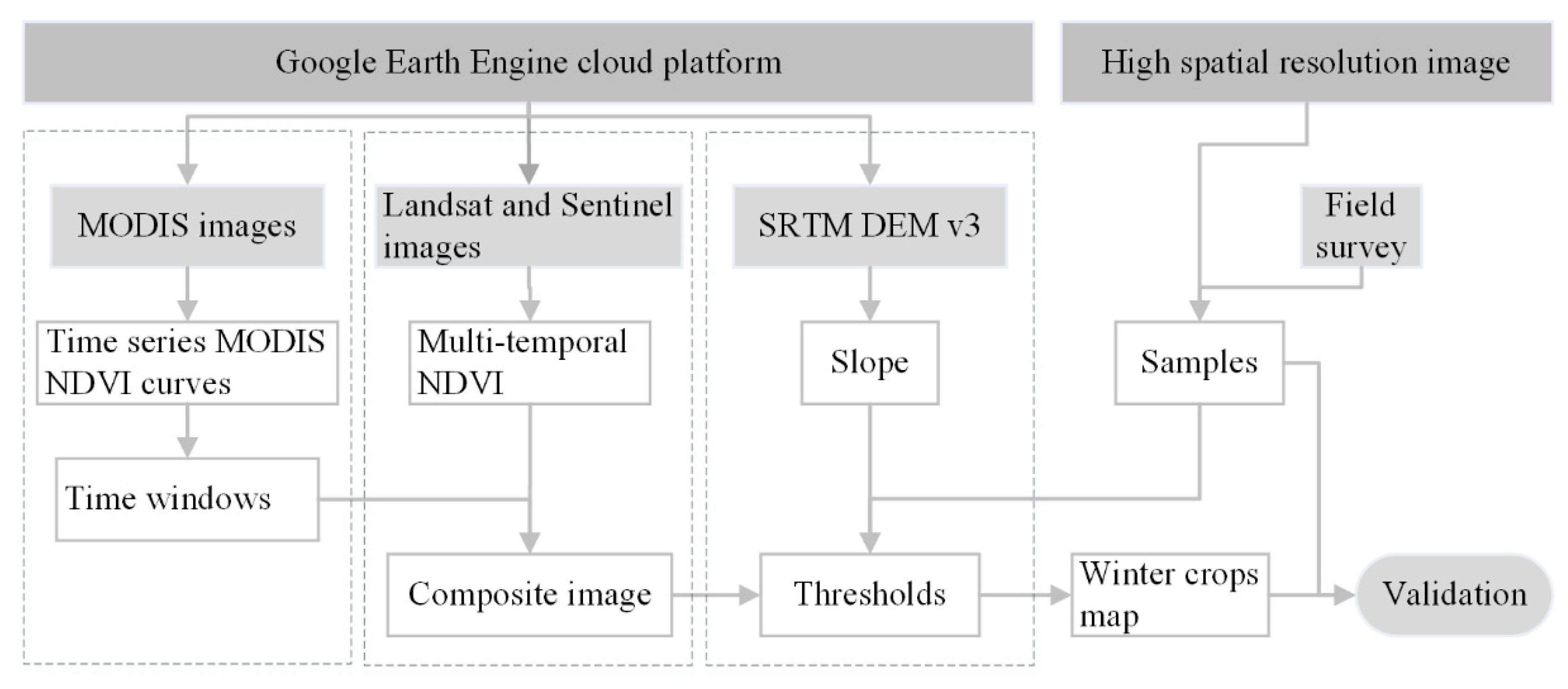
The composited algorithm composites the multi-temporal NDVI from Landsat-7 and -8 and Sentinel-2 optical images into three key values, according to two time-windows, a period of low NDVI values and a period of high NDVI values, for winter crops. In the period of high NDVI value, a max NDVI image was obtained from the multi-temporal NDVI. In the period of low NDVI value, min and median NDVI images were obtained from the multi-temporal NDVI. Thus, the three images are the composited image in this study.

(2)

The time-series NDVI composited algorithm can reduce the differences in winter crop phenologies caused by differences in sowing time and satellite imaging time. This approach reduces the demand on the number of available images required for mapping and is robust for mapping winter crops in Northern China. The results reported here are sufficient to satisfy the accuracy requirements for winter crop mapping on a large scale.

(3)

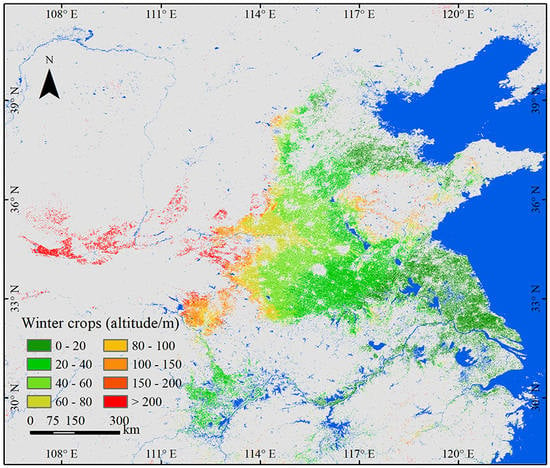
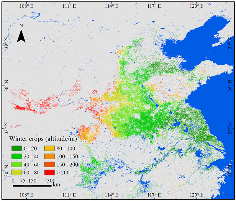
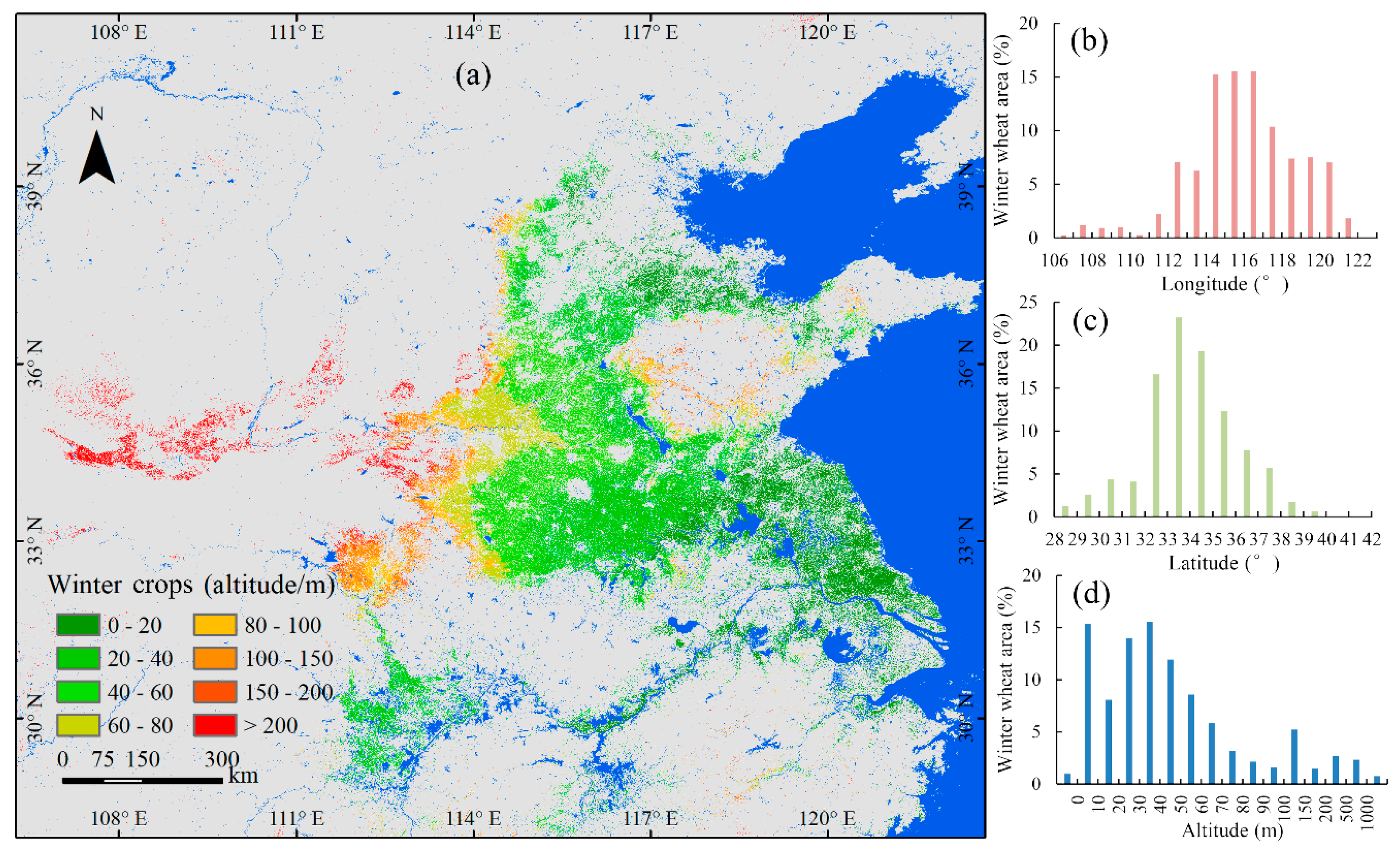
This study generated an accurate winter crop map of Northern China in 2018, with a spatial resolution of 30 m, using a decision tree classification method. The overall accuracy is 96%, with a kappa coefficient of 0.93.

(4)

The Google Earth Engine cloud platform has powerful data storage and management capabilities and data processing capabilities, providing a technical means for the wide spatial and temporal scales of remote sensing mapping studies. The effective implementation of this approach, proposed in this paper, over a large area is primarily attributed to the utility of the Google Earth Engine’s cloud-computing technology; these findings showcase the tremendous potential of this technology for mapping winter crops at a global scale.

References

- Xie, Y.; Wang, P.X.; Bai, X.J.; Khan, J.; Zhang, S.Y.; Li, L.; Wang, L. Assimilation of the leaf area index and vegetation temperature condition index for winter wheat yield estimation using Landsat imagery and the ceres-wheat model. Agric. For. Meteorol. 2017, 246, 194–206. [Google Scholar] [CrossRef]
- Qiu, B.W.; Luo, Y.H.; Tang, Z.H.; Chen, C.C.; Lu, D.F.; Huang, H.Y.; Chen, Y.Z.; Chen, N.; Xu, W.M. Winter wheat mapping combining variations before and after estimated heading dates. ISPRS J. Photogramm. Remote Sens. 2017, 123, 35–46. [Google Scholar] [CrossRef]
- Liu, J.T.; Feng, Q.L.; Gong, J.H.; Zhou, J.P.; Liang, J.M.; Li, Y. Winter wheat mapping using a random forest classifier combined with multi-temporal and multi-sensor data. Int. J. Digit. Earth 2018, 11, 783–802. [Google Scholar] [CrossRef]
- Huang, J.X.; Ma, H.Y.; Sedano, F.; Lewis, P.; Liang, S.; Wu, Q.L.; Su, W.; Zhang, X.D.; Zhu, D.H. Evaluation of regional estimates of winter wheat yield by assimilating three remotely sensed reflectance datasets into the coupled wofost-prosail model. Eur. J. Agron. 2019, 102, 1–13. [Google Scholar] [CrossRef]
- Huang, J.X.; Sedano, F.; Huang, Y.B.; Ma, H.Y.; Li, X.L.; Liang, S.L.; Tian, L.Y.; Zhang, X.D.; Fan, J.L.; Wu, W.B. Assimilating a synthetic kalman filter leaf area index series into the wofost model to improve regional winter wheat yield estimation. Agric. For. Meteorol. 2016, 216, 188–202. [Google Scholar] [CrossRef]
- Huang, J.X.; Tian, L.Y.; Liang, S.L.; Ma, H.Y.; Becker-Reshef, I.; Huang, Y.B.; Su, W.; Zhang, X.D.; Zhu, D.H.; Wu, W.B. Improving winter wheat yield estimation by assimilation of the leaf area index from Landsat TM and MODIS data into the wofost model. Agric. For. Meteorol. 2015, 204, 106–121. [Google Scholar] [CrossRef]
- Nasrallah, A.; Baghdadi, N.; Mhawej, M.; Faour, G.; Darwish, T.; Belhouchette, H.; Darwich, S. A novel approach for mapping wheat areas using high resolution Sentinel-2 images. Sensors 2018, 18, 2089. [Google Scholar] [CrossRef] [PubMed]
- Hao, Z.; Zhao, H.L.; Zhang, C.; Wang, H.; Jiang, Y.Z.; Yi, Z.Y. Estimating winter wheat area based on an SVM and the variable fuzzy set method. Remote Sens. Lett. 2019, 10, 343–352. [Google Scholar] [CrossRef]
- Zhang, L.L.; Feng, H.; Dong, Q.G.; Jin, N.; Zhang, T.L. Mapping irrigated and rainfed wheat areas using high spatial-temporal resolution data generated by Moderate Resolution Imaging Spectroradiometer and Landsat. J. Appl. Remote Sens. 2018, 12, 046023. [Google Scholar] [CrossRef]
- Ma, H.Q.; Jing, Y.S.; Huang, W.J.; Shi, Y.; Dong, Y.Y.; Zhang, J.C.; Liu, L.Y. Integrating early growth information to monitor winter wheat powdery mildew using multi-temporal Landsat-8 imagery. Sensors 2018, 18, 3290. [Google Scholar] [CrossRef] [PubMed]
- Atzberger, C. Advances in remote sensing of agriculture: Context description, existing operational monitoring systems and major information needs. Remote Sens. 2013, 5, 949–981. [Google Scholar] [CrossRef]
- Friedl, M.A.; Sulla-Menashe, D.; Tan, B.; Schneider, A.; Ramankutty, N.; Sibley, A.; Huang, X.M. MODIS collection 5 global land cover: Algorithm refinements and characterization of new datasets. Remote Sens. Environ. 2010, 114, 168–182. [Google Scholar] [CrossRef]
- Bartholome, E.; Belward, A.S. Glc2000: A new approach to global land cover mapping from earth observation data. Int. J. Remote Sens. 2005, 26, 1959–1977. [Google Scholar] [CrossRef]
- Dong, J.W.; Xiao, X.M.; Kou, W.L.; Qin, Y.W.; Zhang, G.L.; Li, L.; Jin, C.; Zhou, Y.T.; Wang, J.; Biradar, C.; et al. Tracking the dynamics of paddy rice planting area in 1986–2010 through time-series Landsat images and phenology-based algorithms. Remote Sens. Environ. 2015, 160, 99–113. [Google Scholar] [CrossRef]
- Siyal, A.A.; Dempewolf, J.; Becker-Reshef, I. Rice yield estimation using Landsat ETM plus data. J. Appl. Remote Sens. 2015, 9, 095986. [Google Scholar] [CrossRef]
- Ma, Y.P.; Wang, S.L.; Zhang, L.; Hou, Y.Y.; Zhuang, L.W.; He, Y.B.; Wang, F.T. Monitoring winter wheat growth in north china by combining a crop model and remote sensing data. Int. J. Appl. Earth Obs. Geoinf. 2008, 10, 426–437. [Google Scholar]
- Dominguez, J.A.; Kumhalova, J.; Novak, P. Winter oilseed rape and winter wheat growth prediction using remote sensing methods. Plant Soil Environ. 2015, 61, 410–416. [Google Scholar]
- He, L.; Song, X.; Feng, W.; Guo, B.B.; Zhang, Y.S.; Wang, Y.H.; Wang, C.Y.; Guo, T.C. Improved remote sensing of leaf nitrogen concentration in winter wheat using multi-angular hyperspectral data. Remote Sens. Environ. 2016, 174, 122–133. [Google Scholar] [CrossRef]
- Franke, J.; Menz, G. Multi-temporal wheat disease detection by multi-spectral remote sensing. Precis. Agric. 2007, 8, 161–172. [Google Scholar] [CrossRef]
- Tian, H.F.; Wu, M.Q.; Wang, L.; Niu, Z. Mapping early, middle and late rice extent using Sentinel-1A and Landsat-8 data in the poyang lake plain, China. Sensors 2018, 18, 185. [Google Scholar] [CrossRef]
- Tao, J.B.; Wu, W.B.; Zhou, Y.; Wang, Y.; Jiang, Y. Mapping winter wheat using phenological feature of peak before winter on the north china plain based on time-series MODIS data. J. Integr. Agric. 2017, 16, 348–359. [Google Scholar] [CrossRef]
- Sun, H.S.; Xu, A.G.; Lin, H.; Zhang, L.P.; Mei, Y. Winter wheat mapping using temporal signatures of MODIS vegetation index data. Int. J. Remote Sens. 2012, 33, 5026–5042. [Google Scholar] [CrossRef]
- Pan, Y.Z.; Li, L.; Zhang, J.S.; Liang, S.L.; Zhu, X.F.; Sulla-Menashe, D. Winter wheat area estimation from MODIS-EVI time-series data using the crop proportion phenology index. Remote Sens. Environ. 2012, 119, 232–242. [Google Scholar] [CrossRef]
- Chu, L.; Liu, Q.S.; Huang, C.; Liu, G.H. Monitoring of winter wheat distribution and phenological phases based on MODIS time-series: A case study in the yellow river delta, china. J. Integr. Agric. 2016, 15, 2403–2416. [Google Scholar] [CrossRef]
- Ahmadian, N.; Ghasemi, S.; Wigneron, J.P.; Zolitz, R. Comprehensive study of the biophysical parameters of agricultural crops based on assessing Landsat 8 OLI and Landsat 7 ETM+ vegetation indices. Gisci. Remote Sens. 2016, 53, 337–359. [Google Scholar] [CrossRef]
- Ozelkan, E.; Chen, G.; Ustundag, B.B. Multiscale object-based drought monitoring and comparison in rainfed and irrigated agriculture from Landsat 8 OLI imagery. Int. J. Appl. Earth Obs. Geoinf. 2016, 44, 159–170. [Google Scholar] [CrossRef]
- Bolyn, C.; Michez, A.; Gaucher, P.; Lejeune, P.; Bonnet, S. Forest mapping and species composition using supervised per pixel classification of Sentinel-2 imagery. Biotechnol. Agron. Soc. Environ. 2018, 22, 172–187. [Google Scholar]
- Sonobe, R.; Yamaya, Y.; Tani, H.; Wang, X.F.; Kobayashi, N.; Mochizuki, K. Crop classification from Sentinel-2-derived vegetation indices using ensemble learning. J. Appl. Remote Sens. 2018, 12, 026019. [Google Scholar] [CrossRef]
- Belgiu, M.; Csillik, O. Sentinel-2 cropland mapping using pixel-based and object-based time-weighted dynamic time warping analysis. Remote Sens. Environ. 2018, 204, 509–523. [Google Scholar] [CrossRef]
- Lu, L.Z.; Tao, Y.; Di, L.P. Object-based plastic-mulched landcover extraction using integrated Sentinel-1 and Sentinel-2 data. Remote Sens. 2018, 10, 1820. [Google Scholar] [CrossRef]
- Zheng, Q.; Huang, W.J.; Cui, X.M.; Shi, Y.; Liu, L.Y. New spectral index for detecting wheat yellow rust using Sentinel-2 multispectral imagery. Sensors 2018, 18, 868. [Google Scholar] [CrossRef] [PubMed]
- Alonso, A.; Munoz-Carpena, R.; Kennedy, R.E.; Murcia, C. Wetland landscape spatio-temporal degradation dynamics using the new Google Earth Engine cloud-based platform: Opportunities for non-specialists in remote sensing. Trans. ASABE 2016, 59, 1333–1344. [Google Scholar]
- Xiong, J.; Thenkabail, P.S.; Gumma, M.K.; Teluguntla, P.; Poehnelt, J.; Congalton, R.G.; Yadav, K.; Thau, D. Automated cropland mapping of continental africa using Google Earth Engine cloud computing. ISPRS J. Photogramm. Remote Sens. 2017, 126, 225–244. [Google Scholar] [CrossRef]
- Chen, F.; Zhang, M.M.; Tian, B.S.; Li, Z. Extraction of glacial lake outlines in Tibet Plateau using Landsat 8 imagery and Google Earth Engine. IEEE J. Sel. Top. Appl. Earth Obs. Remote Sens. 2017, 10, 4002–4009. [Google Scholar] [CrossRef]
- Teluguntla, P.; Thenkabail, P.S.; Oliphant, A.; Xiong, J.; Gumma, M.K.; Congalton, R.G.; Yadav, K.; Huete, A. A 30-m Landsat-derived cropland extent product of australia and china using random forest machine learning algorithm on Google Earth Engine cloud computing platform. ISPRS J. Photogramm. Remote Sens. 2018, 144, 325–340. [Google Scholar] [CrossRef]
- Gorelick, N.; Hancher, M.; Dixon, M.; Ilyushchenko, S.; Thau, D.; Moore, R. Google Earth Engine: Planetary-scale geospatial analysis for everyone. Remote Sens. Environ. 2017, 202, 18–27. [Google Scholar] [CrossRef]
- Campos-Taberner, M.; Moreno-Martinez, A.; Garcia-Haro, F.J.; Camps-Valls, G.; Robinson, N.P.; Kattge, J.; Running, S.W. Global estimation of biophysical variables from Google Earth Engine platform. Remote Sens. 2018, 10, 1167. [Google Scholar] [CrossRef]
- Traganos, D.; Aggarwal, B.; Poursanidis, D.; Topouzelis, K.; Chrysoulakis, N.; Reinartz, P. Towards global-scale seagrass mapping and monitoring using Sentinel-2 on Google Earth Engine: The case study of the aegean and ionian seas. Remote Sens. 2018, 10, 1227. [Google Scholar] [CrossRef]
- Tsai, Y.H.; Stow, D.; Chen, H.L.; Lewison, R.; An, L.; Shi, L. Mapping vegetation and land use types in fanjingshan national nature reserve using Google Earth Engine. Remote Sens. 2018, 10, 927. [Google Scholar] [CrossRef]
- Hansen, M.C.; Potapov, P.V.; Moore, R.; Hancher, M.; Turubanova, S.A.; Tyukavina, A.; Thau, D.; Stehman, S.V.; Goetz, S.J.; Loveland, T.R.; et al. High-resolution global maps of 21st-century forest cover change. Science 2013, 342, 850–853. [Google Scholar] [CrossRef]
- Dong, J.W.; Xiao, X.M.; Menarguez, M.A.; Zhang, G.L.; Qin, Y.W.; Thau, D.; Biradar, C.; Moore, B. Mapping paddy rice planting area in northeastern asia with Landsat 8 images, phenology-based algorithm and Google Earth Engine. Remote Sens. Environ. 2016, 185, 142–154. [Google Scholar] [CrossRef] [PubMed]
- Zhang, X.; Wu, B.F.; Ponce-Campos, G.E.; Zhang, M.; Chang, S.; Tian, F.Y. Mapping up-to-date paddy rice extent at 10 m resolution in china through the integration of optical and synthetic aperture radar images. Remote Sens. 2018, 10, 1200. [Google Scholar] [CrossRef]
- Sakamoto, T.; Yokozawa, M.; Toritani, H.; Shibayama, M.; Ishitsuka, N.; Ohno, H. A crop phenology detection method using time-series MODIS data. Remote Sens. Environ. 2005, 96, 366–374. [Google Scholar] [CrossRef]
- Cai, Y.P.; Guan, K.Y.; Peng, J.; Wang, S.W.; Seifert, C.; Wardlow, B.; Li, Z. A high-performance and in-season classification system of field-level crop types using time-series Landsat data and a machine learning approach. Remote Sens. Environ. 2018, 210, 35–47. [Google Scholar] [CrossRef]
- Sakamoto, T.; Wardlow, B.D.; Gitelson, A.A.; Verma, S.B.; Suyker, A.E.; Arkebauer, T.J. A two-step filtering approach for detecting maize and soybean phenology with time-series MODIS data. Remote Sens. Environ. 2010, 114, 2146–2159. [Google Scholar] [CrossRef]
- Tian, H.F.; Li, W.; Wu, M.Q.; Huang, N.; Li, G.D.; Li, X.; Niu, Z. Dynamic monitoring of the largest freshwater lake in china using a new water index derived from high spatiotemporal resolution Sentinel-1a data. Remote Sens. 2017, 9, 521. [Google Scholar] [CrossRef]
- Zhu, Z.; Woodcock, C.E. Object-based cloud and cloud shadow detection in Landsat imagery. Remote Sens. Environ. 2012, 118, 83–94. [Google Scholar] [CrossRef]
- Zhang, X.; Zhou, C.X.; E, D.C.; An, J.C. Monitoring the change of antarctic ice shelves and coastline based on multiple-source remote sensing data. Chin. J. Geophys.-Chin. Ed. 2013, 56, 3302–3312. [Google Scholar]
- Alves, D.B.; Perez-Cabello, F. Multiple remote sensing data sources to assess spatio-temporal patterns of fire incidence over campos amazonicos savanna vegetation enclave (Brazilian Amazon). Sci. Total Environ. 2017, 601, 142–158. [Google Scholar] [CrossRef] [PubMed]
- Zhu, S.Y.; Liu, Y.; Hua, J.W.; Zhang, G.X.; Zhou, Y.; Xiang, J.M. Monitoring spatio-temporal variance of an extreme heat event using multiple-source remote sensing data. Chin. Geogr. Sci. 2018, 28, 744–757. [Google Scholar] [CrossRef]
- Qin, Y.W.; Xiao, X.M.; Dong, J.W.; Zhang, G.L.; Shimada, M.; Liu, J.Y.; Li, C.G.; Kou, W.L.; Moore, B. Forest cover maps of china in 2010 from multiple approaches and data sources: Palsar, Landsat, MODIS, FRA, and NFI. ISPRS J. Photogramm. Remote Sens. 2015, 109, 1–16. [Google Scholar] [CrossRef]
- Tian, H.F.; Meng, M.; Wu, M.Q.; Niu, Z. Mapping spring canola and spring wheat using radarsat-2 and Landsat-8 images with Google Earth Engine. Curr. Sci. 2019, 116, 291–298. [Google Scholar]
- Veloso, A.; Mermoz, S.; Bouvet, A.; Toan, T.L.; Planells, M.; Dejoux, J.F.; Ceschia, E. Understanding the temporal behavior of crops using Sentinel-1 and Sentinel-2-like data for agricultural applications. Remote Sens. Environ. 2017, 199, 415–426. [Google Scholar] [CrossRef]
- Zhou, T.; Pan, J.J.; Zhang, P.Y.; Wei, S.B.; Han, T. Mapping winter wheat with multi-temporal SAR and optical images in an urban agricultural region. Sensors 2017, 17, 1210. [Google Scholar] [CrossRef] [PubMed]
- Chen, J.; Jonsson, P.; Tamura, M.; Gu, Z.H.; Matsushita, B.; Eklundh, L. A simple method for reconstructing a high-quality NDVI time-series data set based on the savitzky-golay filter. Remote Sens. Environ. 2004, 91, 332–344. [Google Scholar] [CrossRef]
- Huete, A.; Didan, K.; Miura, T.; Rodriguez, E.P.; Gao, X.; Ferreira, L.G. Overview of the radiometric and biophysical performance of the MODIS vegetation indices. Remote Sens. Environ. 2002, 83, 195–213. [Google Scholar] [CrossRef]
- Lunetta, R.S.; Knight, J.F.; Ediriwickrema, J.; Lyon, J.G.; Worthy, L.D. Land-cover change detection using multi-temporal MODIS NDVI data. Remote Sens. Environ. 2006, 105, 142–154. [Google Scholar] [CrossRef]
- Zhang, S.; Zhang, J.; Bai, Y.; Yao, F. Extracting winter wheat area in huanghuaihai plain using MODIS-EVI data and phenology difference avoiding threshold. Trans. Chin. Soc. Agric. Eng. 2018, 34, 150–158. [Google Scholar]
- Xiong, J.; Thenkabail, P.S.; Tilton, J.C.; Gumma, M.K.; Teluguntla, P.; Oliphant, A.; Congalton, R.G.; Yadav, K.; Gorelick, N. Nominal 30-m cropland extent map of continental africa by integrating pixel-based and object-based algorithms using Sentinel-2 and Landsat-8 data on Google Earth Engine. Remote Sens. 2017, 9, 1065. [Google Scholar] [CrossRef]
- Traganos, D.; Poursanidis, D.; Aggarwal, B.; Chrysoulakis, N.; Reinartz, P. Estimating satellite-derived bathymetry (SDB) with the Google Earth Engine and Sentinel-2. Remote Sens. 2018, 10, 859. [Google Scholar] [CrossRef]
- Shelestov, A.; Lavreniuk, M.; Kussul, N.; Novikov, A.; Skakun, S. Exploring Google Earth Engine platform for big data processing: Classification of multi-temporal satellite imagery for crop mapping. Front. Earth Sci. 2017, 5, 17. [Google Scholar] [CrossRef]
- Friedl, M.A.; Brodley, C.E. Decision tree classification of land cover from remotely sensed data. Remote Sens. Environ. 1997, 61, 399–409. [Google Scholar] [CrossRef]
- Verma, A.K.; Garg, P.K.; Prasad, K.S.H. Sugarcane crop identification from liss iv data using isodata, MLC, and indices based decision tree approach. Arab. J. Geosci. 2017, 10, 16. [Google Scholar] [CrossRef]
- Heyman, O.; Gaston, G.G.; Kimerling, A.J.; Campbell, J.T. A per-segment approach to improving aspen mapping from high-resolution remote sensing imagery. J. For. 2003, 101, 29–33. [Google Scholar]
- Aitkenhead, M.J. Mapping peat in scotland with remote sensing and site characteristics. Eur. J. Soil Sci. 2017, 68, 28–38. [Google Scholar] [CrossRef]
- Zhang, M.; Lin, H. Object-based rice mapping using time-series and phenological data. Adv. Space Res. 2019, 63, 190–202. [Google Scholar] [CrossRef]
- Song, J.C.; Lin, T.; Li, X.H.; Prishchepov, A.V. Mapping urban functional zones by integrating very high spatial resolution remote sensing imagery and points of interest: A case study of Xiamen, China. Remote Sens. 2018, 10, 1737. [Google Scholar] [CrossRef]
- Card, D.H. Using known map category marginal frequencies to improve estimates of thematic map accuracy. Photogramm. Eng. Remote Sens. 1982, 48, 431–439. [Google Scholar]
- Olofsson, P.; Foody, G.M.; Stehman, S.V.; Woodcock, C.E. Making better use of accuracy data in land change studies: Estimating accuracy and area and quantifying uncertainty using stratified estimation. Remote Sens. Environ. 2013, 129, 122–131. [Google Scholar] [CrossRef]
- Hou, X.; Sui, X.; Liang, S.; Wang, M.; Dong, M. Comparison of five methods for phenology extraction of winter wheat. Remote Sens. Inf. 2017, 32, 65–70. [Google Scholar]
- Lunetta, R.S.; Shao, Y.; Ediriwickrema, J.; Lyon, J.G. Monitoring agricultural cropping patterns across the laurentian great lakes basin using MODIS-NDVI data. Int. J. Appl. Earth Obs. Geoinf. 2010, 12, 81–88. [Google Scholar] [CrossRef]
- Wang, S.X.; Yang, B.L.; Zhou, Y.; Wang, F.T.; Zhang, R.; Zhao, Q. Three-dimensional information extraction from Gaofen-1 satellite images for landslide monitoring. Geomorphology 2018, 309, 77–85. [Google Scholar] [CrossRef]
- Zhang, J.H.; Feng, L.L.; Yao, F.M. Improved maize cultivated area estimation over a large scale combining MODIS-EVI time-series data and crop phenological information. ISPRS J. Photogramm. Remote Sens. 2014, 94, 102–113. [Google Scholar] [CrossRef]
- Eisavi, V.; Homayouni, S.; Yazdi, A.M.; Alimohammadi, A. Land cover mapping based on random forest classification of multitemporal spectral and thermal images. Environ. Monit. Assess. 2015, 187, 291. [Google Scholar] [CrossRef] [PubMed]