Spatiotemporal Image Fusion in Remote Sensing

Abstract

In this paper, we discuss spatiotemporal data fusion methods in remote sensing. These methods fuse temporally sparse fine-resolution images with temporally dense coarse-resolution images. This review reveals that existing spatiotemporal data fusion methods are mainly dedicated to blending optical images. There is a limited number of studies focusing on fusing microwave data, or on fusing microwave and optical images in order to address the problem of gaps in the optical data caused by the presence of clouds. Therefore, future efforts are required to develop spatiotemporal data fusion methods flexible enough to accomplish different data fusion tasks under different environmental conditions and using different sensors data as input. The review shows that additional investigations are required to account for temporal changes occurring during the observation period when predicting spectral reflectance values at a fine scale in space and time. More sophisticated machine learning methods such as convolutional neural network (CNN) represent a promising solution for spatiotemporal fusion, especially due to their capability to fuse images with different spectral values.

1. Introduction

Image fusion is a well-established research field [1,2,3,4,5] with important developments during the last years. The reason for these developments is the increasing demand for satellite images with higher spatial, temporal and/or spectral resolution. In the past, image fusion methods were dedicated to enhancing spatial resolution [6] and to combining multimodal input images. Recently, the focus of these methods has changed to fusing fine spatial resolution images with high temporal frequency images [7].

The last decades have witnessed the emergence of various satellite-borne sensors. The NASA’s Moderate resolution Imaging Spectroradiometer (MODIS) sensor onboard the Terra (operating since 1999) and Aqua satellites (operating since 2002), for example, collects data covering an area of 2330 km at different spatial (250 m, 500 m, 1 km) and temporal resolution. The Enhanced Thematic Mapper (ETM+) (launched on 5 October 1993) or Operational Land Imager (OLI) (launched in 2013) sensors onboard Landsat satellites collect 15 m panchromatic and 30 m multi-spectral bands in a 185 km wide swath, with a revisit time of 16 days [8]. MultiSpectral Instrument (MSI) onboard Sentinel-2 measures the Earth’s reflected radiance with a high revisit time, i.e., 5 days since the launch of Sentinel-2B on 7 March 2017, and a high spatial resolution (four bands at 10 m, six bands at 20 m and three bands at 60 m spatial resolution). The Sentinel-3 Ocean and Land Color Imager (OLCI) sensor (launched in 2015) delivers currently images at a spatial resolution of 300 m and a temporal resolution of 2.8 days, which will be increased once Sentinel-3B is launched. The micro-satellites launched by Planet acquire images daily and at a spatial resolution of 3.125 m. Due to these technical advances, the remote sensing community now has access to both dense time-series data and high spatial, spectral resolution images. Yet, there are studies which require access to fine temporal and spatial resolution images collected in the past. These data are vital for a wide range of applications, including urban expansion and deforestation monitoring, crop mapping and yield estimation, inundation and wetland mapping [9] or quantifying the magnitude and climate change type [10]. Therefore, advanced methods to fuse high-temporal frequency and fine spatial-resolution sensors are required [11,12].

Several papers have reviewed available methods developed to increase the spatial and temporal resolution of remote sensing [13,14]. Pohl et al. [1] summarized remote sensing image fusion solutions with a focus on pansharpening used to enhance spatial resolution. Zhan et al. [15] focused in their review paper on the methods dedicated to disaggregating land surface temperature, while Zhu et al. [16] discussed in details the taxonomy, concepts, and principles of spatiotemporal reflectance fusion methods. The overall goal of our paper is to review existing methods dedicated to enhancing the spatiotemporal resolution of satellite images with a focus on the ability of the described methods to account for gradual changes, such as changes in vegetation phenology occurring during the period of fused images. We consider this review timely, given the importance of high temporal and spatial resolution images for different applications dedicated to surface dynamics mapping at seasonal and annual temporal scales, and the diversity of sensors which acquire images at different spatiotemporal resolutions. Note that we did not review the applications where the reviewed spatiotemporal image fusion methods were applied. Interested readers can find more information on this topic in the recent review paper by Zhu et al. [16]. Does the remote sensing community still need spatiotemporal data fusion methods nowadays, when the industry is constantly developing sensors capable of delivering sub-meters images on a daily basis? We argue that these methods represent a cost-effective solution to generate high-resolution images in space and time, thereby offering the possibility to leverage existing image archives and to efficiently use them for environmental, ecological and agricultural mapping and monitoring applications.

Different terms are used in the literature to refer to the methods used to increase the resolution of an image in spatial, temporal or spectral domains, namely, image fusion [6], spatial sharpening, downscaling [13], super-resolution or disaggregation. Image fusion is defined as the “combination of two or more different images to form a new image by using a certain algorithm” [6]. Downscaling is used to increase the resolution of satellite images in the spatial domain [13]. Downscaling, disaggregation and spatial sharpening terms are used interchangeably in the literature. We use the term spatiotemporal image fusion throughout this paper to refer to the methods for blending fine spatial resolution images with high temporal frequency images.

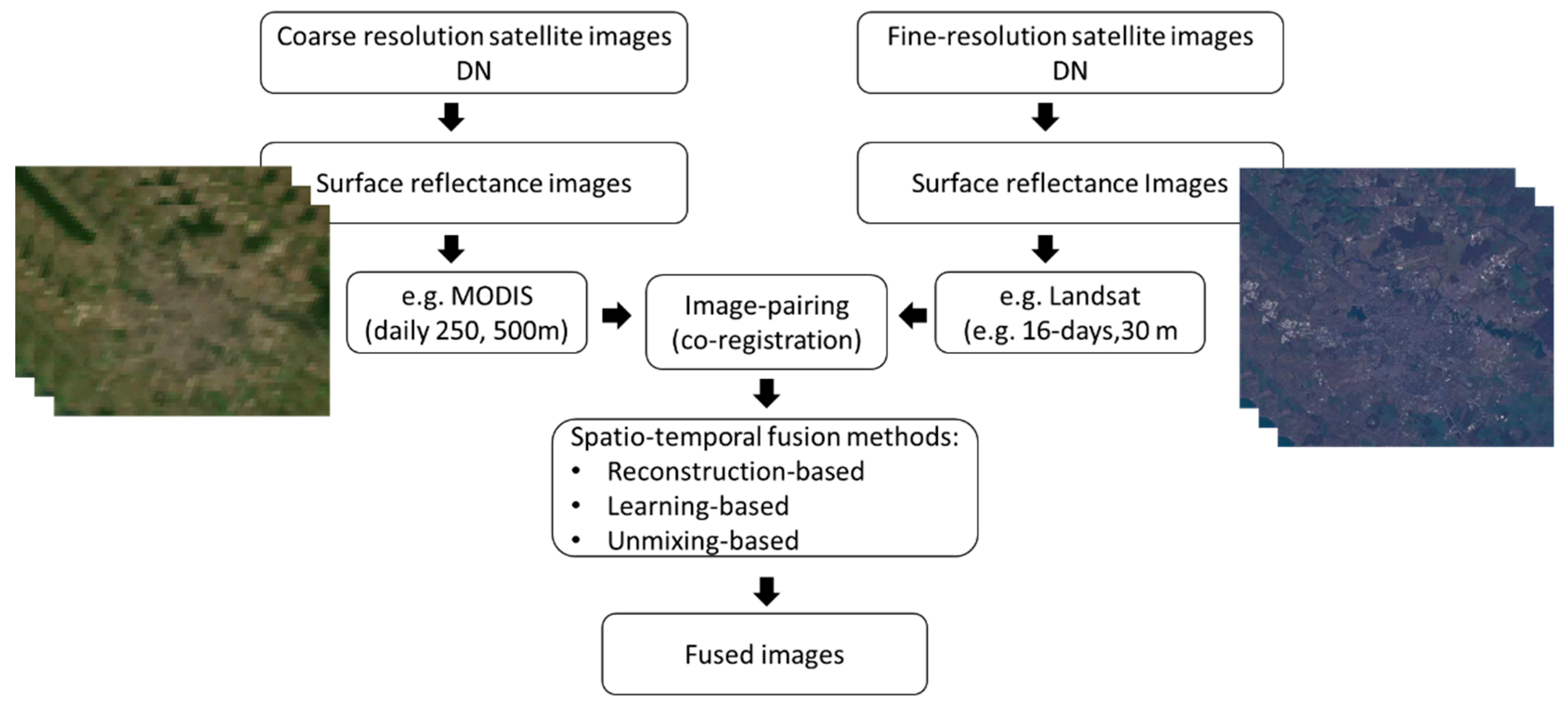
2. Fusion Methods to Increase Spatiotemporal Resolution of Satellite Images

Data fusion is a well-established research field [1,2,3,4]. Image fusion methods are primarily used for improving the level of interpretability of the input data [17]. Additionally, they can be utilized to address the problem of missing data caused by cloud or shadow contamination in satellite images time series [18,19,20]. According to Schmitt and Zhu [21] “the main objective of data fusion is either to estimate the state of a target or object from multiple sensors, if it is not possible to carry out the estimate from one sensor or data type alone, or to improve the estimate of this target state by the exploitation of redundant and complementary information”. The authors included in their study 12 definitions of data fusion from different application domains including computer science, information theory, tracking or surveillance [21].

Image fusion can be performed at pixel-level, feature-level (e.g., land-cover classes of interest), and decision-level (e.g., purpose driven) [5,11] by considering the following image blending scenarios: (1) combining high and low-spatial resolution images from the same satellite system, e.g., 15 m panchromatic images with 30 multispectral images from Landsat satellite, or from different satellite systems, e.g., SPOT 10 m panchromatic with Landsat multispectral images at 30 m spatial resolution [22]; (2) combining optical and microwave remote sensing images [17,23,24,25,26,27,28,29]; (3) combining multispectral satellite imagery and Light Detection and Ranging (LiDAR) data [30]; (4) combining multispectral satellite imagery and hyperspectral data [31], (5) combining high-resolution, low-frequency images with low resolution, high-frequency images [32] and (6) fusing microwave (passive) and microwave (active) sensors [33].

Long revisit time is not suitable for seasonal vegetation phenology monitoring or rapid surface changes. Therefore, we need high-resolution images in both time and space. Commercial satellites offer images at fine spatial scale and high temporal resolution. Among these sensors, we can mention the micro-satellites launched by Planet Labs [34] which acquire daily images of the Earth with a spatial resolution of about 3 m, or RapidEye sensors which acquire images with 5 m spatial resolution every day. Yet, these images are too costly for many applications in areas as diverse as agriculture mapping, timely monitoring of natural hazards or mining and illegal deforestation activities monitoring [34,35]. During last years, there have been different free sensors acquiring images at an increased spatial (e.g., Sentinel-2) and temporal resolution (Sentinel-3). These images could serve as a solution to the above-mentioned challenge. In addition, spatiotemporal image fusion methods, called also spatiotemporal downscaling methods [36], represent an efficient solution to generate images at a high temporal resolution [37] for more detailed land cover mapping and monitoring applications [38] and to improve the resolution of historical satellite images.

Since its launch in the early 1970s, and especially after allowing the public access to the enormous data archives [39], Landsat data products have been used in different climate, biodiversity, water or agriculture mapping studies. These data products have a great potential to accurately map land cover classes and to monitor land surface parameters. However, these data have a revisit time of only 16 days and therefore, their potential use for monitoring gradual changes such as changes in vegetation phenology or soils moisture, just to give a few examples, is rather reduced, especially in cloudy areas (e.g., tropical areas), where only a few cloud-free images per year are available. NASA’s MODIS sensor, on the other hand, acquires data twice a day which makes them more suitable for various surface dynamics mapping. Therefore, to increase the temporal resolution of fine spatial resolution images, many spatiotemporal image fusion methods have been developed during the last years. These methods use spatial information from the fine spatial resolution images and temporal information from coarse resolution satellites images to generate high spatial-temporal images. Spatiotemporal image fusion methods apply several steps to generate high spatiotemporal images: (1) both coarse and fine-resolution satellite images Digital Numbers (DN) have to be atmospherically corrected; (2) the pair-images have to be geometrically corrected and (3), in the end, one of the existing spatiotemporal fusion methods is applied to generate images which are at an increased spatial and temporal resolution (Figure 1). When the application required, calculation of indices before spatiotemporal fusion is performed [40].

According to Chen et al. [41], spatiotemporal image fusion methods can be classified into three categories: (1) reconstruction-based; (2) unmixing based and (3) learning-based methods. The advantages and disadvantages of these methods are presented in [42]. An overview of some of the existing spatiotemporal image fusion methods are presented in

Table 1. Overview of some of the spatiotemporal image fusion methods developed for blending high spatial resolution images with high temporal resolution images. The dark-grey highlighted methods are those based on feature fusion level, whereas the remaining ones are based on pixel fusion level.

	Spatiotemporal Fusion Model	Categories
Gao et al. [32]	Spatial and Temporal Adaptive Reflectance Fusion Model (STARFM)	Reconstruction-based
Hilker et al. [43]	Spatial-Temporal Adaptive Algorithm for mapping Reflectance Change (STAARCH)	Reconstruction-based
Zhu et al. [44]	Enhanced spatial and temporal adaptive reflectance fusion model (ESTARFM)	Reconstruction-based
Hazaymeh and Hassan [45]	Spatiotemporal image-fusion model (STI-FM)	Reconstruction-based
Luo et al. [46]	Satellite Data Integration (STAIR)	Reconstruction-based
Zhao et al. [47]	Robust Adaptive Spatial and Temporal Fusion Model (RASTFM)	Reconstruction-based
Wang and Atkinson [48]	FIT-FC	Reconstruction-based
Chen et al. [41]	Hierarchical Spatiotemporal Adaptive Fusion model (HSTAFM)	Learning-based
Huang et al. [7]	Sparse representation based Spatio temporal reflectance Fusion Model (SPSTFM)	Learning-based model
Song and Huang [49]	One-pair learning image fusion model	Learning-based model
Wu et al. [50]	Spatial and Temporal Data Fusion Approach (STDFA)	Unmixing-based
Huang and Zhang [51]	Spatio-Temporal Reflectance Fusion Model (U-STFM)	Unmixing-based
Gevaert et al. [36]	Spatial and Temporal Reflectance Unmixing Model (STRUM)	Unmixing-based
Wu et al. [52]	Modified Spatial and Temporal Data Fusion Approach (MSTDFA)	Unmixing-based
Zurita-Milla et al. [53]	Constrained unmixing image fusion model	Unmixing-based
Zhang et al. [54]	Spatial-Temporal Fraction Map Fusion (STFMF)	Unmixing-based
Zhu et al. [12]	Flexible Spatiotemporal Data Fusion (FSDAF)	Hybrid

. These methods have been successfully applied in different application domains including forest and crop monitoring, daily-field scale evapotranspiration etc. [10].

We evaluated how many times the above-listed methods were evaluated using the Web of Science database (Figure 2). This evaluation revealed that STARFM method, followed by ESTARFM and STAARCH are among the most popular spatiotemporal image fusion methods.

2.1. Reconstruction-Based Spatiotemporal Image Fusion Methods

Reconstruction-based spatiotemporal methods are also called filter-based methods [55] or weighted-function-based [56] and are used to generate synthetic spectral reflectance by means of the weighted sum of the neighboring similar pixels of the input image source. A widely-used reconstruction-based image fusion methods is the STARFM [32]. This method generates synthetic high-resolution images (e.g., 30 m resolution) on a daily basis by employing a neighborhood weighting process. It assumes the existence of co-temporal pairs of fine spatial resolution and coarse spatial resolution images and, therefore, the quality of the fused time series is dependent on the number of observations from the high temporal resolution images set [57] and on the availability of cloud-free pair images of the matching dates [46]. When no-matching dates images are found, the method starts searching for the closest image in the temporal domain to predict the value in the fine resolution output image. STARFM involves four main steps. First, coarse resolution images are co-registered and resampled to the resolution of the high spatial resolution images, e.g., 30 m for Landsat 8. In the next step, a moving window (w) is applied to identify similar pixels in the fine resolution images. In the third step, a weight is assigned to the homogeneous pixels based on the following criteria: (1) the spectral difference between the surface reflectance of the images pair; (2) the temporal differences in the dates of the coarse resolution, high frequency images (date of the pair-images and the prediction date); (3) the Euclidean distance between the neighbor and the central pixel. In the last step, the surface reflectance of the central pixel is calculated based on the following equation:

$$\begin{array}{cc}\hfill FR(\frac{w}{2},\frac{w}{2}{t}_{pr})=& {\displaystyle {\displaystyle \sum }_{i=1}^N}{W}_{ik}\ast (FR(x_i,y_i,t_0)+(CR\left(x_i,y_i,t_{pr}\right)\hfill \\ & -CR\left(x_i,y_i,t_0\right)\hfill \end{array}$$

(1)

where $FR\left(\frac{w}{2},\frac{w}{2}{t}_{pr}\right)$ represents the central pixel of the moving window (w) to be predicted for the fine resolution images at time $t_{pr}$, P is the total number of pixels in FR and CR images, N is the total number of pixels within the defined moving window, $CR\left(x_i,y_i,t_{pr}\right)$ represents the pixels values of the coarse resolution data on the prediction date, $FR\left(x_i,y_i,t_0\right)andCR\left(x_i,y_i,t_0\right)$ represent the pixel values of the base pair input images and $W_{ik}$ represents the weight assigned to the similar neighboring pixels.

Zhu et al. [44] proposed the extension of the STARFM method [32] and developed an enhanced spatial and temporal adaptive reflectance fusion method which proved to successfully predict fine resolution reflectance, especially in complex and heterogeneous landscape. The method requires two or more pairs of fine-coarse resolution images collected on the same day and a series of time series coarse resolution data for prediction dates. Emelyanova et al. [58] found out that this new method performed better than the method proposed by Gao et al. [32] in areas with spatial variance dominance, but is less successful in areas where the temporal variance was dominant.

These methods were successfully tested for fusing Landsat-MODIS images [36]. A more generic spatiotemporal image fusion method, in terms of the used input images, was developed by Luo et al. [46]. The method firstly applies a data gap-filling procedure, followed by an interpolation model for capturing the spatial information available in the image with the highest spatial resolution. The relationship between the fine resolution and coarse pixels is modeled using the following formula:

$$\begin{array}{cc}\hfill FR\left(x,y,t_i\right)& =CR\left(x,y,T_j\right)\hfill \\ & +\epsilon \left(x,y,t_i\right)\hfill \end{array}$$

(2)

where x, y represents the aligned fine resolution (FR) and coarse resolution (CR) pixels, $T_j$ is the acquisition date for the pair-images and $\epsilon \left(x,y,t_i\right)$ represents the differences between the pixels of the two images (i.e., errors) caused by e.g., viewing angle geometry. The prediction of the fine resolution pixels values (FR) at $t_{pr}$ is performed as follows:

$$\begin{array}{cc}\hfill FR\left(x,p,t_{pr}\right)& =CR\left(x,y,t_p\right)\hfill \\ & +\mathsf{\Delta }\left(x,y,t_p\right)\hfill \end{array}$$

(3)

where $\mathsf{\Delta }\left(x,y,t_p\right)$ represents the difference between the spectral reflectance values of the two input pair images at location x, y and date $t_{pr}$.

Two types of temporal changes need to be considered when developing spatiotemporal fusion methods, namely the seasonal change of vegetation, i.e., vegetation phenology, and the land cover change, i.e., deforestation. While the first temporal change is successfully considered by the method proposed by Gao et al. [32] and by Luo et al. [46], the second temporal change required further developments.

Hilker et al. [43] proposed a spatial temporal adaptive method for detecting reflectance changes associated with land cover change and disturbance. This image fusion method uses high spatial resolution tasseled cap transformation and high frequency of tasseled cap transformation to identify changes in reflectance. The developed method is simple and intuitive and requires at least two fine resolution images representing the beginning and the end of the user-defined time interval. These two images are used to identify the changes in the data. The changes are calculated using the so-called Disturbance Index (DI) which relies on three tasseled cap indices, namely brightness, greenness, and wetness.

This index identifies the changes (or disturbances) in the coarse resolution pixel values between two consecutive dates. The presence of a disturbance event in the study area influences which pair images are used for predicting the reflectance value of the fine resolution images. For example, if the disturbance occurs after the prediction date, then the first fine-course resolution pair-images is used. If the pixel to be predicted lies after the occurrence of the disturbance, then the last pair-images is used. While this method is one of the initial image fusion efforts which consider landscape changes [7], there are studies which reported that it is suited only for forest disturbances scenario as the method selects the optimal fine resolution image date for prediction based on forest disturbance date detection from coarse resolution images. Therefore, this method is of limited value if when other types of land cover changes occur in the investigated areas.

Zhao et al. [47] developed a method called robust adaptive spatial and temporal fusion method, which is capable to consider not only gradual changes, i.e., shape change (e.g., crop rotation), but also abrupt changes such as urban sprawl. To do this, the authors extended the spatiotemporal image fusion method of Gao et al. [32] by replacing the Inverse Distance Weighted (IDW) with a local linear regression model to calculate the weights assigned to the pixels similar to the central pixel. To do this, the method (which uses only one prior pair of fine-coarse resolution images) follows three steps. First, it searches for similar neighboring pixels in the searching moving window as:

$$\begin{array}{c}w\left(c,s\right)\\ =\frac{1}{Z\left(c\right)}{e}^{-||P_{\left(c,t0\right)}-P_{\left(s,t0\right)}||2a^2}\end{array}$$

(4)

where c represents the central pixel, s represents the similar pixels, $||P_{\left(c,t0\right)}-P_{\left(s,t0\right)}||2a^2$ is a Gaussian kernel and Z(c) is a normalizing constant:

$$Z_c={{\displaystyle \sum }}_i{e}^{-||P_{\left(c,t0\right)}-P_{\left(s,t0\right)}||2a^2}$$

(5)

Second, it calculates the similar neighbor’s weights based on the spectral differences between the pixels in the fine resolution and coarse resolution images, the temporal differences between the input and prediction dates of the fine resolution images and the spectral difference between the central pixels and neighboring pixels.

The third step consists of predicting the spectral reflectance of the fine resolution pixels (FR) as:

$$\begin{array}{c}F{R}_{\left(c,tpr\right)}={{\displaystyle \sum }}_{s=1}^n{W}_s\ast (p_{\left(s,t_{pr}\right)}-p_{\left(s,t_0\right)}+P_{(s,t_0)})\end{array}$$

(6)

where $p_{\left(s,t_k\right)}$ and $p_{\left(s,t_0\right)}$ represent the coarse resolution images pixels that spatially correspond to high resolution pixels $F{R}_{(s,t_0)}$.

As presented above, these methods are very efficient for spatiotemporal image fusion in relatively homogeneous landscape and when the input images have the same input spectral values. Nevertheless, there is a need for spatiotemporal fusion methods capable to use different images as input, i.e., images with different spectral values (such as learning-based methods) and methods capable to be applied in a heterogeneous landscape where pixels from the coarser satellite images are mixed (such as unmixing-based methods).

2.2. Learning-Based Spatiotemporal Image Fusion Methods

Learning-based methods use machine learning to predict finer temporal resolution images from coarse spatial resolution images [56]. Compared to reconstruction-based and unmixing-based methods which allows spatiotemporal fusion of images with unified spectral values, learning-based methods allows fusion between images with different spectral values. One of the first studies dedicated to using sparse representation method into data fusion is presented by Huang et al. [7]. Sparse representation methods learn the differences between fine spatial resolution images and high temporal coverage images [59] by making use of a dictionary created from the image patches generated from the two image types. Similar to reconstruction-based methods, important research efforts were dedicated to developing a learning-based method that considers the phenology of vegetation and other disturbances caused by land cover changes that might occur before the prediction date. In this context, Huang et al. [7] developed an image fusion method which accounts for both vegetation phenology and land cover changes occurring over the observation period of the fused images. The original implementation of the method relies on fine-coarse resolution image pairs before and after prediction date, and one coarse resolution image at prediction date. Later, the authors extended their method to consider one fine-coarse resolution image-pairs instead of prior and posterior pairs of images. The new spatiotemporal image fusion method is called SP-One [49].

Chen et al. [41] proposed a hierarchical spatiotemporal adaptive fusion method capable of predicting temporal changes such as seasonal phenology and land-cover changes using only one image pair (one prior or posterior image pair). The authors compared the results obtained by this method with those obtained by the spatiotemporal image fusion methods proposed by [12,32,49] and concluded that their method performed better especially in capturing land cover changes in the predicted fine resolution reflectance images. Kwan et al. [60] proposed a spatiotemporal image fusion method which relies on learning the mapping between MODIS images (or between overlapping or non-overlapping patches from the two images obtained by k-means classifier) and is applied to an earlier acquired Landsat image to predict an image at a later time. The method can be easily adapted to new multisource images. However, it performed worse than other spatiotemporal image fusion methods when applied in a heterogeneous landscape, where the pixels from the coarser satellite images are not pure. Therefore, a new category of spatiotemporal image fusion methods can be used to address this challenge, namely those based on spectral unmixing models [61].

2.3. Unmixing-Based Spatiotemporal Image Fusion Methods

The need to fuse images from very heterogeneous environments has been systematically addressed by the unmixing-based spatiotemporal image fusion methods. Spectral unmixing methods rely on the linear spectral mixture to extract endmembers and abundances, i.e., proportion, at the sub-pixel level [36]. The number of endmembers and abundances is obtained from a high-resolution data set, and the spectral signature of the endmembers is unmixed from the coarse resolution images. Linear mixed methods assume that “the reflectance of each coarse spatial resolution pixel is a linear combination of the responses of each land cover class contributing to the mixture” [52]. Thus, spectral reflectance of coarse resolution pixels $CR\left(i,t_i\right)$ consisting of n land cover classes is weighted by classes abundance as follows [52]:

$$CR\left(i,t_i\right)={\displaystyle \sum }_{c=0}^n{f}_c\left(i,c\right)\times {\overline{r}}_f\left(c,t_i\right)+\epsilon \left(i,t_i\right)$$

(7)

where fc(i,c) is the abundance of land cover class c in coarse pixel i; $\overline{r}$_f(c,t_i) is the mean reflectance of pixels from the fine resolution images belonging to land cover class c at time t_i; and $\epsilon$(i,t_i) is the residual.

Unmixing-based methods usually start with the classification of the image with high spatial resolution using unsupervised methods such as k-means (or fuzzy k-means), followed by the spectral unmixing of the image with high temporal frequency by making use of the classification information obtained during the first step [36,61]. Alternatively, up-to-date land cover/land use maps can be used to identify the endmembers as shown by Zurita-Milla et al. [53]. A comparison between unmixing-based image fusion and reconstruction-based methods is provided by Gevaert et al. [36]. The authors also implemented a Bayesian unmixing-based fusion method to downscale coarse resolution images to the spatial resolution of fine resolution images using one base fine-coarse resolution image pair. This method outperformed those proposed by [32] when fewer input fine resolution images area used.

Given the landscape heterogeneity and complexity caused by different geomorphological conditions or anthropogenic activities, land cover change is expected during the period of blended images [62]. To address this problem, [50] proposed a spatiotemporal image fusion method based on unmixing and using two or more image pairs. The authors assumed that the spectral information of pixels belonging to the same class have the same temporal variation. This method has been successfully used for high-resolution (i.e., 30 m) leaf area index estimation [63], for generating daily synthetic Landsat imagery [52] or for land surface temperature [64]. Since it neglects the differences among different sensors and thus the window size is fixed, Wu et al. [52] introduced a modified spatial and temporal data fusion method by including adaptive window size and moving steps selection for disaggregating coarse pixels. The method requires fine resolution images acquired at the beginning and end of the observation period, coarse resolution reflectance data acquired on the same date as fine resolution data and land cover data to predict daily fine resolution images.

Huang et al. [51] described an image fusion method capable to account for both phenological and land-cover changes. The method requires two pairs of fine-coarse resolution images at the beginning and end of the observation period and a coarse resolution image for the prediction date. Proposed data fusion is sensitive to the scale parameter used to delineate homogeneous change regions from fine resolution images through segmentation. It proved, however, to perform better than reconstruction-based [32] and other spectral unmixing based methods [44], mainly because it relies on neighboring spatial information for blending the images, whereas the other evaluated methods consider linear land cover change during the observation period. Additional unmixing-based methods dedicated to fusing Landsat and Medium Resolution Imaging Spectrometer (MERIS) are described by [53,65]. Zurita-Milla et al. [53] described a linear mixing method to downscale MERIS data from 300 m to 25 m resolution using the Dutch land use database to derive the fractional composition of input pixels.

Besides the above presented methods, we also have the so called hybrid methods that rely on different technologies to perform the fusion. Zhu et al. [12], for example, developed a spatiotemporal image fusion method capable to predicting pixel values at fine resolution in challenging situation such as heterogeneous areas and where land cover change occurs during the period between the input and prediction dates. First, this method assumes that all pixels of coarse resolution images are mixed pixels. The reflectance of these pixels can be described using a linear mixture model:

$$C_m={\displaystyle \sum }_{i=1}^M{f}_i\left(\frac{1}{a}{F}_{im}-\frac{a}{b}\right)+\epsilon$$

(8)

$$C_n={\displaystyle \sum }_{i=1}^M{f}_i\left(\frac{1}{a}{F}_{in}-\frac{a}{b}\right)+\epsilon$$

(9)

where $C_m$ and $C_n$ represent the reflectance of the mixing pixel at date $t_m$ and $t_n$, $f_i$ is the fraction of the i-th land cover, $F_{im}$ and $F_{in}$ represent the reflectance of the i-th land cover at date, and $t_m$, $t_n$, a and b represent the coefficients of the linear regression model developed for relative calibration between fine resolution and coarse resolution images.

Second, the changes of coarse-resolution reflectance from $t_m$ and $t_n$ is calculated as follows:

$$C_n-C_m={\displaystyle \sum }_{i=1}^M\frac{f_i}{a}\left(F_{in}-F_{im}\right)$$

(10)

Similar to Zhu et al. [12], Zhang et al. [54] developed a method for fusing coarse-spatial, fine-temporal and fine-spatial, coarse-temporal images that assumes that surface reflectance values of coarse resolution pixels are mixed. The method relies on predicting the fraction map of fine resolution images from the available coarse resolution fraction maps by making use of images acquired before and after the prediction dates. The fraction maps can be obtained using any available spectral unmixing model such as a linear spectral mixture model or multiple endmember spectral mixture analysis model.

3. Synthesis: Challenges and Opportunities

The spatiotemporal image fusion methods reviewed in this paper generate images at a higher temporal resolution which can be further used for land surface monitoring applications, especially in cloudy areas (e.g., tropical areas), where only a few cloud-free images per year are available. Leckie [66] reported, for example, that there is a 10% probability of acquiring cloud-free images such as Landsat for a certain time interval. The problem of data gaps caused by the presence of clouds can be addressed by combining microwave images with optical images similar to the approach proposed by Mizuochi et al. [27], who proposed fusing Advanced Microwave Scanning Radiometer (AMSR) series with MODIS images followed by MODIS-Landsat fusion.

Developed spatiotemporal image fusion methods have been successfully used to fuse optical images collected by different remote sensing platforms. Wu et al. [67] reconstructed daily 30 m remote sensing data from Huanjing satellite constellation, Gaofen satellite, Landsat, and MODIS data using the spatiotemporal methods developed by Wu et al. [50]. Generated remote sensing data are efficient for extracting vegetation phenology and for mapping crops with an overall accuracy higher than those obtained from multi-temporal Landsat NDVI data. Quan et al. [68] proposed a method to fuse Landsat, MODIS and geostationary satellites to 100 m resolution and one-hour interval. This method was compared with those developed by Gao et al. [32], Zhu et al. [44], and Wu et al. [69] and proved to perform better over heterogeneous landscapes and changing land cover types. Kwan et al. [70] evaluated how existing spatiotemporal image fusion methods perform for fusing Planet and WorldView images scenarios, and emphasized the importance of reducing the magnitude differences in the reflectance values between the two input sensors products and of aligning them to avoid misregistration errors. Wang et al. [71] fused MSI and OLI sensors for a study dedicated to land cover/land use mapping and proved that land cover change accuracy increases when Landsat-8 panchromatic band is used in the image fusion task. This is one of the few studies which fuses the two sensors products.

3.1. Other Advanced Methods for Spatiotemporal Image Fusion

Deep learning has gained the attention of the remote sensing community in the last years for various image understanding and image classification problems [72]. It has for example been successfully used for pan-sharpening [73,74,75,76], feature and decision-level fusion [77,78] and spatial-spectral image fusion [79,80,81]. An overview of deep learning for data fusion is provided by Liu et al. [82] and Audebert et al. [30]. Despite its proven efficiency in different image fusion scenarios, this method has rarely been used for spatiotemporal image fusion. Song et al. [83] proposed a CNN model for fusing Landsat and MODIS data by considering both spatial heterogeneity of the landscape and temporal changes occurring during the observation period. Our remote sensing community could further benefit from advances in deep learning occurring in computer vision where efficient convolutional networks for learning spatiotemporal features from video dataset have been successfully developed [84].

Bayesian methods have been successfully applied for fusing images in the spatial and spectral domain [85]. Despite their ability to handle uncertainties in input images, a rather reduced number of Bayesian methods for spatiotemporal fusion of satellite images have been developed [86,87].

Another example of spatiotemporal image fusion methods includes those based on physical models. Roy et al. [88], for example, proposed a semi-physical fusion method that uses MODIS Bi-directional Reflectance Distribution Function (BRDF)/Albedo to predict BRDF at the spatial resolution of the ETM+ images.

3.2. Increasing the Resolution of Various Satellite-Derived Data Products

Important research efforts are dedicated to increasing the resolution of satellite-derived products such as NDVI, land surface temperature, evapotranspiration, and precipitation. In order to obtain a better resolution of these data products, several studies used the remote sensing data whose spatiotemporal resolution has been improved by means of one of the methods presented in this paper.

A large number of these studies are dedicated to land surface temperature data, mainly because these data are important in a wide range of environmental modeling applications from local to global scales [89,90]. There are basically two main methods used to increase the coarse resolution of land surface temperature, namely the methods which rely on physical models and those using statistical models [15] such as the linear regression models [91,92], co-kriging model [93] or random forest (RF) regression [89,94]. Yang et al. [94] used a random forest model to downscale MODIS based land surface temperature in arid regions from 1 km to 500 m. Yang et al. [95] proposed a disaggregation method for subpixel temperature using the remote sensing endmember index-based method. ASTER visible and near-infrared bands and shortwave bands at 30 m spatial resolution were used in combination with the 990 m resolution MODIS land surface temperature data. Merlin et al. [96] disaggregated MODIS surface temperature at 100 m by considering the temperature difference between photosynthetically and non-photosynthetically active vegetation. For this study, the authors used Formosat-2 data due to their high spatial resolution, i.e., 8 m, and high temporal resolution, i.e., one image per day. Wu et al. [64] applied the spatiotemporal data fusion methods developed by [32,44,50] to generate high temporal and high spatial resolution land surface temperature product by combining ASTER and MODIS data products. The authors concluded that the quality of the generated land surface temperature products increased by using high spatiotemporal resolution satellite images.

A region-based and pixel-based disaggregation method is proposed by Alidoost et al. [97] to improve the resolution of evapotranspiration data from MODIS images from 1 km to 250 m and further to 30 m resolution. Liu et al. [98] proposed the extension of the traditional cokriging method from the spatial domain to spatiotemporal domain capable to account for spatiotemporal structures of the input images. The method was tested for fusing MODIS NDVI images available at 250 m with ETM+ 30 m NDVI images. Hwang et al. [99] fused multi-temporal MODIS and Landsat data together with topographic information for a better estimation of biophysical parameters over complex terrain. Data were validated by making use of a ground-based continuous fraction of absorbed photosynthetically active radiation and leaf area index measurements.

Several studies were dedicated to increasing the spatial resolution of soil moisture through disaggregation methods [100,101]. Jia et al. [102] disaggregated tropical Rainfall Measuring Mission dataset using digital elevation model data and SPOT satellite images The results were validated by using in-situ data from different local stations present in the study area, i.e., Qaidam basin. Duan and Bastiaanssen [103] disaggregated the same data product on the basis on a rather limited number of rain gauge data sets. The authors generated an improved monthly pixel-based precipitation with a special resolution of 1 km.

3.3. Methods to Increase Spatiotemporal-Spectral Resolution of Images

Most image fusion methods described in this paper are dedicated to increasing the spatiotemporal resolution of input images. Only a few methods enable the fusion of spatiotemporal and spectral information [55,104,105]. Huang et al. [104] described a Bayesian method to generate synthetic satellite images with high spectral, temporal and spectral resolution. Meng et al. [105] developed a unified framework for spatiotemporal-spectral fusion based on maximum posteriori theory. The framework was successfully tested on QuickBird, ETM+, MODIS, Hyperspectral Digital Imagery Collection Experiment (HYDICE) and SPOT-5 images [55].

3.4. Quality Assessment of Spatiotemporal Blended Images

Validation of the generated image fusion products is performed either visually, i.e., using a qualitative assessment [106] or by employing a quantitative metric [1,107]. Among these metrics we can refer to spectral angle mapper [108], peak signal-to-noise ratio [109], structural similarity index used to assess the spatial distortion of the fused image [12], image quality index proposed by [110] and its vector extension [111], absolute difference [60,112], root mean squared error (RMSE) [112], cross-correlation [112] and Erreur Relative Globale Adimensionnelle de Synthese [113]. The performance of the developed data fusion methods is evaluated by either using real data or synthetic data [32,51,60]. There are studies which evaluated the quality of the fused images by using evaluation metrics which do not require reference data [114,115]. The most used quantitative evaluation metrics available in the literature are presented in

Table 2. Most common metrics used to evaluate the accuracy of the spatiotemporal fused product.

Data Fusion Performance Metrics	Authors
Spectral angle mapper (SAM)	Yuhas et al. [108]
Peak Signal-to-noise-ratio (SNR)	Sheikh et al. [116]
Structural Similarity Index (SSIM)	Wang et al. [117]
Image quality index	Wang et al. [110]
Extended image quality index	Alparone et al. [111]
Quality w/no reference index	Alparone et al. [114]
Enhancement measure evaluation (EME)	Agaian et al. [115]
Entropy	Tsai et al. [118]
Erreur Relative Globale Adimensionnelle de Synthese (ERGAS)	Wald [113]

.

Currently, there is no agreement on which spatiotemporal image fusion method performs best for blending fine spatial resolution images with high temporal coverage images [42]. Wu et al. [64] compared the methods developed by [32,44,50] for generating high temporal and spatial resolution LST product from ASTER and MODIS LST data in different landscape areas and concluded that all methods perform satisfactorily especially in desert areas. Furthermore, the spatiotemporal data method developed by Wu et al. [50] is capable to deal with noises in the data much better than the other two evaluated methods. Chen et al. [42] compared several image fusion methods and concluded that those relying on reconstruction-based concepts and theories are more stable than the learning-based methods.

Kwan et al. [60] argued that none of the available image fusion methods perform well under all conditions of remote sensing applications. To test this hypothesis, we need a ready to use and open access library of the available image fusion methods [70] that would allow us to compare them across different landscapes [42] and agroecological regions, taking into account their sensitivity to noises in the data or to spatial and temporal variances [58]. Additionally, a hybrid image fusion framework can serve as a viable solution to combine methods that work well for heterogeneous landscape with those which perform well under homogeneous landscape conditions.

Uncertainty analysis of the predicted/fused spatiotemporal images has been neglected by many fusion methods presented in this paper. Recently, Wang and Huang [119] proposed a spatiotemporal fusion method based on the geostatistical ordinary kriging method that allows the estimation of the prediction uncertainty. The method proposed by Zhong and Zhou [120] enables not only the estimation of the uncertainty of the predicted image, but it accounts also for the uncertainties of the input images used for the fusion purpose.

3.5. Spatiotemporal Image Fusion Methods for Sentinel Images

The new program of the European Space Agency (ESA), namely the Sentinel missions, gained the attention of the remote sensing community due to the increasing spatial, spectral and temporal resolution [121]. In the perspective of combined use of Sentinel-2 and Landsat 8, there are several differences to be considered. For example, in a previous study [122] we found out relatively high discrepancies between Normalized Difference Vegetation Indeed (NDVI) computed from Sentinel-2 and Landsat-8. We concluded in that work that, in order to take advantage of the 10 m resolution of Sentinel-2 and use these data along with Landsat-8 data, it would be desirable to adjust the reflectance values of the two sensors. A useful method for this purpose could be the one presented by Flood [123] or co-registration techniques such as phase correlation [124]. Besides differences in spectral values, previous studies also reported a misalignment of several pixels between Landsat 8 and Sentinel-2 [125]. Therefore, images coming from the two sensors need to be co-registered before any concurrent use. Further information on Sentinel-2 MSI and Landsat-8 OLI sensors characteristics is provided by Zhang et al. [126].

Wang et al. [48] described an advanced method to fuse MSI onboard Sentinel-2 platform and OLCI onboard Sentinel-3 platform which relies on regression model fitting to relate spectral reflectance from two acquisition times and spatial filtering to remove the artifacts in the regression model fitting prediction. Their proposed method accounts successfully for the temporal land cover changes when creating nearly daily Sentinel-2 images. Furthermore, it relies on a single Sentinel-3/Sentinel 2 images pair. Besides these studies dedicated to Sentinel missions, important research has been dedicated to developing more generic methods which can be used to fuse different sensors products. An example of such a method is those developed by Luo et al. [46].

It is expected that a large number of spatiotemporal image fusion methods will be developed in the future in order to leverage the available satellite data archive and to increase the spatial resolution of the latest satellite images such as those acquired by microsatellites (e.g., planet images).

3.6. Important Data Pre-processing Issues to be Considered when Fusing Spatiotemporal Images

When developing new spatiotemporal image fusion methods, the following issues need to be considered [46,88]:

• Spectral responses of input images have to be unified: Reconstruction and unmixing spatiotemporal image fusion methods assume that input images have similar spectral information. Therefore, their application is limited, given that the sensors might have different wavelength. When blending information from different remote sensing data sources, we have to spectrally normalize the input sensors to common wavebands [70]. According to Pinty et al. [127], the absence of similar wavelength has a low impact on the fusion results when physically-based reflectance methods are used for blending surface reflectance of the input images. Machine learning based spatiotemporal image fusion methods, on the other hand, are less sensitive to similarity between spectral responses of the input images.
• Co-registration of multi-source input images: Multi-source images alignment is a very important issue to be considered when fusing them. For example, reported misalignments between Landsat and Sentinel-2 by several pixels need to be carefully addressed when fusing the two input images [125]. Further investigation in the development of automatic solutions for images alignments is highly required [70].
• Atmospheric corrections: Radiometric consistency of the multi-source images to be fused might vary because of the presence of clouds and haze, or because of the differences in the illumination and acquisition angles [88]. Therefore, input images have to be radiometrically corrected before fusing them [70] using one of the available existing radiometric corrections techniques such as MODerate spectral resolution TRANsmittance code (MODTRAN) [128]. These techniques can be grouped into two categories, namely absolute and relative techniques. Absolute techniques require information on the sensor spectral profile for sensor calibration and corrections of images for atmospheric effects [129]. Relative radiometric techniques involve either the selection of landscape elements whose reflectance remain constant over time [130,131] or normalization using regression [132,133].

3.7. Future Directions

Image fusion methods need to be flexible enough to accomplish different fusion tasks under different environmental conditions [55,104,105]. While most of the presented spatiotemporal image fusion methods are capable enough to capture reflectance changes which are caused by vegetation dynamics through time, i.e., vegetation phenology, not all of them account for sudden land cover changes (e.g., deforestation, flooding events) that might occur during investigated observational time [47]. More efforts are, therefore, required to capture accurate temporal changes when fusing high spatial resolution and high frequent temporal coverage from different remotely sensed data [43,51]. By considering temporal changes, spatiotemporal fusion methods can be successfully used for mapping and monitoring applications in areas with rapid land cover changes [41,55].

Given the increasing number of new sensors which acquire images at fine spatial and spectral resolution, we consider that spatiotemporal image fusion methods should be extended to fuse multi-sensor images, i.e., more than two sensor types data over a specific observation period. Indeed, this is a challenging task given the diversity of images to be fused in terms of spectral, spatial, temporal and radiometric resolution. In this context, Dynamic Time Warping could offer a flexible framework for performing spatiotemporal fusion of different images accurately. This is due to the ability of this method to predict the surface reflectance pixel values by accounting for the phenological changes of vegetation and by the presence of clouds which contaminate the pixels values.

Another important issue to be considered in the future is the computational time. As an increasing amount of data to be fused is available, the fusion methods have to be capable to scale up to regional and global scales [46]. They can be included into operational applications for various image fusion tasks by making use of advanced cloud computing technologies such as Google Earth Engine [134]. This will allow almost near-real time fusion of images, a task that is of paramount importance for disaster management activities.

4. Conclusions

Three categories of spatiotemporal image fusion methods have been discussed in this paper, namely reconstruction-based, learning-based and unmixing based methods. The most popular method for blending fine-spatial resolution with high-temporal resolution images is the reconstruction-based STARFM. Recently, new methods have been developed to fuse images acquired by other sensor products, e.g., Sentinel-2, Sentinel-3 or images acquired by microsatellites. Also, many reviewed methods account for land cover changes occurring during the observation period. The problem of cloud obscuration can be solved by fusing microwave data with optical images.

Future efforts are required for generating spatiotemporal image fusion solutions which are: (1) generic enough to consider various sensors characteristics; (2) computationally efficient to be able to scale up to regional and global level; (3) robust to temporal and spatial variations specific to landscape of a different heterogeneity and complexity caused by different physio-geographical conditions, soil or land management practices, (4) flexible enough to consider phenological dynamics of vegetation or land cover changes caused by both external factors, such as natural hazards and anthropogenic activities, i.e., urban sprawl, and (5) testing and implementation of more sophisticated machine learning methods such as deep learning. It is unlikely that there will be a single optimal spatiotemporal method capable to address data blending needs of various remote sensing applications [70]. Therefore, an efficient and operational framework for benchmarking existing spatiotemporal image fusion methods similar to those developed by IEEE GRSS Data Fusion Contest is of paramount importance to help remote sensing community assess the performance of the spatiotemporal image fusion methods and the quality of the resulting output images.

References

1. Pohl, C.; Van Genderen, J. Remote sensing image fusion: An update in the context of digital earth. Int. J. Digit. Earth 2014, 7, 158–172. [Google Scholar] [CrossRef]
2. Ehlers, M.; Klonus, S.; Johan Åstrand, P.; Rosso, P. Multi-sensor image fusion for pansharpening in remote sensing. Int. J. Image Data Fusion 2010, 1, 25–45. [Google Scholar] [CrossRef]
3. Zhang, J. Multi-source remote sensing data fusion: Status and trends. Int. J. Image Data Fusion 2010, 1, 5–24. [Google Scholar] [CrossRef]
4. Wu, W.; Yang, J.; Kang, T. Study of remote sensing image fusion and its application in image classification. Int. Arch. Photogramm. Remote Sens. Spat. Inf. Sci. 2008, 37, 1141–1146. [Google Scholar]
5. PohlC, V.G.J.L. Multisensor image fusion in remote sensing: Concepts, methods and applications. Int. J. Remote Sens. 1998, 19, 823–854. [Google Scholar] [CrossRef]
6. Van Genderen, J.; Pohl, C. Image fusion: Issues, techniques and applications. In Proceedings of the EARSeL Workshop on Intelligent Image Fusion, Strasbourg, France, 11 September 1994; pp. 18–26. [Google Scholar]
7. Huang, B.; Song, H. Spatiotemporal reflectance fusion via sparse representation. IEEE Trans. Geosci. Remote Sens. 2012, 50, 3707–3716. [Google Scholar] [CrossRef]
8. Roy, D.P.; Wulder, M.; Loveland, T.R.; Woodcock, C.; Allen, R.; Anderson, M.; Helder, D.; Irons, J.; Johnson, D.; Kennedy, R. Landsat-8: Science and product vision for terrestrial global change research. Remote Sens. Environ. 2014, 145, 154–172. [Google Scholar] [CrossRef]
9. Mizuochi, H.; Hiyama, T.; Ohta, T.; Nasahara, K. Evaluation of the surface water distribution in north-central namibia based on modis and amsr series. Remote Sens. 2014, 6, 7660–7682. [Google Scholar] [CrossRef]
10. Gao, F.; Hilker, T.; Zhu, X.; Anderson, M.; Masek, J.; Wang, P.; Yang, Y. Fusing landsat and modis data for vegetation monitoring. IEEE Geosci. Remote Sens. Mag. 2015, 3, 47–60. [Google Scholar] [CrossRef]
11. Ghassemian, H. A review of remote sensing image fusion methods. Inf. Fusion 2016, 32, 75–89. [Google Scholar] [CrossRef]
12. Zhu, X.; Helmer, E.H.; Gao, F.; Liu, D.; Chen, J.; Lefsky, M.A. A flexible spatiotemporal method for fusing satellite images with different resolutions. Remote Sens. Environ. 2016, 172, 165–177. [Google Scholar] [CrossRef]
13. Atkinson, P.M. Downscaling in remote sensing. Int. J. Appl. Earth Obs. Geoinf. 2013, 22, 106–114. [Google Scholar] [CrossRef]
14. Thomas, C.; Ranchin, T.; Wald, L.; Chanussot, J. Synthesis of multispectral images to high spatial resolution: A critical review of fusion methods based on remote sensing physics. IEEE Trans. Geosci. Remote Sens. 2008, 46, 1301–1312. [Google Scholar] [CrossRef]
15. Zhan, W.; Chen, Y.; Zhou, J.; Wang, J.; Liu, W.; Voogt, J.; Zhu, X.; Quan, J.; Li, J. Disaggregation of remotely sensed land surface temperature: Literature survey, taxonomy, issues, and caveats. Remote Sens. Environ. 2013, 131, 119–139. [Google Scholar] [CrossRef]
16. Zhu, X.; Cai, F.; Tian, J.; Williams, T. Spatiotemporal fusion of multisource remote sensing data: Literature survey, taxonomy, principles, applications, and future directions. Remote Sens. 2018, 10, 527. [Google Scholar]
17. Reiche, J.; Verbesselt, J.; Hoekman, D.; Herold, M. Fusing landsat and sar time series to detect deforestation in the tropics. Remote Sens. Environ. 2015, 156, 276–293. [Google Scholar] [CrossRef]
18. Racault, M.-F.; Sathyendranath, S.; Platt, T. Impact of missing data on the estimation of ecological indicators from satellite ocean-colour time-series. Remote Sens. Environ. 2014, 152, 15–28. [Google Scholar] [CrossRef]
19. Honaker, J.; King, G. What to do about missing values in time-series cross-section data. Am. J. Political Sci. 2010, 54, 561–581. [Google Scholar] [CrossRef]
20. Dunsmuir, W.; Robinson, P. Estimation of time series models in the presence of missing data. J. Am. Stat. Assoc. 1981, 76, 560–568. [Google Scholar] [CrossRef]
21. Schmitt, M.; Zhu, X.X. Data fusion and remote sensing: An ever-growing relationship. IEEE Geosci. Remote Sens. Mag. 2016, 4, 6–23. [Google Scholar] [CrossRef]
22. Amarsaikhan, D.; Blotevogel, H.H.; van Genderen, J.L.; Ganzorig, M.; Gantuya, R.; Nergui, B. Fusing high-resolution sar and optical imagery for improved urban land cover study and classification. Int. J. Image Data Fusion 2010, 1, 83–97. [Google Scholar] [CrossRef]
23. Erasmi, S.; Twele, A. Regional land cover mapping in the humid tropics using combined optical and sar satellite data—A case study from central Sulawesi, Indonesia. Int. J. Remote Sens. 2009, 30, 2465–2478. [Google Scholar] [CrossRef]
24. Reiche, J.; Souza, C.M.; Hoekman, D.H.; Verbesselt, J.; Persaud, H.; Herold, M. Feature level fusion of multi-temporal alos palsar and landsat data for mapping and monitoring of tropical deforestation and forest degradation. IEEE J. Sel. Top. Appl. Earth Obs. Remote Sens. 2013, 6, 2159–2173. [Google Scholar] [CrossRef]
25. Lehmann, E.A.; Caccetta, P.A.; Zhou, Z.-S.; McNeill, S.J.; Wu, X.; Mitchell, A.L. Joint processing of landsat and alos-palsar data for forest mapping and monitoring. IEEE Trans. Geosci. Remote Sens. 2012, 50, 55–67. [Google Scholar] [CrossRef]
26. Kim, J.; Hogue, T.S. Improving spatial soil moisture representation through integration of amsr-e and modis products. IEEE Trans. Geosci. Remote Sens. 2012, 50, 446–460. [Google Scholar] [CrossRef]
27. Mizuochi, H.; Hiyama, T.; Ohta, T.; Fujioka, Y.; Kambatuku, J.R.; Iijima, M.; Nasahara, K.N. Development and evaluation of a lookup-table-based approach to data fusion for seasonal wetlands monitoring: An integrated use of amsr series, modis, and landsat. Remote Sens. Environ. 2017, 199, 370–388. [Google Scholar] [CrossRef]
28. Kou, X.; Jiang, L.; Bo, Y.; Yan, S.; Chai, L. Estimation of land surface temperature through blending modis and amsr-e data with the bayesian maximum entropy method. Remote Sens. 2016, 8, 105. [Google Scholar] [CrossRef]
29. Schmitt, M.; Tupin, F.; Zhu, X.X. Fusion of sar and optical remote sensing data—Challenges and recent trends. In Proceedings of the 2017 IEEE International Geoscience and Remote Sensing Symposium (IGARSS), Fort Worth, TX, USA, 23–28 July 2017; pp. 5458–5461. [Google Scholar]
30. Audebert, N.; Le Saux, B.; Lefèvre, S. Beyond rgb: Very high resolution urban remote sensing with multimodal deep networks. ISPRS J. Photogramm. Remote Sens. 2018, 140, 20–32. [Google Scholar] [CrossRef]
31. Eismann, M.T.; Hardie, R.C. Application of the stochastic mixing model to hyperspectral resolution enhancement. IEEE Trans. Geosci. Remote Sens. 2004, 42, 1924–1933. [Google Scholar] [CrossRef]
32. Gao, F.; Masek, J.; Schwaller, M.; Hall, F. On the blending of the landsat and modis surface reflectance: Predicting daily landsat surface reflectance. IEEE Trans. Geosci. Remote Sens. 2006, 44, 2207–2218. [Google Scholar]
33. Mizuochi, H.; Nishiyama, C.; Ridwansyah, I.; Nishida Nasahara, K. Monitoring of an indonesian tropical wetland by machine learning-based data fusion of passive and active microwave sensors. Remote Sens. 2018, 10, 1235. [Google Scholar] [CrossRef]
34. Butler, D. Many eyes on earth. Nature 2014, 505, 143–144. [Google Scholar] [CrossRef]
35. Boyd, D.S.; Jackson, B.; Wardlaw, J.; Foody, G.M.; Marsh, S.; Bales, K. Slavery from space: Demonstrating the role for satellite remote sensing to inform evidence-based action related to un sdg number 8. ISPRS J. Photogramm. Remote Sens. 2018, 142, 380–388. [Google Scholar] [CrossRef]
36. Gevaert, C.M.; García-Haro, F.J. A comparison of starfm and an unmixing-based algorithm for landsat and modis data fusion. Remote Sens. Environ. 2015, 156, 34–44. [Google Scholar] [CrossRef]
37. Gao, F.; Anderson, M.C.; Zhang, X.; Yang, Z.; Alfieri, J.G.; Kustas, W.P.; Mueller, R.; Johnson, D.M.; Prueger, J.H. Toward mapping crop progress at field scales through fusion of landsat and modis imagery. Remote Sens. Environ. 2017, 188, 9–25. [Google Scholar] [CrossRef]
38. Liang, L.; Schwartz, M.D.; Wang, Z.; Gao, F.; Schaaf, C.B.; Tan, B.; Morisette, J.T.; Zhang, X. A cross comparison of spatiotemporally enhanced springtime phenological measurements from satellites and ground in a northern us mixed forest. IEEE Trans. Geosci. Remote Sens. 2014, 52, 7513–7526. [Google Scholar] [CrossRef]
39. Woodcock, C.E.; Allen, R.; Anderson, M.; Belward, A.; Bindschadler, R.; Cohen, W.; Gao, F.; Goward, S.N.; Helder, D.; Helmer, E.; et al. Free access to landsat imagery. Science 2008, 320, 1011. [Google Scholar] [CrossRef] [PubMed]
40. Jarihani, A.; McVicar, T.; Van Niel, T.; Emelyanova, I.; Callow, J.; Johansen, K. Blending landsat and modis data to generate multispectral indices: A comparison of “index-then-blend” and “blend-then-index” approaches. Remote Sens. 2014, 6, 9213–9238. [Google Scholar] [CrossRef]
41. Chen, B.; Huang, B.; Xu, B. A hierarchical spatiotemporal adaptive fusion model using one image pair. Int. J. Digit. Earth 2017, 10, 639–655. [Google Scholar] [CrossRef]
42. Chen, B.; Huang, B.; Xu, B. Comparison of spatiotemporal fusion models: A review. Remote Sens. 2015, 7, 1798–1835. [Google Scholar] [CrossRef]
43. Hilker, T.; Wulder, M.A.; Coops, N.C.; Linke, J.; McDermid, G.; Masek, J.G.; Gao, F.; White, J.C. A new data fusion model for high spatial-and temporal-resolution mapping of forest disturbance based on landsat and modis. Remote Sens. Environ. 2009, 113, 1613–1627. [Google Scholar] [CrossRef]
44. Zhu, X.; Chen, J.; Gao, F.; Chen, X.; Masek, J.G. An enhanced spatial and temporal adaptive reflectance fusion model for complex heterogeneous regions. Remote Sens. Environ. 2010, 114, 2610–2623. [Google Scholar] [CrossRef]
45. Hazaymeh, K.; Hassan, Q.K. Spatiotemporal image-fusion model for enhancing the temporal resolution of landsat-8 surface reflectance images using modis images. J. Appl. Remote Sens. 2015, 9, 096095. [Google Scholar] [CrossRef]
46. Luo, Y.; Guan, K.; Peng, J. Stair: A generic and fully-automated method to fuse multiple sources of optical satellite data to generate a high-resolution, daily and cloud-/gap-free surface reflectance product. Remote Sens. Environ. 2018, 214, 87–99. [Google Scholar] [CrossRef]
47. Zhao, Y.; Huang, B.; Song, H. A robust adaptive spatial and temporal image fusion model for complex land surface changes. Remote Sens. Environ. 2018, 208, 42–62. [Google Scholar] [CrossRef]
48. Wang, Q.; Atkinson, P.M. Spatio-temporal fusion for daily sentinel-2 images. Remote Sens. Environ. 2018, 204, 31–42. [Google Scholar] [CrossRef]
49. Song, H.; Huang, B. Spatiotemporal satellite image fusion through one-pair image learning. IEEE Trans. Geosci. Remote Sens. 2013, 51, 1883–1896. [Google Scholar] [CrossRef]
50. Wu, M.; Niu, Z.; Wang, C.; Wu, C.; Wang, L. Use of modis and landsat time series data to generate high-resolution temporal synthetic landsat data using a spatial and temporal reflectance fusion model. J. Appl. Remote Sens. 2012, 6, 063507. [Google Scholar]
51. Huang, B.; Zhang, H. Spatio-temporal reflectance fusion via unmixing: Accounting for both phenological and land-cover changes. Int. J. Remote Sens. 2014, 35, 6213–6233. [Google Scholar] [CrossRef]
52. Wu, M.; Huang, W.; Niu, Z.; Wang, C. Generating daily synthetic landsat imagery by combining landsat and modis data. Sensors 2015, 15, 24002–24025. [Google Scholar] [CrossRef]
53. Zurita-Milla, R.; Kaiser, G.; Clevers, J.; Schneider, W.; Schaepman, M. Downscaling time series of meris full resolution data to monitor vegetation seasonal dynamics. Remote Sens. Environ. 2009, 113, 1874–1885. [Google Scholar] [CrossRef]
54. Zhang, Y.; Foody, G.M.; Ling, F.; Li, X.; Ge, Y.; Du, Y.; Atkinson, P.M. Spatial-temporal fraction map fusion with multi-scale remotely sensed images. Remote Sens. Environ. 2018, 213, 162–181. [Google Scholar] [CrossRef]
55. Shen, H.; Meng, X.; Zhang, L. An integrated framework for the spatio–temporal–spectral fusion of remote sensing images. IEEE Trans. Geosci. Remote Sens. 2016, 54, 7135–7148. [Google Scholar] [CrossRef]
56. Wang, J.; Huang, B. A spatiotemporal satellite image fusion model with autoregressive error correction (arec). Int. J. Remote Sens. 2018, 39, 6731–6756. [Google Scholar] [CrossRef]
57. Zhang, X.; Wang, J.; Gao, F.; Liu, Y.; Schaaf, C.; Friedl, M.; Yu, Y.; Jayavelu, S.; Gray, J.; Liu, L. Exploration of scaling effects on coarse resolution land surface phenology. Remote Sens. Environ. 2017, 190, 318–330. [Google Scholar] [CrossRef]
58. Emelyanova, I.V.; McVicar, T.R.; Van Niel, T.G.; Li, L.T.; van Dijk, A.I.J.M. Assessing the accuracy of blending landsat–modis surface reflectances in two landscapes with contrasting spatial and temporal dynamics: A framework for algorithm selection. Remote Sens. Environ. 2013, 133, 193–209. [Google Scholar] [CrossRef]
59. Yang, J.; Wright, J.; Huang, T.S.; Ma, Y. Image super-resolution via sparse representation. IEEE Trans. Image Process. 2010, 19, 2861–2873. [Google Scholar] [CrossRef]
60. Kwan, C.; Budavari, B.; Gao, F.; Zhu, X. A hybrid color mapping approach to fusing modis and landsat images for forward prediction. Remote Sens. 2018, 10, 520. [Google Scholar] [CrossRef]
61. Xu, Y.; Huang, B.; Xu, Y.; Cao, K.; Guo, C.; Meng, D. Spatial and temporal image fusion via regularized spatial unmixing. IEEE Geosci. Remote Sens. Lett. 2015, 12, 1362–1366. [Google Scholar]
62. Gómez, C.; White, J.C.; Wulder, M.A. Optical remotely sensed time series data for land cover classification: A review. ISPRS J. Photogramm. Remote Sens. 2016, 116, 55–72. [Google Scholar] [CrossRef]
63. Wu, M.; Wu, C.; Huang, W.; Niu, Z.; Wang, C. High-resolution leaf area index estimation from synthetic landsat data generated by a spatial and temporal data fusion model. Comput. Electron. Agric. 2015, 115, 1–11. [Google Scholar] [CrossRef]
64. Wu, M.; Li, H.; Huang, W.; Niu, Z.; Wang, C. Generating daily high spatial land surface temperatures by combining aster and modis land surface temperature products for environmental process monitoring. Environ. Sci. Process. Impacts 2015, 17, 1396–1404. [Google Scholar] [CrossRef] [PubMed]
65. Zurita-Milla, R.; Gómez-Chova, L.; Guanter, L.; Clevers, J.G.; Camps-Valls, G. Multitemporal unmixing of medium-spatial-resolution satellite images: A case study using meris images for land-cover mapping. IEEE Trans. Geosci. Remote Sens. 2011, 49, 4308–4317. [Google Scholar] [CrossRef]
66. Leckie, D.G. Advances in remote sensing technologies for forest surveys and management. Can. J. For. Res. 1990, 20, 464–483. [Google Scholar] [CrossRef]
67. Wu, M.; Zhang, X.; Huang, W.; Niu, Z.; Wang, C.; Li, W.; Hao, P. Reconstruction of daily 30 m data from hj ccd, gf-1 wfv, landsat, and modis data for crop monitoring. Remote Sens. 2015, 7, 16293–16314. [Google Scholar] [CrossRef]
68. Quan, J.; Zhan, W.; Ma, T.; Du, Y.; Guo, Z.; Qin, B. An integrated model for generating hourly landsat-like land surface temperatures over heterogeneous landscapes. Remote Sens. Environ. 2018, 206, 403–423. [Google Scholar] [CrossRef]
69. Wu, P.; Shen, H.; Zhang, L.; Göttsche, F.-M. Integrated fusion of multi-scale polar-orbiting and geostationary satellite observations for the mapping of high spatial and temporal resolution land surface temperature. Remote Sens. Environ. 2015, 156, 169–181. [Google Scholar] [CrossRef]
70. Kwan, C.; Zhu, X.; Gao, F.; Chou, B.; Perez, D.; Li, J.; Shen, Y.; Koperski, K.; Marchisio, G. Assessment of spatiotemporal fusion algorithms for planet and worldview images. Sensors 2018, 18, 1051. [Google Scholar] [CrossRef]
71. Wang, Q.; Blackburn, G.A.; Onojeghuo, A.O.; Dash, J.; Zhou, L.; Zhang, Y.; Atkinson, P.M. Fusion of landsat 8 oli and sentinel-2 msi data. IEEE Trans. Geosci. Remote Sens. 2017, 55, 3885–3899. [Google Scholar] [CrossRef]
72. Zhang, L.; Zhang, L.; Du, B. Deep learning for remote sensing data: A technical tutorial on the state of the art. IEEE Geosci. Remote Sens. Mag. 2016, 4, 22–40. [Google Scholar] [CrossRef]
73. Zhong, J.; Yang, B.; Huang, G.; Zhong, F.; Chen, Z. Remote sensing image fusion with convolutional neural network. Sens. Imaging 2016, 17, 10. [Google Scholar] [CrossRef]
74. Masi, G.; Cozzolino, D.; Verdoliva, L.; Scarpa, G. Pansharpening by convolutional neural networks. Remote Sens. 2016, 8, 594. [Google Scholar] [CrossRef]
75. Yuan, Y.; Zheng, X.; Lu, X. Hyperspectral image superresolution by transfer learning. IEEE J. Sel. Top. Appl. Earth Obs. Remote Sens. 2017, 10, 1963–1974. [Google Scholar] [CrossRef]
76. Huang, W.; Xiao, L.; Wei, Z.; Liu, H.; Tang, S. A new pan-sharpening method with deep neural networks. IEEE Geosci. Remote Sens. Lett. 2015, 12, 1037–1041. [Google Scholar] [CrossRef]
77. Mou, L.; Schmitt, M.; Wang, Y.; Zhu, X.X. A cnn for the identification of corresponding patches in sar and optical imagery of urban scenes. In Proceedings of the 2017 Joint Urban Remote Sensing Event (JURSE), Dubai, UAE, 6–8 March 2017; pp. 1–4. [Google Scholar]
78. Hu, J.; Mou, L.; Schmitt, A.; Zhu, X.X. Fusionet: A two-stream convolutional neural network for urban scene classification using polsar and hyperspectral data. In Proceedings of the 2017 Joint Urban Remote Sensing Event (JURSE), Dubai, UAE, 6–8 March 2017; pp. 1–4. [Google Scholar]
79. Ren, S.; He, K.; Girshick, R.; Sun, J. Faster r-cnn: Towards real-time object detection with region proposal networks. In Advances in Neural Information Processing Systems; 2015; pp. 91–99. [Google Scholar]
80. Lefèvre, S.; Tuia, D.; Wegner, J.D.; Produit, T.; Nassaar, A.S. Toward seamless multiview scene analysis from satellite to street level. Proc. IEEE 2017, 105, 1884–1899. [Google Scholar] [CrossRef]
81. Wei, Y.; Yuan, Q.; Shen, H.; Zhang, L. Boosting the accuracy of multispectral image pansharpening by learning a deep residual network. IEEE Geosci. Remote Sens. Lett. 2017, 14, 1795–1799. [Google Scholar] [CrossRef]
82. Liu, Y.; Chen, X.; Wang, Z.; Wang, Z.J.; Ward, R.K.; Wang, X. Deep learning for pixel-level image fusion: Recent advances and future prospects. Inf. Fusion 2018, 42, 158–173. [Google Scholar] [CrossRef]
83. Song, H.; Liu, Q.; Wang, G.; Hang, R.; Huang, B. Spatiotemporal satellite image fusion using deep convolutional neural networks. IEEE J. Sel. Top. Appl. Earth Obs. Remote Sens. 2018, 11, 821–829. [Google Scholar] [CrossRef]
84. Tran, D.; Bourdev, L.; Fergus, R.; Torresani, L.; Paluri, M. Learning spatiotemporal features with 3d convolutional networks. In Proceedings of the IEEE International Conference on Computer Vision, Santiago, Chile, 7–13 December 2015; pp. 4489–4497. [Google Scholar]
85. Zhang, H.; Huang, B. A new look at image fusion methods from a bayesian perspective. Remote Sens. 2015, 7, 6828–6861. [Google Scholar] [CrossRef]
86. Xue, J.; Leung, Y.; Fung, T. A bayesian data fusion approach to spatio-temporal fusion of remotely sensed images. Remote Sens. 2017, 9, 1310. [Google Scholar] [CrossRef]
87. Fasbender, D.; Obsomer, V.; Bogaert, P.; Defourny, P. Updating Scarce High Resolution Images with Time Series of Coarser Images: A Bayesian Data Fusion Solution. In Sensor and Data Fusion; IntechOpen: London, UK, 2009. [Google Scholar]
88. Roy, D.P.; Ju, J.; Lewis, P.; Schaaf, C.; Gao, F.; Hansen, M.; Lindquist, E. Multi-temporal modis–landsat data fusion for relative radiometric normalization, gap filling, and prediction of landsat data. Remote Sens. Environ. 2008, 112, 3112–3130. [Google Scholar] [CrossRef]
89. Hutengs, C.; Vohland, M. Downscaling land surface temperatures at regional scales with random forest regression. Remote Sens. Environ. 2016, 178, 127–141. [Google Scholar] [CrossRef]
90. Pan, X.; Zhu, X.; Yang, Y.; Cao, C.; Zhang, X.; Shan, L. Applicability of downscaling land surface temperature by using normalized difference sand index. Sci. Rep. 2018, 8, 9530. [Google Scholar] [CrossRef]
91. Kustas, W.P.; Norman, J.M.; Anderson, M.C.; French, A.N. Estimating subpixel surface temperatures and energy fluxes from the vegetation index–radiometric temperature relationship. Remote Sens. Environ. 2003, 85, 429–440. [Google Scholar] [CrossRef]
92. Li, Z.-L.; Tang, B.-H.; Wu, H.; Ren, H.; Yan, G.; Wan, Z.; Trigo, I.F.; Sobrino, J.A. Satellite-derived land surface temperature: Current status and perspectives. Remote Sens. Environ. 2013, 131, 14–37. [Google Scholar] [CrossRef]
93. Pardo-Igúzquiza, E.; Chica-Olmo, M.; Atkinson, P.M. Downscaling cokriging for image sharpening. Remote Sens. Environ. 2006, 102, 86–98. [Google Scholar] [CrossRef]
94. Yang, Y.; Cao, C.; Pan, X.; Li, X.; Zhu, X. Downscaling land surface temperature in an arid area by using multiple remote sensing indices with random forest regression. Remote Sens. 2017, 9, 789. [Google Scholar] [CrossRef]
95. Yang, G.; Pu, R.; Zhao, C.; Huang, W.; Wang, J. Estimation of subpixel land surface temperature using an endmember index based technique: A case examination on aster and modis temperature products over a heterogeneous area. Remote Sens. Environ. 2011, 115, 1202–1219. [Google Scholar] [CrossRef]
96. Merlin, O.; Duchemin, B.; Hagolle, O.; Jacob, F.; Coudert, B.; Chehbouni, G.; Dedieu, G.; Garatuza, J.; Kerr, Y. Disaggregation of modis surface temperature over an agricultural area using a time series of formosat-2 images. Remote Sens. Environ. 2010, 114, 2500–2512. [Google Scholar] [CrossRef]
97. Alidoost, F.; Sharifi, M.A.; Stein, A. Region- and pixel-based image fusion for disaggregation of actual evapotranspiration. Int. J. Image Data Fusion 2015, 6, 216–231. [Google Scholar] [CrossRef]
98. Liu, H.; Yang, B.; Kang, E. Cokriging method for spatio-temporal assimilation of multi-scale satellite data. In Proceedings of the 2015 IEEE International Geoscience and Remote Sensing Symposium (IGARSS), Milan, Italy, 26–31 July 2015; pp. 3314–3316. [Google Scholar]
99. Hwang, T.; Song, C.; Bolstad, P.V.; Band, L.E. Downscaling real-time vegetation dynamics by fusing multi-temporal modis and landsat ndvi in topographically complex terrain. Remote Sens. Environ. 2011, 115, 2499–2512. [Google Scholar] [CrossRef]
100. Merlin, O.; Al Bitar, A.; Walker, J.P.; Kerr, Y. An improved algorithm for disaggregating microwave-derived soil moisture based on red, near-infrared and thermal-infrared data. Remote Sens. Environ. 2010, 114, 2305–2316. [Google Scholar] [CrossRef]
101. Choi, M.; Hur, Y. A microwave-optical/infrared disaggregation for improving spatial representation of soil moisture using amsr-e and modis products. Remote Sens. Environ. 2012, 124, 259–269. [Google Scholar] [CrossRef]
102. Jia, S.; Zhu, W.; Lű, A.; Yan, T. A statistical spatial downscaling algorithm of trmm precipitation based on ndvi and dem in the qaidam basin of china. Remote Sens. Environ. 2011, 115, 3069–3079. [Google Scholar] [CrossRef]
103. Duan, Z.; Bastiaanssen, W.G.M. First results from version 7 trmm 3b43 precipitation product in combination with a new downscaling–calibration procedure. Remote Sens. Environ. 2013, 131, 1–13. [Google Scholar] [CrossRef]
104. Huang, B.; Zhang, H.; Song, H.; Wang, J.; Song, C. Unified fusion of remote-sensing imagery: Generating simultaneously high-resolution synthetic spatial–temporal–spectral earth observations. Remote Sens. Lett. 2013, 4, 561–569. [Google Scholar] [CrossRef]
105. Meng, X.; Shen, H.; Zhang, L.; Yuan, Q.; Li, H. A unified framework for spatio-temporal-spectral fusion of remote sensing images. In Proceedings of the 2015 IEEE International Geoscience and Remote Sensing Symposium (IGARSS), Milan, Italy, 26–31 July 2015; pp. 2584–2587. [Google Scholar]
106. Stein, A. Use of single- and multi-source image fusion for statistical decision-making. Int. J. Appl. Earth Obs. Geoinf. 2005, 6, 229–239. [Google Scholar] [CrossRef]
107. Li, S.; Li, Z.; Gong, J. Multivariate statistical analysis of measures for assessing the quality of image fusion. Int. J. Image Data Fusion 2010, 1, 47–66. [Google Scholar] [CrossRef]
108. Yuhas, R.H.; Goetz, A.F.; Boardman, J.W. Discrimination among semi-arid landscape endmembers using the Spectral Angle Mapper (SAM) Algorithm. In Summaries of the 3rd annual JPL Airborne Geoscience Workshop; JPL Publication: Pasadena, CA, USA, 1992; Volume 1, pp. 147–149. [Google Scholar]
109. Kwan, C.; Dao, M.; Chou, B.; Kwan, L.; Ayhan, B. Mastcam image enhancement using estimated point spread functions. In Proceedings of the IEEE 8th Annual Ubiquitous Computing, Electronics and Mobile Communication Conference (UEMCON), New York, NY, USA, 19–21 October 2017; pp. 186–191. [Google Scholar]
110. Wang, Z.; Bovik, A.C. A universal image quality index. IEEE Signal Process. Lett. 2002, 9, 81–84. [Google Scholar] [CrossRef]
111. Alparone, L.; Baronti, S.; Garzelli, A.; Nencini, F. A global quality measurement of pan-sharpened multispectral imagery. IEEE Geosci. Remote Sens. Lett. 2004, 1, 313–317. [Google Scholar] [CrossRef]
112. Zhou, J.; Kwan, C.; Budavari, B. Hyperspectral image super-resolution: A hybrid color mapping approach. J. Appl. Remote Sens. 2016, 10, 035024. [Google Scholar] [CrossRef]
113. Wald, L. Data Fusion: Definitions and Architectures: Fusion of Images of Different Spatial Resolutions; Presses des MINES: Paris, France, 2002. [Google Scholar]
114. Alparone, L.; Aiazzi, B.; Baronti, S.; Garzelli, A.; Nencini, F.; Selva, M. Multispectral and panchromatic data fusion assessment without reference. Photogramm. Eng. Remote Sens. 2008, 74, 193–200. [Google Scholar] [CrossRef]
115. Agaian, S.S.; Panetta, K.; Grigoryan, A.M. Transform-based image enhancement algorithms with performance measure. IEEE Trans. Image Process. 2001, 10, 367–382. [Google Scholar] [CrossRef] [PubMed]
116. Sheikh, H.R.; Sabir, M.F.; Bovik, A.C. A statistical evaluation of recent full reference image quality assessment algorithms. IEEE Trans. Image Process. 2006, 15, 3440–3451. [Google Scholar] [CrossRef] [PubMed]
117. Wang, Z.; Bovik, A.C.; Sheikh, H.R.; Simoncelli, E.P. Image quality assessment: From error visibility to structural similarity. IEEE Trans. Image Process. 2004, 13, 600–612. [Google Scholar] [CrossRef] [PubMed]
118. Tsai, D.-Y.; Lee, Y.; Matsuyama, E. Information entropy measure for evaluation of image quality. J. Digit. Imaging 2008, 21, 338–347. [Google Scholar] [CrossRef]
119. Wang, J.; Huang, B. A rigorously-weighted spatiotemporal fusion model with uncertainty analysis. Remote Sens. 2017, 9, 990. [Google Scholar] [CrossRef]
120. Zhong, D.; Zhou, F. A prediction smooth method for blending landsat and moderate resolution imagine spectroradiometer images. Remote Sens. 2018, 10, 1371. [Google Scholar] [CrossRef]
121. Belgiu, M.; Csillik, O. Sentinel-2 cropland mapping using pixel-based and object-based time-weighted dynamic time warping analysis. Remote Sens. Environ. 2018, 204, 509–523. [Google Scholar] [CrossRef]
122. Andreo, V.; Belgiu, M.; Hoyos, D.B.; Osei, F.; Provensal, C.; Stein, A. Rodents and satellites: Predicting mice abundance and distribution with sentinel-2 data. Ecol. Inform. 2019, 51, 157–167. [Google Scholar] [CrossRef]
123. Flood, N. Comparing sentinel-2a and landsat 7 and 8 using surface reflectance over Australia. Remote Sens. 2017, 9, 659. [Google Scholar] [CrossRef]
124. Foroosh, H.; Zerubia, J.B.; Berthod, M. Extension of phase correlation to subpixel registration. IEEE Trans. Image Process. 2002, 11, 188–200. [Google Scholar] [CrossRef] [PubMed]
125. Yan, L.; Roy, D.P.; Zhang, H.; Li, J.; Huang, H. An automated approach for sub-pixel registration of landsat-8 operational land imager (oli) and sentinel-2 multi spectral instrument (msi) imagery. Remote Sens. 2016, 8, 520. [Google Scholar] [CrossRef]
126. Zhang, H.K.; Roy, D.P.; Yan, L.; Li, Z.; Huang, H.; Vermote, E.; Skakun, S.; Roger, J.-C. Characterization of sentinel-2a and landsat-8 top of atmosphere, surface, and nadir brdf adjusted reflectance and ndvi differences. Remote Sens. Environ. 2018, 215, 482–494. [Google Scholar] [CrossRef]
127. Pinty, B.; Widlowski, J.L.; Taberner, M.; Gobron, N.; Verstraete, M.; Disney, M.; Gascon, F.; Gastellu, J.P.; Jiang, L.; Kuusk, A.; et al. Radiation transfer model intercomparison (rami) exercise: Results from the second phase. J. Geophys. Res. Atmos. 2004, 109. [Google Scholar] [CrossRef]
128. Berk, A.; Cooley, T.W.; Anderson, G.P.; Acharya, P.K.; Bernstein, L.S.; Muratov, L.; Lee, J.; Fox, M.J.; Adler-Golden, S.M.; Chetwynd, J.H.; et al. Modtran5: A reformulated atmospheric band model with auxiliary species and practical multiple scattering options. In Remote Sensing of Clouds and the Atmosphere IX; International Society for Optics and Photonics: Bellingham, WA, USA, 2004; pp. 78–86. [Google Scholar]
129. Justice, C.O.; Vermote, E.; Townshend, J.R.; Defries, R.; Roy, D.P.; Hall, D.K.; Salomonson, V.V.; Privette, J.L.; Riggs, G.; Strahler, A.; et al. The moderate resolution imaging spectroradiometer (modis): Land remote sensing for global change research. IEEE Trans. Geosci. Remote Sens. 1998, 36, 1228–1249. [Google Scholar] [CrossRef]
130. Hall, F.G.; Strebel, D.E.; Nickeson, J.E.; Goetz, S.J. Radiometric rectification: Toward a common radiometric response among multidate, multisensor images. Remote Sens. Environ. 1991, 35, 11–27. [Google Scholar] [CrossRef]
131. Coppin, P.R.; Bauer, M.E. Processing of multitemporal landsat tm imagery to optimize extraction of forest cover change features. IEEE Trans. Geosci. Remote Sens. 1994, 32, 918–927. [Google Scholar] [CrossRef]
132. Heo, J.; FitzHugh, T.W. A standardized radiometric normalization method for change detection using remotely sensed imagery. Photogramm. Eng. Remote Sens. 2000, 66, 173–181. [Google Scholar]
133. Du, Y.; Teillet, P.M.; Cihlar, J. Radiometric normalization of multitemporal high-resolution satellite images with quality control for land cover change detection. Remote Sens. Environ. 2002, 82, 123–134. [Google Scholar] [CrossRef]
134. Gorelick, N.; Hancher, M.; Dixon, M.; Ilyushchenko, S.; Thau, D.; Moore, R. Google earth engine: Planetary-scale geospatial analysis for everyone. Remote Sens. Environ. 2017, 202, 18–27. [Google Scholar] [CrossRef]
Figure 1. Theoretical workflow of spatiotemporal image fusion. DN stands for Digital Number.
Remotesensing 11 00818 g001
Figure 2. Sum of citations per year for each spatiotemporal image fusion method included in Table 1. Reported citations are recorded in the Web of Science database.
Remotesensing 11 00818 g002