Estimation of Forest Structural Attributes Using Spectral Indices and Point Clouds from UAS-Based Multispectral and RGB Imageries

Abstract

Forest structural attributes are key indicators for parameterization of forest growth models, which play key roles in understanding the biophysical processes and function of the forest ecosystem. In this study, UAS-based multispectral and RGB imageries were used to estimate forest structural attributes in planted subtropical forests. The point clouds were generated from multispectral and RGB imageries using the digital aerial photogrammetry (DAP) approach. Different suits of spectral and structural metrics (i.e., wide-band spectral indices and point cloud metrics) derived from multispectral and RGB imageries were compared and assessed. The selected spectral and structural metrics were used to fit partial least squares (PLS) regression models individually and in combination to estimate forest structural attributes (i.e., Lorey’s mean height (H_L) and volume(V)), and the capabilities of multispectral- and RGB-derived spectral and structural metrics in predicting forest structural attributes in various stem density forests were assessed and compared. The results indicated that the derived DAP point clouds had perfect visual effects and that most of the structural metrics extracted from the multispectral DAP point cloud were highly correlated with the metrics derived from the RGB DAP point cloud (R² > 0.75). Although the models including only spectral indices had the capability to predict forest structural attributes with relatively high accuracies (R² = 0.56–0.69, relative Root-Mean-Square-Error (RMSE) = 10.88–21.92%), the models with spectral and structural metrics had higher accuracies (R² = 0.82–0.93, relative RMSE = 4.60–14.17%). Moreover, the models fitted using multispectral- and RGB-derived metrics had similar accuracies (∆R² = 0–0.02, ∆ relative RMSE = 0.18–0.44%). In addition, the combo models fitted with stratified sample plots had relatively higher accuracies than those fitted with all of the sample plots (∆R² = 0–0.07, ∆ relative RMSE = 0.49–3.08%), and the accuracies increased with increasing stem density.

1. Introduction

Planted forests account for approximately 7.3% of the total forests and expand each year by around 5 million hectares on average. They are important sources for forest products within the context of sustainable and energy-efficient resource utilization [1]. They play a major role in preserving social values of forests, maintaining biodiversity, and mitigating climate change, especially with the deforestation of natural forests [2,3,4]. Forest structure is generated by natural events and biophysical processes, which decides the biodiversity and ecosystem function of forests [5]. Forest structural attributes are key indicators for parameterization of forest growth models and understanding the biophysical processes and function of the forest ecosystem [6,7]. An inventory for forest structural attributes is necessary for analyzing and understanding the planted forest ecosystem [8,9]. However, the field inventory is labor-intensive and time-consuming [10]. Remote sensing is a technology that can provide multi-dimensional and continuous-spatial information, allowing for precise forest structural attribute estimation [7,11,12]. Compared to traditional forest inventory approaches, remote sensing technology is more flexible and efficient [13,14].

Unmanned aerial systems (UAS) have become a popular multi-purpose platform for high quality aerial imagery acquisition [15,16]. Compared to conventional airplane and satellite surveying techniques, UAS can operate at much lower altitudes and achieve ultra-high spatial resolution imagery [17,18]. UAS products commonly use cm-level resolution and have high accuracy [19]. During recent years, the use of UAS in forestry has increased rapidly due to the advantages of low-cost, flexibility, and repeatability, for example in forest inventory parameters (e.g., tree location, tree height, crown width, and volume) estimation [20,21], forest change and recovery monitoring [22,23], canopy cover estimation [24,25], and individual tree crown segmentation [26,27]. UAS makes the on-demand acquisition of multiple temporal and high spatial resolution imagery possible [28]. Moreover, the photogrammetric point clouds derived from UAS imagery are detailed and accurate [29,30]. White et al. [29] compared image-based point clouds and airborne LiDAR data in modeling forest structural attributes (i.e., H_L, G, and V) in a complex coastal forest, and found that the differences of model outcomes were small (∆ relative RMSE = 2.33–5.04%). Therefore, UAS imageries have been increasingly used as an alternative dataset for forest structural attribute estimation [18,29,31].

UAS-based spectral imagery (e.g., RGB and multispectral, etc.) has been utilized in identifying individual tree species [32], detecting individual tree crowns [21], and estimating forest structural attributes [33,34,35]. Puliti et al. [34] used the metrics (e.g., mean band values, standard deviation of bands and band ratios, etc.) derived from multispectral UAS imagery to estimate the volume in a boreal forest, and the prediction showed a relative RMSE of 13.4%. Melin et al. [36] found that the spectral imagery with high spatial resolution and geometric accuracy had a positive effect in the estimation of forest structural attributes (compared with the model fitted using low spatial resolution and geometric accuracy, the improvement of rRMSE was 1.4%). The visible (VIS) and near-infrared (NIR) regions of spectral bands are usually considered to be correlated with forest structure properties [37]. The spectral indices rely on the pigments (e.g., chlorophyll, carotene, and anthocyanin, etc.), structure, and physiology of the forest canopy, which is formulated using the bands in the VIS and NIR domains, and which have great potential in the prediction of forest structural attributes [38]. Goodbody et al. [39] used a suit of UAS-based spectral indices (e.g., green-red vegetation index (GRVI), normalized difference vegetation index (NDVI), and green leaf index (GLI), etc.) to estimate forest cumulative defoliation in a boreal forest, and the result indicated that the spectral metrics (rRMSE = 14.5%) had a greater ability to predict cumulative defoliation than structural metrics (rRMSE = 21.5%). Puliti et al. [40] used spectral indices (e.g., mean green band (R_g), standard deviation of green band (G_sd), and red-green ratio (R_red/green), etc.) derived from UAS imagery to estimate forest structural attributes in a boreal forest, and found that the multiple regression predictive models of Lorey’s mean height and volume had a relatively high accuracy (rRMSE = 13.28 and 14.95%). However, the spectral imageries only provide horizontal information, and have certain limitations in quantifying the vertical structure of forests. Therefore, the accuracy of the estimation of forest structural parameters may be influenced by the limitation.

Digital aerial photogrammetry (DAP) point cloud refers to the point cloud generated by image-matching algorithms using imagery acquisition parameters (e.g., image position and orientation, etc.) and overlapped imagery [18,31]. It has been considered as an alternative data source to airborne light detection and ranging (LiDAR) data for three-dimensional characterization of forest structures due to the characteristics of low-cost, high-efficiency, and high-accuracy [29]. Previous studies have examined the capabilities of DAP point cloud in the estimation of forest structural attributes by an area-based approach (ABA) in planted forests. Nurminen et al. [41] found that the predictive models of forest structural attributes generated using DAP point cloud had similar accuracies to models fitted using airborne LiDAR data (∆rRMSE = 0.22–1.9%) in highly managed and relatively simple conifer-dominated forests. In addition, Straub et al. [42] used UAS-based imagery to estimate forest structural attributes in complexly mixed forests and had a similar conclusion.

The integration of high resolution spectral imagery and point cloud data is expected to improve the accuracy of prediction of forest structural attributes. Previous studies have used combined spectral imagery and point cloud data from an airborne platform to estimate forest structural attributes. Dalponte et al. [43] combined airborne spectral imagery and LiDAR point cloud data to estimate volume in a temperate forest in the Italian Alps, and the result showed that the improvement of accuracy was 0.5% compared with the estimation using point cloud data individually. However, few studies have attempted to improve the accuracy of forest structural attribute estimation by integrating UAS-based spectral indices and point cloud data. Puliti et al. [40] combined used spectral indices and DAP point cloud data derived from UAS imagery to estimate forest structural attributes in a planted boreal forest. The result indicated that the combined use of spectral indices and DAP point cloud had a better performance than only use DAP point cloud (the improvement of rRMSE of dominate height and H_L were 0.16% and 0.38%, respectively). In previous studies, most had only used canopy height-related metrics and RGB bands to estimate forest structural attributes [18,27,36]; the UAS-based spectral and structural metrics were not fully extracted and combined.

However, most of the studies were conducted in temperate and boreal forests, and there are few published studies from planted subtropical forests. Moreover, the spectral indices and DAP point clouds of UAS multispectral and RGB imageries were not fully explored and compared. In addition, the performance of UAS multispectral and RGB imageries in estimation of forest structural attributes was not compared, especially the DAP point cloud in forests with different stem density. The objectives of this paper are: (1) to compare and assess the spectral and structural metrics derived from UAS multispectral and RGB imageries; (2) to integrate and assess the synergetic effects of UAS-based spectral and structural metrics for estimation of forest structural attributes in planted subtropical forests; (3) to compare and evaluate the performance of multispectral- and RGB-derived DAP point clouds and spectral indices in the estimation of forest structural attributes for forests with different stem densities.

2. Materials and Methods

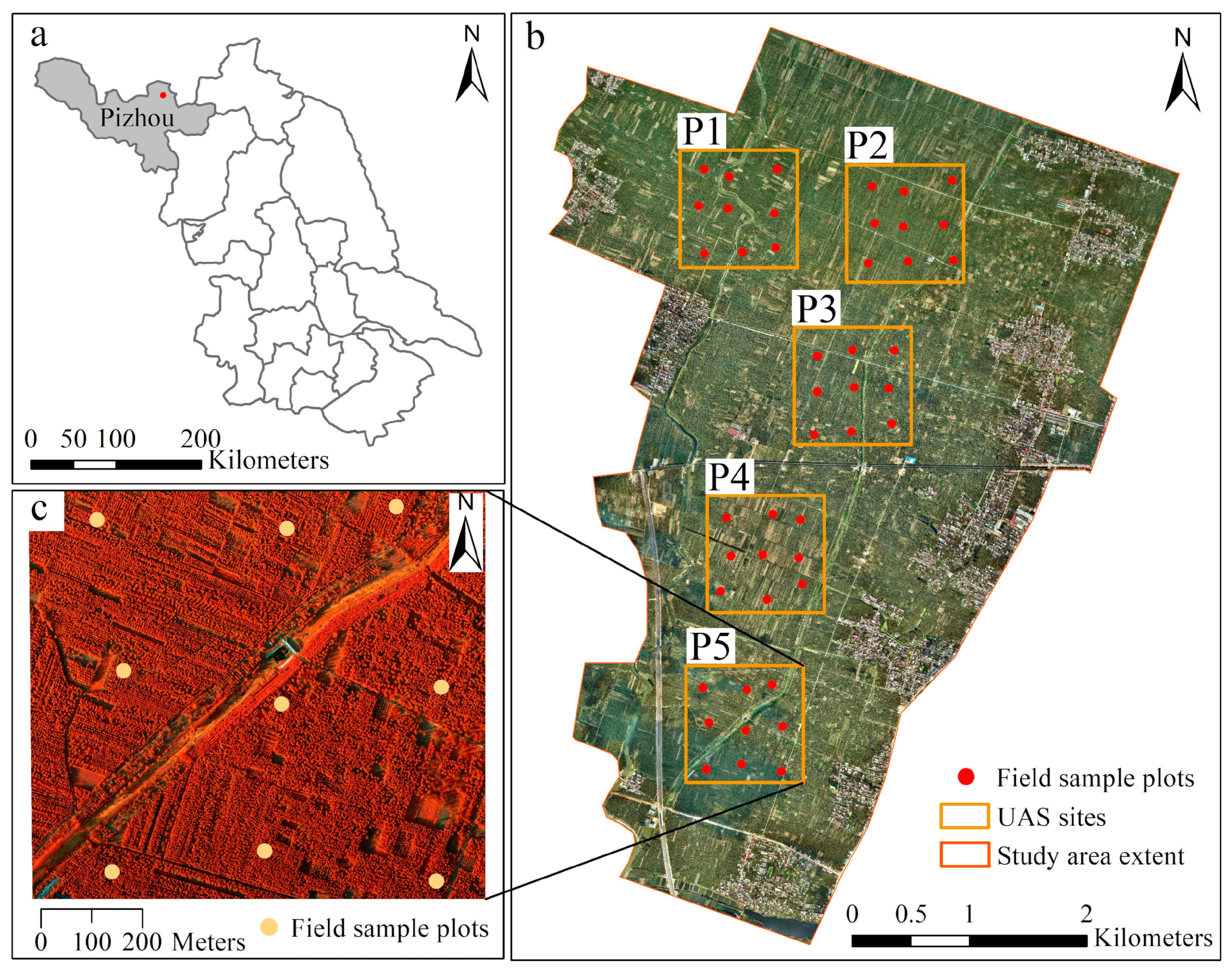
A general overview of the workflow for forest structural attribute estimation is shown in Figure 1. First, point clouds and ortho-imageries were generated from UAS-acquired raw multispectral and RGB imageries using the digital aerial photogrammetry (DAP) approach. Second, different suits of spectral and structural metrics, i.e., wide-band spectral indices and point cloud metrics, were extracted from spectral ortho-imageries and height normalized DAP point clouds, respectively. The spectral and structural metrics were analyzed and assessed using correlation analysis and the index of variable importance of projection (VIP). Moreover, the structural metrics extracted from UAS multispectral and RGB DAP point clouds were compared and assessed using correlation analysis. Finally, the selected important spectral and structural metrics were used to fit PLS regression models individually and in combination to estimate Lorey’s mean height (H_L) (the stand mean height weighted by basal area [44]) and volume(V) (a forest structural attribute caculated by diameter at breast height and tree height [45]). The number of components was selected using the standard error of 10-fold cross-validation, and the capability and synergetic effects of DAP-derived spectral and structural metrics in predicting forest structural attributes in various stem density forests were assessed. More detailed information can be seen in the following sections.

2.1. Study Area

This study was conducted at Pizhou ginkgo plantation, a forest managed by local government and residents, in the town of Tiefu in the northern plain of Jiangsu province (118°4′10″E, 34°32′19″N) (Figure 2). It covers approximately 2190 ha, with an elevation ranging between 29 m to 32 m above sea level. It is situated in the semi-humid continental climate zone with an annual mean temperature of 14.0 °C and annual mean precipitation of 867 mm. The planted ginkgo (Ginkgo biloba L.) trees in the plantation were managed in different silvicultural treatments and have different stem densities.

2.2. Field Data

In the study, inventory data of field sample plots were obtained from the forest survey in October 2016 (under a leaf-on condition). A total of 45 circular sample plots (radius = 15 m) were established within 5 of 1 × 1 km² square UAS sites (Figure 2b). These sample plots were designed to cover a range of stand densities, age classes, and site indices, and can be divided into three groups based on stem density: (i) low stem density plots (stem density < 500 N·ha⁻¹, n = 17); (ii) medium stem density plots (500 N·ha⁻¹ ≤ stem density < 650 N·ha⁻¹, n = 17); and (iii) high stem density plots (stem density ≥ 650 N·ha⁻¹, n = 11). The position of the center of the field plots was assessed by Trimble GeoXH6000 GPS units, corrected with high precision real-time differential signals received from the Jiangsu Continuously Operating Reference Stations (JSCORS), resulting in a sub-meter accuracy.

All the live trees within each plot that had a DBH > 5 cm were measured. The measurement of individual tree included position, tree top height, height to crown base, crown width in both cardinal directions, and crown density. DBH was measured using a diameter tape for all trees. The positions of trees were measured using an ultrasound-based Haglöf PosTex^® positioning instrument (Långsele, Sweden). Tree top heights were measured using a Vertex IV^® hypsometer (Långsele, Sweden). Crown widths were obtained as the average of two values measured along two perpendicular directions from the location of tree top. Moreover, the crown class, i.e., dominant, co-dominant, intermediate, and overtopped, were also recorded. The plot-level forest structural attributes, including DBH, H_L, N, G, and V, were calculated using the measured individual tree data. The general volume equation of ginkgo in Jiangsu province was used to calculate the volume of each individual tree. The volume of each individual tree was calculated according to the DBH and H measured in the field, and then summed to the plot-level volume. The summary of the field-measured forest structural attributes is provided in

Table 1. Summary statistics of field measured forest structural attributes in the study site (n = 45, radius = 15 m).

Forest Parameters	G1 (n = 17)		G2 (n = 17)		G3 (n = 11)
	Range	Mean ± SD	Range	Mean ± SD	Range	Mean ± SD
DBH	10.61–23.39	19.96 ± 3.13	10.15–20.82	17.72 ± 2.68	10.49–17.74	14.74 ± 2.74
HL	6.69–14.53	12.01 ± 1.85	6.93–14.60	11.23 ± 1.93	6.64–12.64	10.32 ± 2.15
N	311–495	430 ± 57	509–608	561 ± 36	679–1329	866 ± 209
G	13.89–57.51	44.01 ± 10.89	15.22–64.47	46.23 ± 12.90	20.29–74.82	48.58 ± 15.92
V	16.55–105.26	74.97 ± 21.95	18.50–120.86	76.16 ± 26.42	24.08–128.81	76.61 ± 31.61

DBH: diameter at breast height (cm); H_L: Lorey’s mean height (m); N: stem density (N·ha⁻¹); G: basal area (m²·ha⁻¹); V: volume (m³·ha⁻¹); SD: standard deviation; G1: stem density < 500 N·ha⁻¹; G2: 500 N·ha⁻¹ ≤ stem density ≤ 650 N·ha⁻¹; G3: stem density > 650 N·ha⁻¹.

.

2.3. Remote Sensing Data

High spatial resolution RGB and multispectral aerial imageries were acquired from a fixed-wing UAS on 21–24 September 2016. The acquisition was conducted in clear weather conditions. The RGB imagery covered the whole study area, and the multispectral imagery covered the five UAS sites (Figure 2). The detailed parameters of image acquisition were provided in

Table 2. Imagery acquisition parameters.

	MicaSense RedEdge	Sony A7R
Flight height (m)	150	350
Flight speed (m/s)	30	20
Forward overlap (%)	80	75
Lateral overlap (%)	80	65
Spectral bands	Blue, Green, Red, Red-edge and Near-infrared	Blue, Green and Red
Optimal resolution	1280 × 960	7360 × 4912
ground sample distance (cm)	10	5
Image format	16-bit TIFF (Tagged Image File Format)	24-bit TIFF

. A total of 47 three-dimensional ground control points (GCPs), which were distributed in the whole study area, were measured for UAS imagery geocorrection. The coordinates of three-dimensional GCPs were acquired by a Trimble R4 GNSS receiver, corrected with high precision real-time differential signals received from the Trimble NetR9 GNSS reference receiver. Horizontal and vertical accuracies of the GCPs were ±1 cm and 2 cm, respectively.

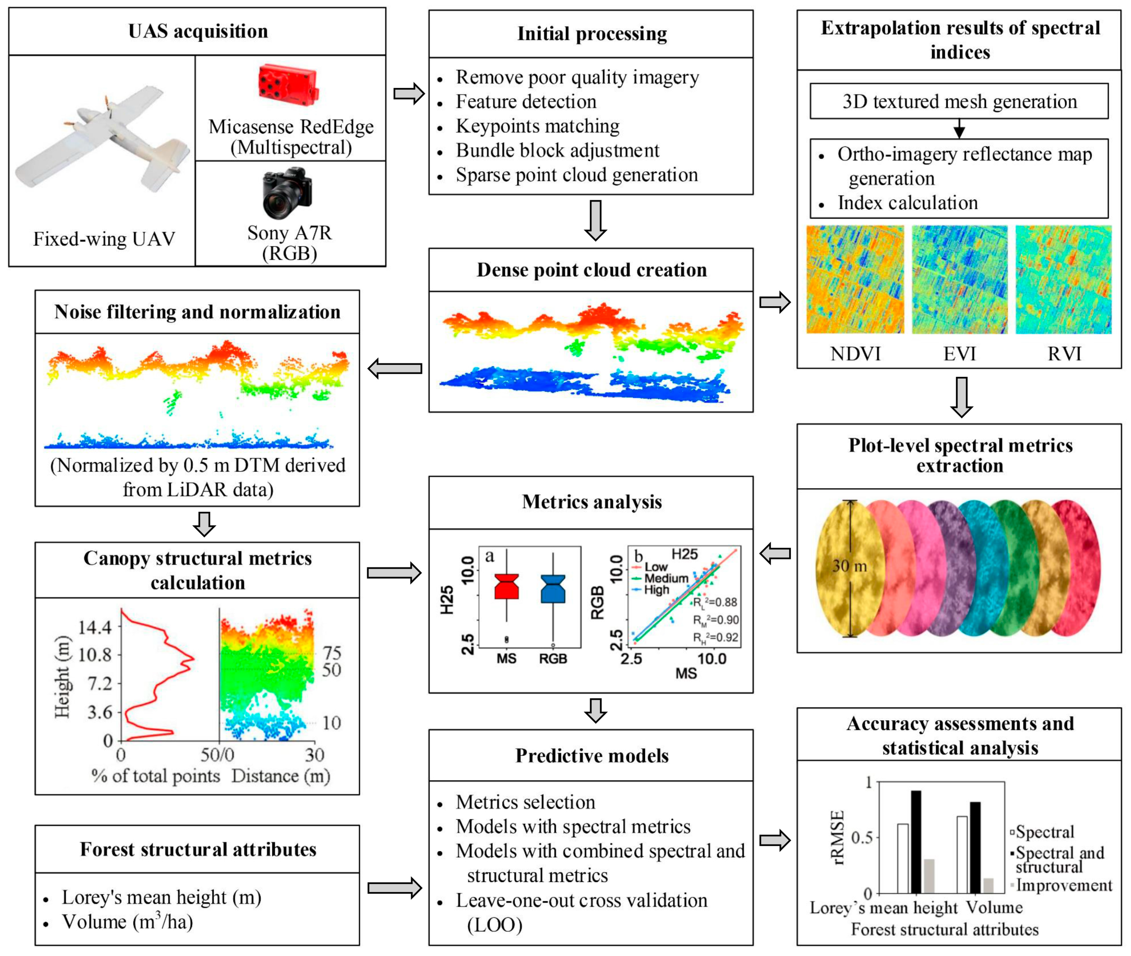
2.4. Data Pre-Processing

The RGB and multispectral images which have poor quality (i.e., the images acquired in turning points or not at the target altitude) were removed before data processing. The retained images were processed using the Pix4Dmapper Professional Edition (Pix4D, 2018). The module of initial processing was used in this stage. First, the binary descriptors in Hamming space were used to match keypoints (i.e., detected common features) between corresponding images. Second, the matched keypoints and the image position and orientation recorded in UAS were used in bundle block adjustment to calculate the exact exterior orientation parameters of the camera for each image. Finally, the three-dimensional coordinates of matched keypoints were calculated based on the intrinsic and extrinsic parameters of the camera and the coordinates of three-dimensional GCPs measured in the field. In the study, 30 GCPs were selected randomly as control points, and the other 17 GCPs were used as check points. Point cloud densitification was also conducted using the module of point cloud and mesh to obtain a dense point cloud, and the point density was set to high in order to maximize the density of point cloud. The dense point cloud was classified into ground and non-ground points using the filtering algorithm adapted from a previous study [46]. The DAP digital terrain model (DTM) was created by calculating the average elevation from the ground points within each cell, and the cells that contained no points were interpolated by linear interpolation of neighboring cells. The quality of created DAP DTM was assessed using the 17 check points, and the mean RMSE in the vertical direction was 0.023 m.

2.5. Point Cloud Processing

The dense DAP point cloud was filtered for noise before analysis. Then, the DAP point cloud was classified into the ground and non-ground points using a filtering algorithm adapted from a previous study [46]. Since the availability of ground points was limited, the 1 m DTM derived from LiDAR data (acquired using a multi-rotor UAV with lightweight Velodyne Puck VLP-16 sensor) was used to normalize the DAP point cloud. The 1 m digital surface model (DSM) was created using the points with maximum heights in each cell, and the cells that contained no point were interpolated by linear interpolation of neighboring cells.

The structural metrics derived from height normalized DAP point cloud were used to describe the structure of the forest canopy. In this study, a total of 15 structural metrics were extracted, including: (i) selected percentile heights (H25, H50, H75, and H95); (ii) selected canopy’s return density measures, i.e., canopy return densities (D1, D3, D5, D7, and D9); (iii) mean/maximum height (Hmean/Hmax) and coefficient of variation of heights (Hcv); (iv) canopy volume zones (open, E, O, and closed); and (v) weibull parameters fitted to the profile of apparent foliage density (W_α and W_β). A summary of the structural metrics and their descriptions is given in

Table 3. The summary of the structural metrics extracted from the digital aerial photogrammetry point cloud (the code and description of each metric are listed).

Metrics	Description
Percentile heights (H25, H50, H75, and H95)	The percentiles of the canopy height distributions (25th, 50th, 75th, and 95th)
Canopy return density (D1, D3, D5, D7, and D9)	The proportion of points above the quantiles (10th, 30th, 50th, 70th, and 90th) to total number of points
Mean/Maximum height (Hmean/Hmax)	Mean/maximum height above ground of all points
Coefficient of variation of heights (Hcv)	Coefficient of variation of heights of all points
Open and Closed gap zones of Canopy volume models (CVM) (i.e., Open and Closed)	The empty voxels located above and below the canopy
Euphotic and Oligophotic zones of CVM (i.e., E and O)	The voxels located within an uppermost percentile (65%) of all filled grid cells of that column, and voxels located below the point in the profile
α and β parameter of Weibull distribution (i.e., Wα and Wβ)	The α and β parameter of the Weibull distribution fitted to foliage density profile

.

2.6. Image Processing

The image processes were performed under the default settings of Pix4Dmapper modules, except the spatial resolution was set as highest. The dense point cloud was used to create a 3D textured mesh. Then, the ortho-imageries were generated using 3D textured mesh files and an orthorectification algorithm. In the process of imagery generation, the radiometric correction was conducted to remove the influences of sensor and illumination using the camera parameters and solar irradiance information. A suite of spectral metrics was calculated using the module of the index calculator. The spectral metrics of multispectral and RGB datasets were derived at 100 cm² (10 × 10 cm) and 25 cm² (5 × 5 cm), respectively. The mean of the spectral metrics in each plot was calculated to get the mean value of spectral metrics in the plot-level. A summary of the spectral metrics and their description is given in

Table 4. The summary of the vegetation indices with respective equations and reference.

Vegetation Index	Equation	Reference
Atmospherically Resistant Vegetation Index (ARVI)	(ρnir − ρrb)/(ρnir + ρrb), ρrb = ρred − γ (ρblue − ρred), γ=0.5	[47]
Difference Vegetation Index (DVI)	ρnir − ρred	[48]
Enhanced Vegetation Index (EVI)	2.5(ρnir − ρred)/(ρnir + 6ρred − 7.5ρblue +1)	[49]
Global Environment Monitoring Index (GEMI)	n(1 − 0.25n)(ρred − 0.125)/(1 − ρred), n = [2(ρnir2 − ρred2) + 1.5ρnir + 0.5ρred]/(ρnir + ρred + 0.5)	[50]
Green Normalized Difference Vegetation Index (GNDVI)	(ρnir − ρgreen)/(ρnir + ρgreen)	[50]
Infrared Percentage Vegetation Index (IPVI)	ρnir/(ρnir + ρred)	[51]
Red Green Ratio Index (RGRI)	ρred − ρgreen	[52]
Modified Soil Adjusted Vegetation Index (MSAVI)	[2ρnir + 1 − [(2ρnir + 1)2 − 8(ρnir − ρred)]0.5]/2	[53]
Modified Simple Ratio Vegetation Index (MSR)	ρred/(ρnir/ρred + 1)0.5	[53]
Modified Triangular Vegetation Index (MTVI)	[1.5(1.2(ρnir − ρgreen) − 2.5(ρred − ρgreen)]/[(2ρnir + 1)2 − (6ρnir − 5ρred0.5) − 0.5]0.5	[53]
Normalized Difference Vegetation Index (NDVI)	(ρnir − ρred)/(ρnir + ρred)	[53]
Optimized Soil Adjusted Vegetation Index (OSAVI)	(ρnir − ρred)/(ρnir + ρred + 0.16)	[54]
Renormalized Difference Vegetation Index (RDVI)	(ρnir − ρred)/(ρnir + ρred) 0.5	[53]
Ratio Vegetation Index (RVI)	ρred/ρnir	[55]
Soil and Atmospherically Resistant Vegetation Index (SARVI)	(1 + 0.5)(ρnir − ρrb)/(ρnir + ρrb + 0.5), ρrb = ρred − γ(ρblue -ρred), γ = 0.5	[53]
Soil Adjusted Vegetation Index (SAVI)	(1 + 0.5)(ρnir − ρred)/(ρnir + ρred + 0.5)	[53]
Simple Ration Vegetation Index (SR)	ρnir/ρred	[56]
Simple Ratio × Normalized Difference Vegetation Index (SR × NDVI)	(ρnir2 − ρred)/(ρnir + ρred2)	[57]
G/R (GR)	ρgreen/ρred	[58]
Brightness (BI)	ρgreen + ρred + ρblue	[58]
Normalized Greenness (Norm G)	ρgreen/(ρgreen + ρred + ρblue)	[58]
Normalized Green-Red Ratio (Norm GR)	(ρgreen − ρred)/(ρgreen + ρred)	[58]

Note: The vegetation indices were calculated using raw imagery bands; ρ_blue = Blue band, ρ_green = Green band, ρ_red = Red band, ρ_nir = Near infrared band.

.

2.7. Statistical Analysis and Modeling

The plot-level spectral and structural metrics derived from ortho-imageries (including multispectral and RGB imageries) and DAP point cloud (including multispectral and RGB DAP point clouds) were used as predictor variables to model forest structural attributes (i.e., Lorey’s mean height and Volume) in planted subtropical forests. The PLS regression modeling approach, which is commonly utilized to deal with the issue of multicollineariy of predictor variables and suitable for the situation of predictor variables more than observed samples [59,60,61,62], was used to fit predictive models of forest structural attributes. The PLS regression models assume that the variance in predictor variables can be represented by a few important components [63]. The information of dependent and independent variables are all transformed into features [64].

To improve the interpretability of metrics, all of the metrics were centered to have a mean of 0 and scaled to have a standard deviation of 1 before fitting PLS models [39]. Moreover, the variable importance of projection (VIP) [65], which represents the contribution or importance of each metric in fitting the PLS model, was calculated and used to evaluate the importance of each metric. The metrics with VIP higher than 0.8 were selected in the modeling of final predictive PLS models. The standard error of 10-fold cross-validation was used to select the optimal number of components in the predictive PLS models. The number of components with the lowest standard error was selected.

In the study, three types of predictive PLS models of Lorey’s mean height and Volume were fitted using spectral and structural metrics derived from ortho-imageries and DAP point clouds. First, the predictive PLS models of Lorey’s mean height and Volume were fitted using only spectral metrics extracted from either multispectral RGB ortho-imageries (i.e., the PLS models with multispectral-derived spectral metrics (PLS_MS-S), and with RGB-derived spectral metrics (PLS_RGB-S)). Second, the predictive models were fitted using combined spectral and structural metrics derived from either multispectral RGB dataset (i.e., the PLS models with multispectral-derived spectral and structural metrics (PLS_MS-CO), and with RGB-derived spectral and structural metrics (PLS_RGB-CO)). Finally, the spectral metrics derived from multispectral ortho-imagery and structural metrics derived from RGB DAP point cloud were combined to fit the combo models (PLS_MS-RGB) to predict the forest structural attributes of Lorey’s mean height and Volume in a planted subtropical forest. Moreover, to assess the capability of DAP-derived spectral and structural metrics in predicting forest structural attributes in various stem densities, the predictive models with different stem densities (i.e., low, medium, and high stem density) were fitted using stratified sample plots. The performance of predictive PLS models was assessed using a 10-fold cross validated coefficient of determination (R²), Root-Mean-Square Error (RMSE), and relative RMSE (rRMSE).

$$\mathrm{RMSE}=\sqrt{\frac{1}{\mathrm{n}}{\displaystyle \sum }_{\mathrm{i}=1}^{\mathrm{n}}{{(\mathrm{x}}_{\mathrm{i}}-\widehat{{\mathrm{x}}_{\mathrm{i}}})}^2}$$

(1)

$$r\mathrm{RMSE}=\frac{\mathrm{RMSE}}{\overline{x}}\times 100\%$$

(2)

where ${\mathrm{x}}_{\mathrm{i}}$ is the observed forest structural attributes (i.e., Lorey’s mean height and Volume) for the plot i, $\widehat{{\mathrm{x}}_{\mathrm{i}}}$ is the estimated forest structural attributes for the plot i, $\overline{x}$ is the mean value of observed forest structural attributes, and n is the number of plots.

3. Results

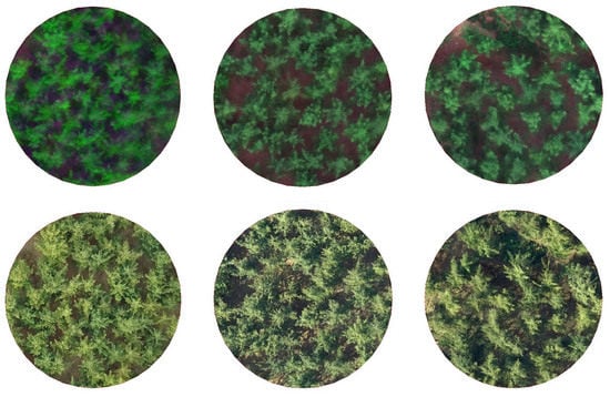
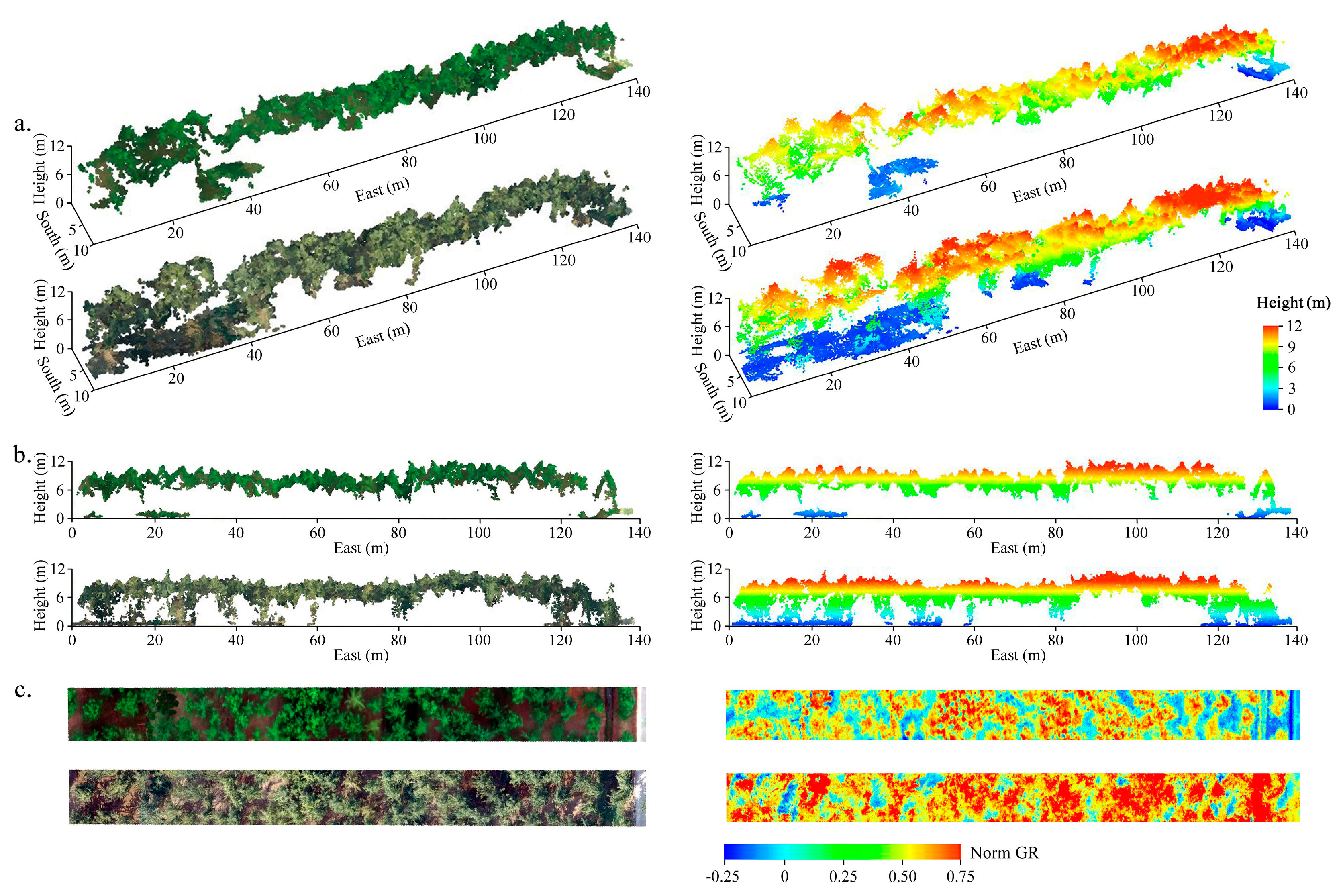
3.1. DAP Point Clouds and Reflectance Imageries Generation

The point clouds and reflectance imageries generated from multispectral and RGB imageries using digital aerial photogrammetry approach had the perfect visual effect (Figure 3). The three-dimensional structural and two-dimensional spectral information were recorded in detail. Although the UAS imagery only provided the two-dimensional information for the surface of the forest canopy, the information in the lower canopy could still be acquired while the canopy gaps were large enough. Moreover, the RGB imageries with higher spatial resolution than multispectral imageries provided more detailed 2D and 3D information for the forest structure (Figure 3a,c).

The point clouds and imageries in the plot-level also recorded detailed structural and spectral attributes of sample plots (Figure 4). For multispectral and RGB datasets, the point clouds and imageries in sample plots with different stem densities (i.e., low, medium, and high stem density plots) had different performances. The plot with higher stem density had less points in the ground and recorded less soil background information. Therefore, the stem density had an influence in point cloud distribution. Moreover, the height distributions of point clouds described the vertical distributions of canopy materials (Figure 4b,c). Most of the point clouds were concentrated in the forest canopy, and the plot with higher tree height had a higher peak for the distribution curve. The RGB DAP point cloud recorded more detailed structural information than the multispectral DAP point cloud. Compared with the RGB point cloud, points from the multispectral point cloud were more concentrated in the forest canopy. In addition, the RGB point cloud had more points in the lower canopy than the multispectral point cloud (Figure 4c).

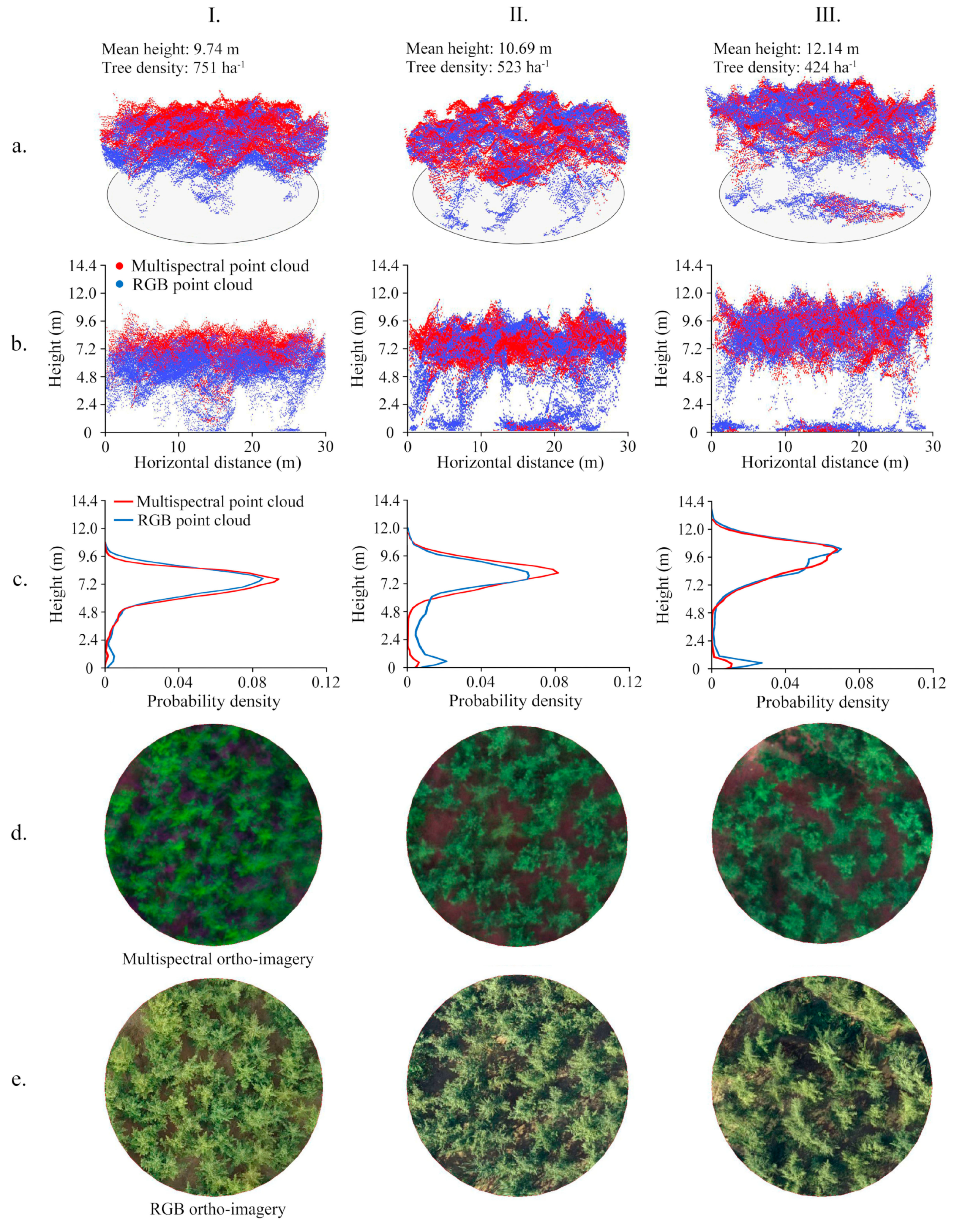
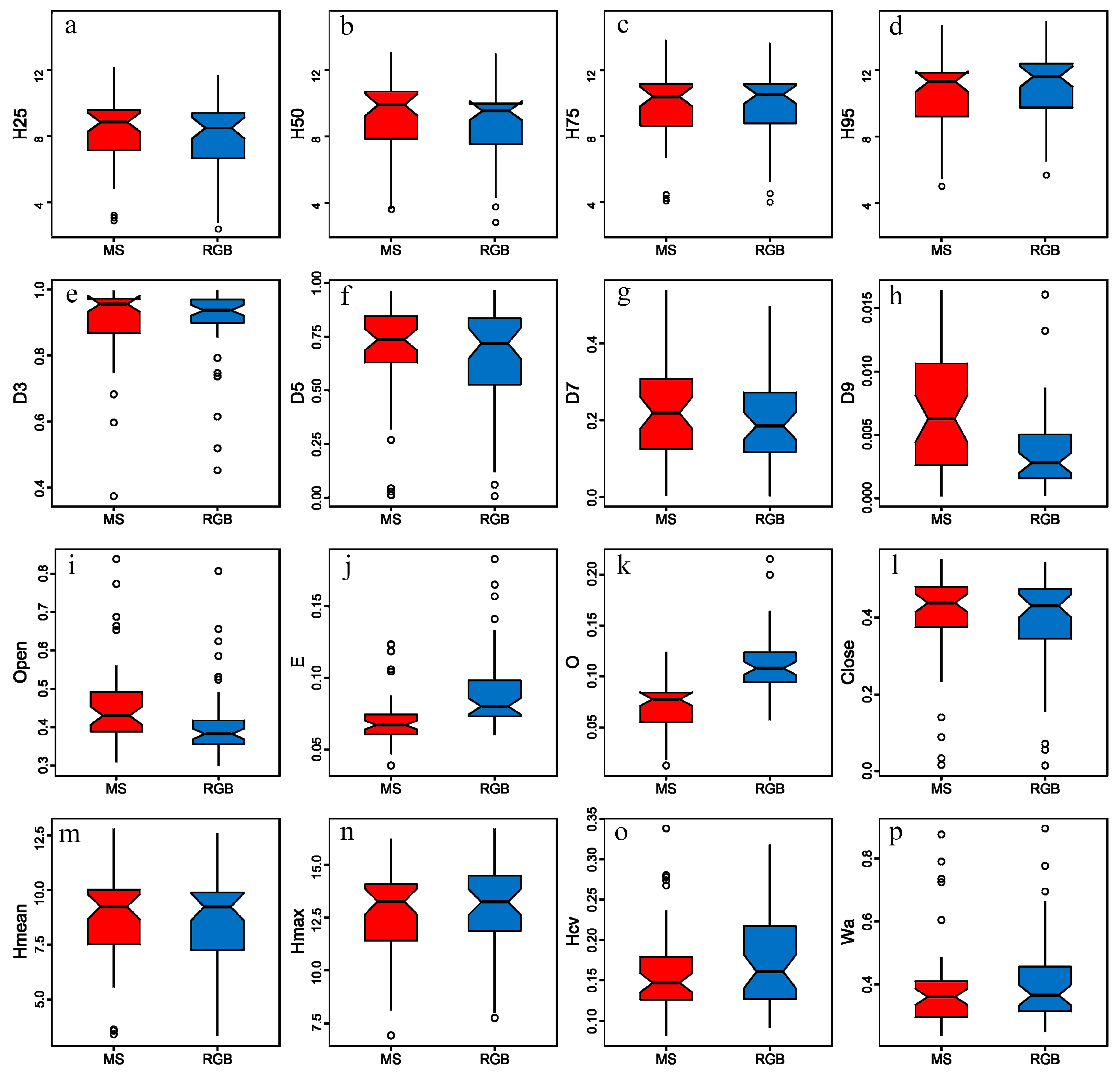
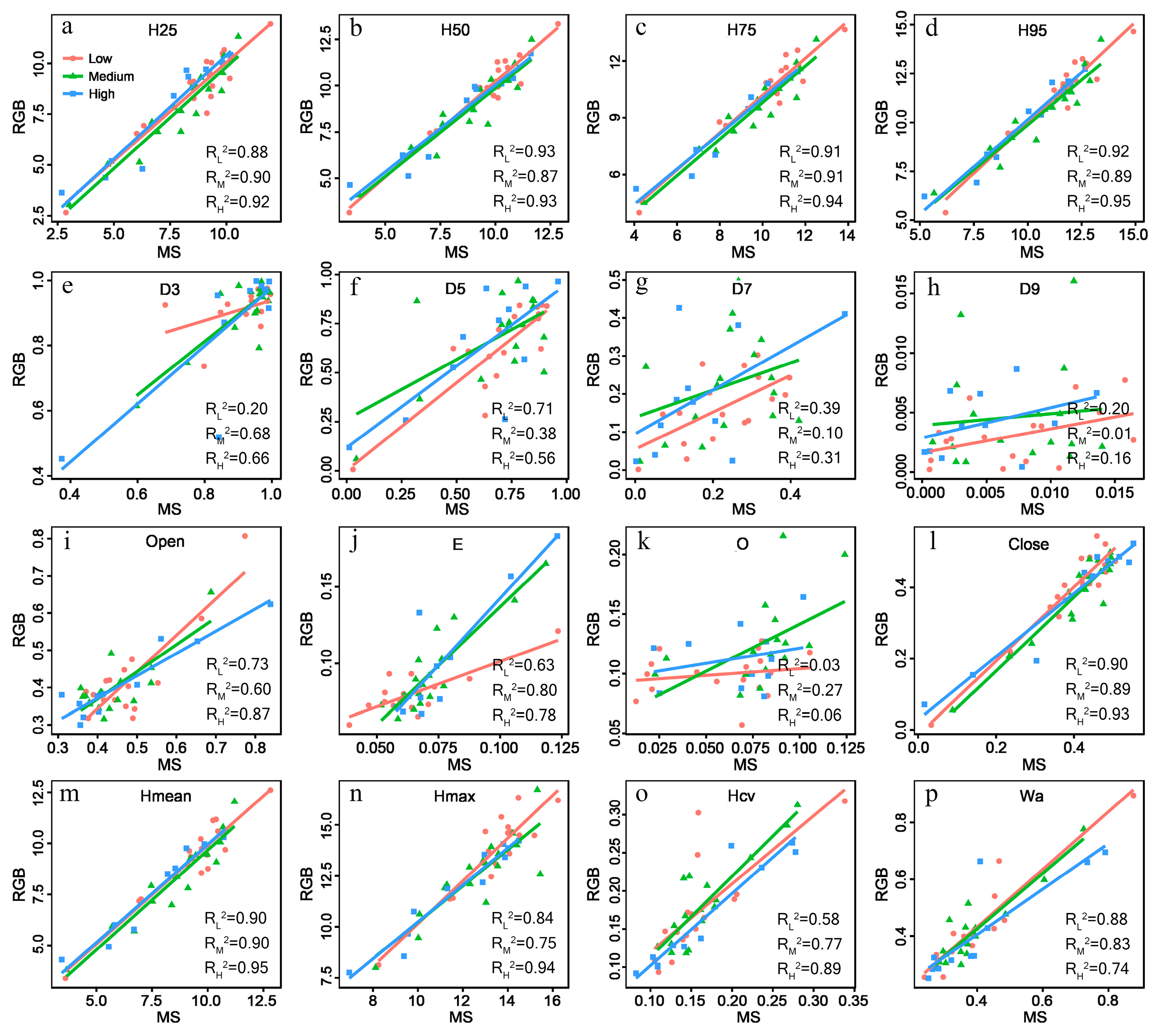
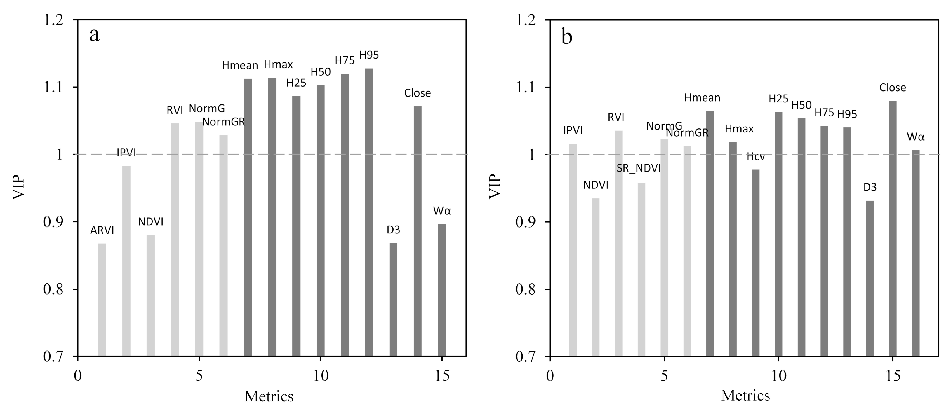
3.2. Structural Metrics Extraction and Analysis

The structural metrics extracted from DAP point clouds derived from multispectral and RGB imageries are shown in Figure 5. The structural metrics extracted from multispectral and RGB DAP point clouds were different. For percentile heights, the means of H25 and H50 of the multispectral DAP point cloud were higher than RGB DAP point cloud. However, the mean of H95 of the RGB DAP point cloud was higher than the multispectral DAP point cloud. For canopy return density, the means of D3, D5, D7, and D9 of the RGB DAP point cloud were all slightly lower than the multispectral DAP point cloud. For metrics of canopy volume models, the means of open and close for the multispectral DAP point cloud were higher than the RGB DAP point cloud. However, the means of E and O of the multispectral DAP point cloud were lower than the RGB DAP point cloud. For Hmean, the ranges and distributions of multispectral and RGB DAP point clouds were similar. For Hmax, Hcv and W_α, the ranges of the RGB DAP point cloud were higher than the multispectral DAP point cloud.

Moreover, the relationship between structural metrics derived from multispectral and RGB DAP point clouds were compared and assessed (Figure 6). Most of the structural metrics extracted from the multispectral DAP point cloud were highly correlated with the metrics derived from the RGB DAP point cloud (R² > 0.75). For percentile heights, metrics of H25, H50, H75, and H95 extracted from the multispectral DAP point cloud were all highly correlated with those from the RGB DAP point cloud (R² ≥ 0.87) (Figure 6a–d). In this study, all of the 45 sample plots were stratified into three groups (i.e., low, medium, and high stem density) to assess the influence of stem density on structural metrics. The percentile heights extracted from the multispectral DAP point cloud in high stem density plots had stronger correlations with those from the RGB DAP point cloud (Figure 6a–d). Moreover, the coefficient of determination (R²) of fitted models for structural metrics of Hmean (and Hcv) increased with increasing stem density (Figure 6m,o).

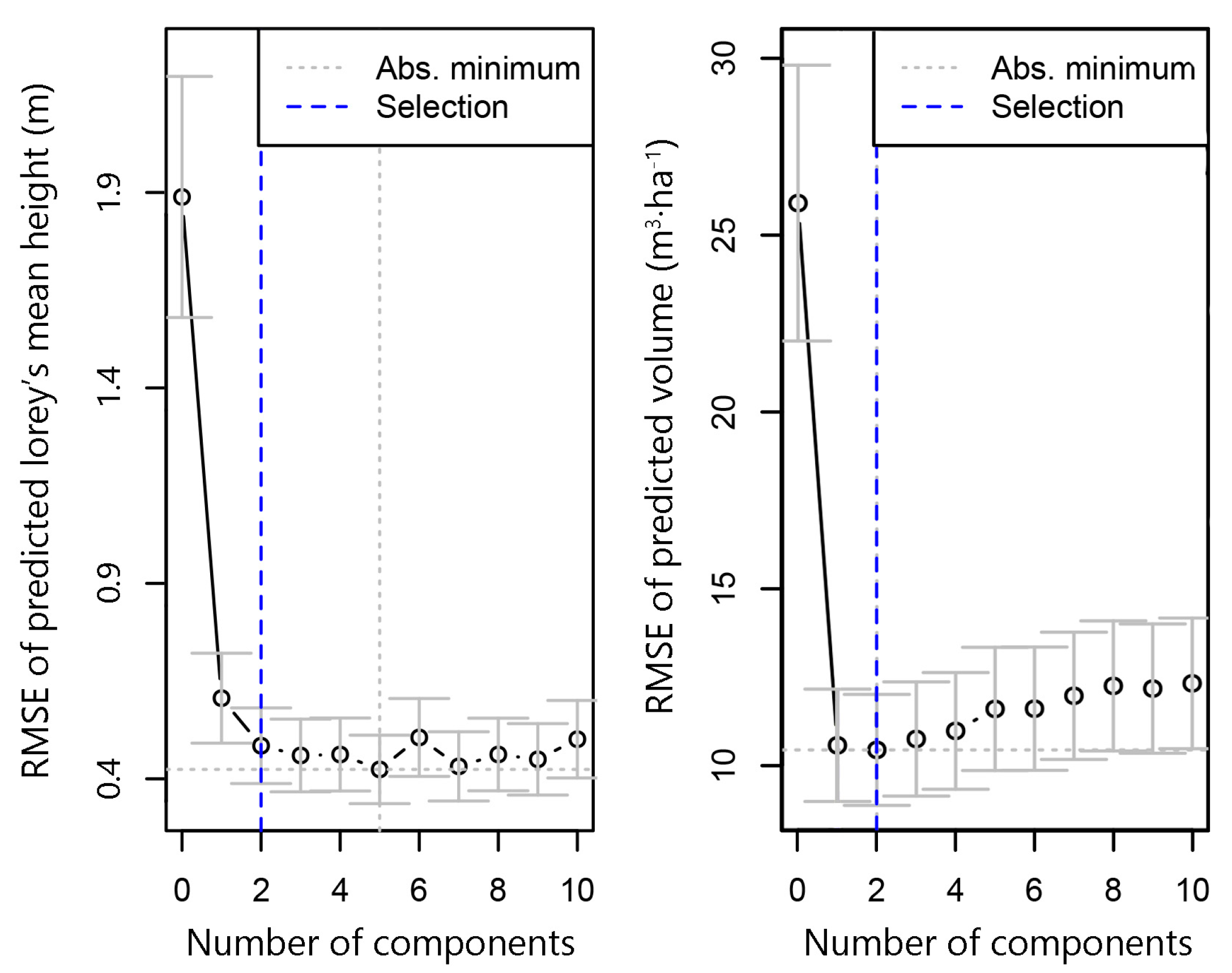
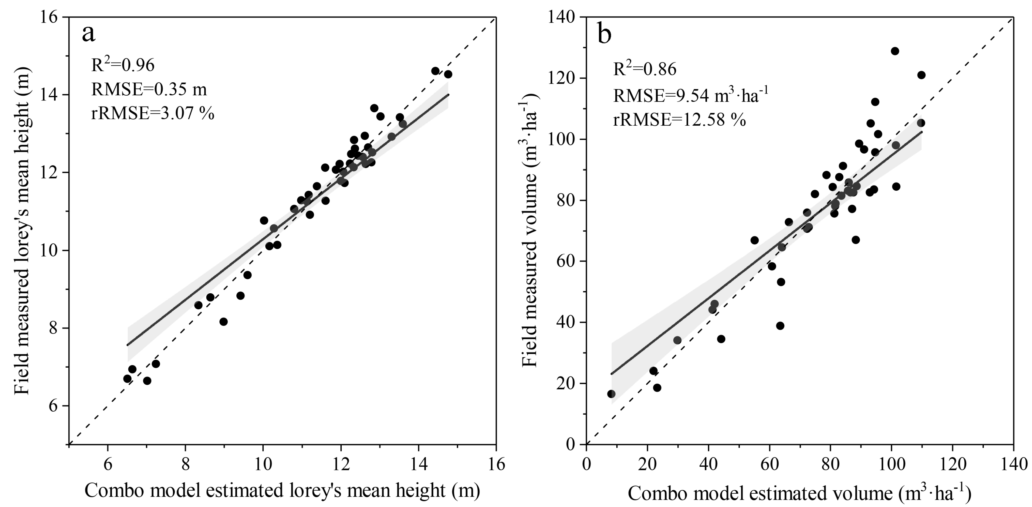
3.3. Forest Structural Attributes Modeling

The PLS models with spectral metrics and combined spectral and structural metrics extracted from multispectral imageries performed well in the modeling of forest structural attributes (

Table 5. Summary of the forest structural attribute prediction models with spectral and structural metrics derived from UAS multispectral imageries and the DAP point cloud. The best models based on the standard error of the cross-validation residuals are displayed with the number of components, total explained variability (%), cross-validated coefficient of determination (R2), cross-validated Root-Mean-Squared-Error (RMSE), and relative RMSE (rRMSE).

Models	Number of Components	Total Explained Variability (%)	R2	RMSE	rRMSE (%)
Spectral metrics
HLa	3	99.33	0.69	1.23	10.88
HLb	3	98.30	0.71	1.20	9.99
HLc	2	97.84	0.73	1.12	9.97
HLd	3	99.78	0.73	1.03	9.99
Va	2	95.99	0.62	14.14	18.65
Vb	2	96.09	0.64	13.95	18.61
Vc	3	98.08	0.70	13.50	17.73
Vd	2	98.50	0.69	13.62	17.78
Combined spectral and structural metrics
HLa	3	96.20	0.92	0.55	4.86
HLb	3	96.11	0.93	0.53	4.41
HLc	3	96.34	0.93	0.49	4.36
HLd	2	98.11	0.94	0.44	4.26
Va	2	94.43	0.82	11.06	14.59
Vb	3	97.85	0.84	10.74	14.33
Vc	3	96.75	0.85	10.72	14.08
Vd	3	97.95	0.87	10.16	13.26

Note: H_L = Lorey’s mean height (m); V = volume (m³·ha⁻¹); ^a predictive models fitted using all of the 45 sample plots; ^b predictive models fitted using 17 sample plots with low stem density; ^c predictive models fitted using 17 sample plots with medium stem density; ^d predictive models fitted using 11 sample plots with high stem density.

). The models fitted for all of the sample plots and stratified sample plots performed well (R² = 0.62–0.94, rRMSE = 4.26–18.65%). In general, the models fitted using combined spectral and structural metrics (R² = 0.82–0.94, rRMSE = 4.26–14.59%) were more accurate than those fitted using only spectral metrics (R² = 0.62–0.73, rRMSE = 9.97–18.65%). Moreover, the models fitted using stratified sample plots had relatively higher accuracies than those fitted using all of the sample plots (∆R² = 0.01–0.08, ∆rRMSE = 0.04–1.33%). The models of H_L fitted using only spectral metrics had accuracies from 0.69 (R², rRMSE = 10.88%) to 0.73 (R², rRMSE = 9.97%). The models of V fitted using only spectral metrics had accuracies from 0.62 (R², rRMSE = 18.65%) to 0.70 (R², rRMSE = 17.73%). The models of H_L fitted using combined spectral and structural metrics had accuracies from 0.92 (R², rRMSE = 4.86%) to 0.94 (R², rRMSE = 4.26%). The models of V fitted using combined spectral and structural metrics had accuracies from 0.82 (R², rRMSE = 14.59%) to 0.87 (R², rRMSE = 13.26%).

The PLS models with spectral metrics and combined spectral and structural metrics extracted from RGB imageries also had relatively high accuracy in estimation of forest structural attributes (

Table 6. Summary of the forest structural attributes prediction models with spectral and structural metrics derived from UAS RGB imageries and the DAP point cloud. The best models based on the standard error of the cross-validation residuals are displayed with the number of components, total explained variability (%), cross-validated coefficient of determination (R²), cross-validated Root-Mean-squared-Error (RMSE), and relative RMSE (rRMSE).

Models	Number of Components	Total Explained Variability (%)	R2	RMSE	rRMSE (%)
Spectral metrics
HLa	3	99.71	0.58	1.63	14.41
HLb	3	99.83	0.59	1.60	13.32
HLc	4	99.82	0.63	1.49	13.27
HLd	3	99.90	0.64	1.36	13.18
Va	4	99.84	0.56	16.62	21.92
Vb	3	99.85	0.60	15.99	21.33
Vc	3	94.40	0.61	15.87	20.84
Vd	2	92.73	0.60	16.17	21.10
Combined spectral and structural metrics
HLa	3	93.56	0.93	0.52	4.60
HLb	3	94.02	0.94	0.50	4.16
HLc	2	97.03	0.94	0.46	4.10
HLd	2	95.35	0.96	0.42	4.07
Va	4	93.18	0.82	10.74	14.17
Vb	3	93.33	0.84	10.61	14.15
Vc	2	92.91	0.85	10.52	13.81
Vd	3	94.47	0.88	9.82	12.82

Note: H_L = Lorey’s mean height (m); V = volume (m³·ha⁻¹); ^a predictive models fitted using all of the 45 sample plots; ^b predictive models fitted using 17 sample plots with low stem density; ^c predictive models fitted using 17 sample plots with medium stem density; ^d predictive models fitted using 11 sample plots with high stem density.

). The models fitted for all of the sample plots and stratified sample plots performed well (R² = 0.56–0.96, rRMSE = 4.07–21.92%). In general, the models fitted using combined spectral and structural metrics (R² = 0.82–0.96, rRMSE = 4.07–14.17%) were more accurate than those fitted using only spectral metrics (R² = 0.56–0.64, rRMSE = 13.18–21.92%). Moreover, the models fitted using stratified sample plots had relatively higher accuracies than those fitted using all of the sample plots (∆R² = 0.01–0.06, ∆rRMSE = 0.02–1.35%). The models of H_L fitted using only spectral metrics had accuracies from 0.58 (R², rRMSE = 14.41%) to 0.64 (R², rRMSE = 13.18%). The models of V fitted using only spectral metrics had accuracies from 0.56 (R², rRMSE = 21.92%) to 0.61 (R², rRMSE = 20.84%). The models of H_L fitted using combined spectral and structural metrics had accuracies from 0.93 (R², rRMSE = 4.60%) to 0.96 (R², rRMSE = 4.07%). The models of V fitted using combined spectral and structural metrics had accuracies from 0.82 (R², rRMSE = 14.17%) to 0.88 (R², rRMSE = 12.82%).

In the combo models fitted using the data from all of the sample plots, the number of components was two (Figure A1). The PLS combo models of forest structural attributes fitted using structural metrics derived from multispectral ortho-imageries and structural metrics derived from the RGB DAP point cloud had the best performance (

Table 7. Summary of the forest structural attributes prediction models with spectral metrics derived from the UAS multispectral imagery and structural metrics derived from the UAS RGB DAP point cloud. The best models based on the standard error of the cross-validation residuals are displayed with the number of components, total explained variability (%), cross-validated coefficient of determination (R²), cross-validated Root-Mean-squared-Error (RMSE), and relative RMSE (rRMSE).

Models	Number of Components	Total Explained Variability (%)	R2	RMSE	rRMSE (%)
HLa	2	97.72	0.94	0.48	4.24
HLb	2	95.53	0.94	0.45	3.75
HLc	2	94.46	0.96	0.34	3.03
HLd	2	97.95	0.97	0.30	2.91
Va	2	92.10	0.83	10.43	13.76
Vb	3	94.27	0.87	9.82	13.10
Vc	2	95.00	0.89	8.87	11.65
Vd	3	95.34	0.90	8.18	10.68

Note: H_L = Lorey’s mean height (m); V = volume (m³·ha⁻¹); ^a predictive models fitted using all of the 45 sample plots; ^b predictive models fitted using 17 sample plots with low stem density; ^c predictive models fitted using 17 sample plots with medium stem density; ^d predictive models fitted using 11 sample plots with high stem density.

). The models fitted using stratified sample plots had relatively higher accuracies than those fitted using all of the sample plots (∆R² = 0–0.07, ∆rRMSE = 0.49–3.08%). The models of H_L fitted using combined spectral and structural metrics had accuracies from 0.94 (R², rRMSE = 4.24%) to 0.97 (R², rRMSE = 2.91%). The models of V fitted using combined spectral and structural metrics had accuracies from 0.83 (R², rRMSE = 13.76%) to 0.90 (R², rRMSE = 10.68%).

Based on the VIP scores, the metric of H95 had the highest relative importance for H_L prediction, followed by H75 and Hmax; the spectral metrics had relatively low importance. In the prediction of V, the structural metrics had relatively higher importance than spectral metrics. The metric of Close had the highest relative importance, followed by Hmean and H25 (Figure 7). Moreover, the forest structural attributes predicted by comb models with these metrics were closer to those measured in the field (Figure A2). Therefore, these metrics performed well in the prediction of forest structural attributes.

4. Discussion

In this study, the spectral indices and point clouds derived from UAS-based multispectral and RGB imageries were used to estimate forest structural attributes in a planted subtropical forest. Previous studies have used UAS-based imagery to estimate forest structural attributes (

Table 8. Summary of the previous studies that estimated forest structural attributes based on imageries.

Platforms	Sensors	Study Area	Forest Types	Estimated Forest Attributes	Accuracy of Models (rRMSE %)	References
Mx-Sight	Panasonic Lumix DMC-GF1	Alcolea, Spain	Subtropical forest	Mean height	11.5	[67]
DJI S800	Sony NEX-5R	South and southeast of Prague, Czech Republic	Temperate forest	Mean height, Crown diameter	11.42–12.62 and 14.29–18.56	[21]
SenseFly eBee	Canon S110 NIR	Våler municipality, Norway	Boreal forest	HL, Dominate height, N, G, V	13.3, 3.5, 39.2, 15.4, and 14.5	[40]
DJI Phantom 4	1/2.3 CMOS	Oita, Japan	Temperate forest	HL, Mean height, Maximum height, V	6.65, 7.50, 6.17, and 20.02	[68]
-	Voxel UltraCamX	northern Vancouver Island, Canada	temperate rainforest	HL, G, V	14.00, 37.68, and 36.87	[29]
Gatewing X100	Ricoh GR3	village of Felenne, Belgium	Temperate forest	Dominate height	8.40	[66]

). Lisein et al. [66] used UAS imagery and a digital aerial photogrammetry approach to estimate dominant tree height in a temperate broadleaved forest, and the result showed that the dominant tree height was estimated with high accuracy (rRMSE = 8.40%). White et al. [29] used a UAS-based point cloud to estimate forest structural attributes in the coastal temperate rainforest, and they found that the Lorey’s mean height and volume were accurately estimated (rRMSE = 14.00% and 36.87%). Comparing to the results of this study with previous studies, the predictive models all had a relatively high accuracy. Moreover, the estimation of forest structural attributes in this study had a higher accuracy than most of the previous studies. This may be due to the fact that many structural metrics were extracted and the volume of low-lying vegetation under the forest canopy of the ginkgo plantation was less in this study. However, most of the previous studies focused on using a derived point cloud to estimate forest structural attributes, and estimation using combined spectral and structural metrics was rare. Puliti et al. [40] combined spectral and structural metrics to estimate Lorey’s mean height in a conifer-dominated boreal forest, and the rRMSE of predictive model was 13.28%. The estimation using UAS-based spectral and structural metrics in a planted subtropical forest was also comparable to those of the conifer-dominated boreal forest and temperate forest. In this study, the accuracy of the combo model was slightly higher than that of previous studies. The reason may be that the DTM derived from UAS-based LiDAR was used to normalize DAP point clouds.

Previous studies have found that the point density of the DAP point cloud is dependent on image resolution and matching algorithm [69,70]. Compared with DAP point clouds derived from UAS-based multispectral and RGB imageries, the RGB point cloud provided more detailed three-dimensional information about the forest structure. Visually, the number of points from the RGB DAP point cloud in the middle and lower canopy was greater than from the multispectral DAP point cloud (Figure 3 and Figure 4b). Moreover, the height distributions of the multispectral DAP point cloud and the RGB DAP point cloud were different (Figure 4c). In the upper canopy, the distributions were similar. However, more RGB DAP points were distributed in the lower canopy. Although the UAS imageries lacked penetration, lower canopy information can be recorded with a high spatial resolution sensor. Therefore, the RGB imagery with higher spatial resolution produced point cloud data with more detailed information of the forest structure.

The structural metrics derived from the multispectral DAP point cloud and RGB DAP point cloud were compared and assessed. For percentile heights, the means for H25 and H50 of the multispectral DAP point cloud were higher than the RGB DAP point cloud. However, the mean for H95 of the RGB DAP point cloud was higher than the multispectral DAP point cloud. For canopy return density, the means of D3, D5, D7, and D9 of the RGB DAP point cloud were all slightly lower than the multispectral DAP point cloud. For metrics of canopy volume models, the means of open and close for the multispectral DAP point cloud were higher than the RGB DAP point cloud. However, the means of E and O for the multispectral DAP point cloud were lower than the RGB DAP point cloud. These differences were caused by the distribution of the point clouds. The RGB DAP point cloud recorded more detailed three-dimension information of the forest structure than the multispectral DAP point cloud (Figure 3 and Figure 4b). Perroy et al. [71] used UAS-based imagery to assess the impacts of canopy openness on detecting sub-canopy plants in a tropical rainforest, and found that the detection rate for sub-canopy plants was 100% when above-crown openness values were higher than 40%. Therefore, the middle and lower canopy information can be recorded by DAP point cloud. In this study, the RGB DAP point cloud recorded more information for the middle and lower canopy than the multispectral DAP point cloud, and most of the points of the multispectral DAP point cloud were distributed in the upper canopy. Previous studies have found that the photogrammetry point cloud can underestimate tree height relative to field measurement [69,72]. This phenomenon was also found in this study. The individual tree height acquired from the DAP point clouds and measured in the field were compared. The result showed that the individual tree heights acquired from DAP point clouds were lower than those measured in the field (Figure 8). Moreover, the bias of underestimation for the multispectral DAP point cloud was larger than the RGB DAP point cloud (Figure 8). Therefore, the Hmax of the RGB DAP point cloud was larger than the multispectral DAP point cloud (Figure 5n). For the relationship between structural metrics derived from multispectral and RGB DAP point clouds, metrics of H25, H50, H75, H95, Close, Hmean, Hmax, Hcv, and W_α for the multispectral DAP point cloud were all highly correlated with the metrics of the RGB DAP point cloud (R² = 0.58–0.95). This means that these metrics extracted from multispectral and RGB DAP point clouds were similar, and the two DAP point clouds had similar capabilities in characterizing the three-dimensional structure of the forest. They can be interchanged with each other for estimation of forest structural attributes.

Spectral metrics, which are related to vegetation pigments, physiology, and stress, have great advantages in the estimation of forest structural attributes. In this study, a suite of vegetation indices was extracted to estimate forest structural attributes. The spectral metrics of IPVI, RVI, Norm G, and Norm GR were selected in the combo models. The red and near-infrared regions of the spectrum were sensitive to canopy biophysical properties [73,74,75]. IPVI and RVI were calculated using red and near-infrared bands, and Pearson and Miller [76] have found that RVI can slow down the rate of saturation under high canopy coverage. Therefore, the IPVI and RVI performed well in the estimation of forest structural attributes. The green band was thought to be correlated with vegetation pigment, nitrogen, and biomass [77,78,79], which was commonly used in the estimation of forest structural attributes [40,80]. Puliti et al. [40] found that the green band was more important than other bands in the estimation of forest structural attributes. In the combo models, Norm G and Norm GR were selected and showed good performances (rRMSE = 4.24 and 13.76%).

Structural metrics extracted from point cloud data are significantly related to forest structural properties. In this study, the accuracy of estimation models showed great improvement after using spectral and structural metrics (Table 5 and Table 6). In the combo models, metrics of percentile heights, Hmean, and Hmax were selected as important metrics. Thomas et al. [81] found that the structural metrics of H50 and H75 were strongly related to mean dominated height and basal area, and Stepper et al. [82] reported that Hmax had the highest correlation with field-measured tree top height. Therefore, the height-related metrics were most important in estimation of forest structural attributes in this study.

The combined use of spectral and structural metrics had a positive synergetic effect for the estimation of forest structural attributes. The models including only spectral metrics had the capability to predict forest structural attributes with relatively high accuracies (R² = 0.56–0.69, relative RMSE = 10.88–21.92%). However, the models with spectral and structural metrics had higher accuracies (R² = 0.82–0.93, relative RMSE = 4.60–14.17%). Therefore, the combination of spectral and structural metrics was realistic for improving the estimation accuracy of forest structural attributes. Compared to the models of multispectral and RGB UAS datasets, the accuracy improvements of RGB combined models were larger than those of multispectral combined models. This may be due to the many advanced spectral metrics being extracted from multispectral UAS imagery causing the spectral models to have relatively higher accuracies. Therefore, the improvement of multispectral combined models was limited. Nevertheless, the accuracies of combined models of multispectral and RGB UAS datasets were close. This means that the multispectral and RGB UAS datasets had similar capability to estimate forest structural attributes in planted subtropical forests. In addition, the models that combined used spectral metrics derived from the UAS multispectral imagery and structural metrics derived from the UAS RGB DAP point cloud had the highest accuracy (Table 7). Therefore, advanced spectral indices and detailed point cloud data can improve the accuracy of estimation of forest structural attributes.

Stem density is one of the key indicators for planted forest silviculture and sustainable management. In this study, the capability of DAP-derived spectral and structural metrics to predict forest structural attributes in various stem densities was assessed. The result indicated that predictive models fitted using stratified sample plots had relatively higher accuracies than those fitted using all of the sample plots (∆R² = 0–0.07, ∆rRMSE = 0.49–3.08%). Moreover, the estimation accuracies increased with increasing stem density. This may be caused by the loss of tree tops in the DAP point cloud generation [72]. When the surface of the forest canopy was uneven, the tree top information may be lost from the DAP point cloud. On the contrary, when the surface of the forest canopy was smooth, the tree tops may exist in the DAP point cloud. In this study, the forest with high stem density had a relatively smooth surface, and the forest with low stem density had an uneven surface. Therefore, the points of tree tops were easy to lose in the low stem density forest. This phenomenon was proven in Figure 8, where the difference in the low stem density forest between individual tree heights measured in the field and acquired in the DAP point cloud was the largest, and the difference in the high stem density forest was the lowest.

5. Conclusions

In this study, UAS-based multispectral and RGB imageries were used to estimate forest structural attributes in planted subtropical forests. The point clouds were generated from multispectral and RGB imageries using the DAP approaches. Different suits of multispectral- and RGB-derived spectral and structural metrics, i.e., wide-band spectral indices and point cloud metrics, were extracted, compared, and assessed using the index of VIP. The selected spectral and structural metrics were used to fit PLS regression models individually and in combination to estimate forest structural attributes (i.e., Lorey’s mean height (H_L) and volume(V)), and the capabilities of multispectral- and RGB-derived spectral and structural metrics in predicting forest structural attributes in various stem density forests were assessed and compared. The results indicated that most of the structural metrics extracted from the multispectral DAP point cloud were highly correlated with the metrics derived from the RGB DAP point cloud (R² > 0.75). In combo models, the estimation of H_L (R² = 0.94, relative RMSE = 4.24%) had a relatively higher accuracy than V (R² = 0.83, relative RMSE = 13.76%). Although the models including only spectral indices had the capability to predict forest structural attributes with relatively high accuracies (R² = 0.56–0.69, relative RMSE = 10.88–21.92%), the models with spectral and structural metrics had higher accuracies (R² = 0.82–0.93, relative RMSE = 4.60–14.17%). Moreover, the models fitted using RGB-derived spectral metrics had relatively lower accuracies than those fitted using multispectral-derived spectral metrics, but the models fitted using combined spectral and structural metrics derived from multispectral and RGB imageries had similar accuracies. In addition, the combo models fitted with stratified sample plots had relatively higher accuracies than those fitted with all of the sample plots (∆R² = 0–0.07, ∆ relative RMSE = 0.49–3.08%), and the accuracies increased with increasing stem density.

References

1. Food and Agriculture Organization. Global Forest Resources Assessment 2015—How Are the World’s Forests Changing? FAO: Rome, Italy, 2015; ISBN 9789251092835. [Google Scholar]
2. Kollert, W.; Liu, S.; Payn, T.; Carnus, J.-M.; Silva, L.N.; Freer-Smith, P.; Orazio, C.; Rodriguez, L.; Wingfield, M.J.; Kimberley, M. Changes in planted forests and future global implications. For. Ecol. Manag. 2015, 352, 57–67. [Google Scholar] [CrossRef] [Green Version]
3. Carnus, J.-M.; Parrotta, J.A.; Brockerhoff, E.G.; Arbez, M.; Jactel, H.; Kremer, A.; Lamb, D.; O’Hara, K.; Walters, B. Planted forests and biodiversity. J. For. 2006, 104, 65–77. [Google Scholar] [CrossRef]
4. Brin, A.; Payn, T.W.; Paquette, A.; Brockerhoff, E.G.; Pawson, S.M.; Parrotta, J.A.; Lamb, D. Plantation forests, climate change and biodiversity. Biodivers. Conserv. 2013, 22, 1203–1227. [Google Scholar] [CrossRef]
5. Spies, T. A Forest Structure: A Key to the Ecosystem. Northwest Sci. 1998, 72, 34–39. [Google Scholar] [CrossRef]
6. Van Leeuwen, M.; Nieuwenhuis, M. Retrieval of forest structural parameters using LiDAR remote sensing. Eur. J. For. Res. 2010, 129, 749–770. [Google Scholar] [CrossRef]
7. Wulder, M.A.; White, J.C.; Nelson, R.F.; Næsset, E.; Ørka, H.O.; Coops, N.C.; Hilker, T.; Bater, C.W.; Gobakken, T. Lidar sampling for large-area forest characterization: A review. Remote Sens. Environ. 2012, 121, 196–209. [Google Scholar] [CrossRef] [Green Version]
8. Zhao, M.; Zhou, G.S. Estimation of biomass and net primary productivity of major planted forests in China based on forest inventory data. For. Ecol. Manag. 2005, 207, 295–313. [Google Scholar] [CrossRef]
9. Tomppo, E.; Hagner, O.; Katila, M.; Olsson, H.; Ståhl, G.; Nilsson, M. Combining national forest inventory field plots and remote sensing data for forest databases. Remote Sens. Environ. 2008, 112, 1982–1999. [Google Scholar] [CrossRef]
10. Andersen, H.-E.; Reutebuch, S.E.; McGaughey, R.J. A rigorous assessment of tree height measurements obtained using airborne lidar and conventional field methods. Can. J. Remote Sens. 2006, 32, 355–366. [Google Scholar] [CrossRef]
11. Foody, G.M. Remote sensing of tropical forest environments: Towards the monitoring of environmental resources for sustainable development. Int. J. Remote Sens. 2003, 24, 4035–4046. [Google Scholar] [CrossRef] [Green Version]
12. McRoberts, R.E.; Tomppo, E.O. Remote sensing support for national forest inventories. Remote Sens. Environ. 2007, 110, 412–419. [Google Scholar] [CrossRef]
13. Meng, Q.; Cieszewski, C.; Madden, M. Large area forest inventory using Landsat ETM+: A geostatistical approach. ISPRS J. Photogramm. Remote Sens. 2009, 64, 27–36. [Google Scholar] [CrossRef]
14. Shataee, S.; Kalbi, S.; Fallah, A.; Pelz, D. Forest attribute imputation using machine-learning methods and ASTER data: Comparison of k-NN, SVR and random forest regression algorithms. Int. J. Remote Sens. 2012, 33, 6254–6280. [Google Scholar] [CrossRef]
15. Christensen, B.R. Use of UAV or remotely piloted aircraft and forward-looking infrared in forest, rural and wildland fire management: Evaluation using simple economic analysis. N. Z. J. For. Sci. 2015, 45, 16. [Google Scholar] [CrossRef]
16. Otero, V.; Van De Kerchove, R.; Satyanarayana, B.; Martínez-Espinosa, C.; Fisol, M.A.B.; Ibrahim, M.R.B.; Sulong, I.; Mohd-Lokman, H.; Lucas, R.; Dahdouh-Guebas, F. Managing mangrove forests from the sky: Forest inventory using field data and Unmanned Aerial Vehicle (UAV) imagery in the Matang Mangrove Forest Reserve, peninsular Malaysia. For. Ecol. Manag. 2018, 411, 35–45. [Google Scholar] [CrossRef]
17. Torresan, C.; Berton, A.; Carotenuto, F.; Di Gennaro, S.F.; Gioli, B.; Matese, A.; Miglietta, F.; Vagnoli, C.; Zaldei, A.; Wallace, L. Forestry applications of UAVs in Europe: A review. Int. J. Remote Sens. 2017, 38, 2427–2447. [Google Scholar] [CrossRef]
18. Goodbody, T.R.H.; Coops, N.C.; Marshall, P.L.; Tompalski, P.; Crawford, P. Unmanned aerial systems for precision forest inventory purposes: A review and case study. For. Chron. 2017, 93, 71–81. [Google Scholar] [CrossRef] [Green Version]
19. Colomina, I.; Molina, P. Unmanned aerial systems for photogrammetry and remote sensing: A review. ISPRS J. Photogramm. Remote Sens. 2014, 92, 79–97. [Google Scholar] [CrossRef] [Green Version]
20. Wallace, L.; Lucieer, A.; Watson, C.; Turner, D. Development of a UAV-LiDAR system with application to forest inventory. Remote Sens. 2012, 4, 1519–1543. [Google Scholar] [CrossRef]
21. Panagiotidis, D.; Abdollahnejad, A.; Surový, P.; Chiteculo, V. Determining tree height and crown diameter from high-resolution UAV imagery. Int. J. Remote Sens. 2017, 38, 2392–2410. [Google Scholar] [CrossRef]
22. Wallace, L.O.; Lucieer, A.; Watson, C.S. Assessing the Feasibility of Uav-Based Lidar for High Resolution Forest Change Detection. ISPRS Int. Arch. Photogramm. Remote Sens. Spat. Inf. Sci. 2012, XXXIX-B7, 499–504. [Google Scholar] [CrossRef]
23. Zahawi, R.A.; Dandois, J.P.; Holl, K.D.; Nadwodny, D.; Reid, J.L.; Ellis, E.C. Using lightweight unmanned aerial vehicles to monitor tropical forest recovery. Biol. Conserv. 2015, 186, 287–295. [Google Scholar] [CrossRef] [Green Version]
24. Chianucci, F.; Disperati, L.; Guzzi, D.; Bianchini, D.; Nardino, V.; Lastri, C.; Rindinella, A.; Corona, P. Estimation of canopy attributes in beech forests using true colour digital images from a small fixed-wing UAV. Int. J. Appl. Earth Obs. Geoinf. 2016, 47, 60–68. [Google Scholar] [CrossRef] [Green Version]
25. Granholm, A.H.; Lindgren, N.; Olofsson, K.; Nyström, M.; Allard, A.; Olsson, H. Estimating vertical canopy cover using dense image-based point cloud data in four vegetation types in southern Sweden. Int. J. Remote Sens. 2017, 38, 1820–1838. [Google Scholar] [CrossRef]
26. Guerra-Hernández, J.; González-Ferreiro, E.; Sarmento, A.; Silva, J.; Nunes, A.; Correia, A.C.; Fontes, L.; Tomé, M.; Díaz-Varela, R. Using high resolution UAV imagery to estimate tree variables in Pinus pinea plantation in Portugal. For. Syst. 2016, 25, eSC09. [Google Scholar] [CrossRef]
27. Rahlf, J.; Breidenbach, J.; Solberg, S.; Astrup, R. Forest parameter prediction using an image-based point cloud: A comparison of semi-ITC with ABA. Forests 2015, 6, 4059–4071. [Google Scholar] [CrossRef]
28. Saarinen, N.; Vastaranta, M.; Näsi, R.; Rosnell, T.; Hakala, T.; Honkavaara, E.; Wulder, M.; Luoma, V.; Tommaselli, A.; Imai, N.; et al. Assessing Biodiversity in Boreal Forests with UAV-Based Photogrammetric Point Clouds and Hyperspectral Imaging. Remote Sens. 2018, 10, 338. [Google Scholar] [CrossRef]
29. White, J.C.; Stepper, C.; Tompalski, P.; Coops, N.C.; Wulder, M.A. Comparing ALS and image-based point cloud metrics and modelled forest inventory attributes in a complex coastal forest environment. Forests 2015, 6, 3704–3732. [Google Scholar] [CrossRef]
30. Goodbody, T.R.H.; Coops, N.C.; Tompalski, P.; Crawford, P.; Day, K.J.K. Updating residual stem volume estimates using ALS- and UAV-acquired stereo-photogrammetric point clouds. Int. J. Remote Sens. 2017, 38, 2938–2953. [Google Scholar] [CrossRef]
31. White, J.C.; Coops, N.C.; Wulder, M.A.; Vastaranta, M.; Hilker, T.; Tompalski, P. Remote Sensing Technologies for Enhancing Forest Inventories: A Review. Can. J. Remote Sens. 2016, 42, 619–641. [Google Scholar] [CrossRef]
32. Gini, R.; Passoni, D.; Pinto, L.; Sona, G. Use of unmanned aerial systems for multispectral survey and tree classification: A test in a park area of northern Italy. Eur. J. Remote Sens. 2014, 47, 251–269. [Google Scholar] [CrossRef]
33. Salo, H.; Tirronen, V.; Pölönen, I.; Tuominen, S.; Balazs, A.; Heikkilä, J.; Saari, H. Methods for estimating forest stem volumes by tree species using digital surface model and CIR images taken from light UAS. Proc. SPIE 2012, 8390. [Google Scholar] [CrossRef]
34. Puliti, S.; Gobakken, T.; Ørka, H.O.; Næsset, E. Assessing 3D point clouds from aerial photographs for species-specific forest inventories. Scand. J. For. Res. 2017, 32, 68–79. [Google Scholar] [CrossRef]
35. Dempewolf, J.; Nagol, J.; Hein, S.; Thiel, C.; Zimmermann, R. Measurement of within-season tree height growth in a mixed forest stand using UAV imagery. Forests 2017, 8, 231. [Google Scholar] [CrossRef]
36. Melin, M.; Korhonen, L.; Kukkonen, M.; Packalen, P. Assessing the performance of aerial image point cloud and spectral metrics in predicting boreal forest canopy cover. ISPRS J. Photogramm. Remote Sens. 2017, 129, 77–85. [Google Scholar] [CrossRef]
37. Kalacska, M.; Sanchez-Azofeifa, G.A.; Rivard, B.; Caelli, T.; White, H.P.; Calvo-Alvarado, J.C. Ecological fingerprinting of ecosystem succession: Estimating secondary tropical dry forest structure and diversity using imaging spectroscopy. Remote Sens. Environ. 2007, 108, 82–96. [Google Scholar] [CrossRef]
38. Clark, M.L.; Roberts, D.A.; Ewel, J.J.; Clark, D.B. Estimation of tropical rain forest aboveground biomass with small-footprint lidar and hyperspectral sensors. Remote Sens. Environ. 2011, 115, 2931–2942. [Google Scholar] [CrossRef]
39. Goodbody, T.R.H.; Coops, N.C.; Hermosilla, T.; Tompalski, P.; McCartney, G.; MacLean, D.A. Digital aerial photogrammetry for assessing cumulative spruce budworm defoliation and enhancing forest inventories at a landscape-level. ISPRS J. Photogramm. Remote Sens. 2018, 142, 1–11. [Google Scholar] [CrossRef]
40. Puliti, S.; Ørka, H.O.; Gobakken, T.; Næsset, E. Inventory of small forest areas using an unmanned aerial system. Remote Sens. 2015, 7, 9632–9654. [Google Scholar] [CrossRef]
41. Nurminen, K.; Karjalainen, M.; Yu, X.; Hyyppä, J.; Honkavaara, E. Performance of dense digital surface models based on image matching in the estimation of plot-level forest variables. ISPRS J. Photogramm. Remote Sens. 2013, 83, 104–115. [Google Scholar] [CrossRef]
42. Straub, C.; Stepper, C.; Seitz, R.; Waser, L.T. Potential of UltraCamX stereo images for estimating timber volume and basal area at the plot level in mixed European forests. Can. J. For. Res. 2013, 43, 731–741. [Google Scholar] [CrossRef]
43. Dalponte, M.; Frizzera, L.; Gianelle, D. Fusion of hyperspectral and LiDAR data for forest attributes estimation. Int. Geosci. Remote Sens. Symp. 2014, 788–791. [Google Scholar] [CrossRef]
44. Næsset, E. Effects of different flying altitudes on biophysical stand properties estimated from canopy height and density measured with a small-footprint airborne scanning laser. Remote Sens. Environ. 2004, 91, 243–255. [Google Scholar] [CrossRef]
45. Alegria, C.; Tomé, M. A set of models for individual tree merchantable volume prediction for Pinus pinaster Aiton in central inland of Portugal. Eur. J. For. Res. 2011, 130, 871–879. [Google Scholar] [CrossRef]
46. Kraus, K.; Pfeifer, N. Determination of terrain models in wooded areas with airborne laser scanner data. ISPRS J. Photogramm. Remote Sens. 1998, 53, 193–203. [Google Scholar] [CrossRef]
47. Kaufman, Y.J.; Tanré, D. Strategy for direct and indirect methods for correcting the aerosol effect on remote sensing: From AVHRR to EOS-MODIS. Remote Sens. Environ. 1996, 55, 65–79. [Google Scholar] [CrossRef]
48. Ju, C.; Tian, Y.; Yao, X.; Cao, W.; Zhu, Y.; Hannaway, D. Estimating Leaf Chlorophyll Content Using Red Edge Parameters. Pedosphere 2010, 20, 633–644. [Google Scholar] [CrossRef]
49. Huete, A.; Didan, K.; Miura, T.; Rodriguez, E.P.; Gao, X.; Ferreira, L.G. Overview of the radiometric and biophysical performance of the MODIS vegetation indices. Remote Sens. Environ. 2002, 83, 195–213. [Google Scholar] [CrossRef]
50. Verstraete, M.M.; Pinty, B. Designing optimal spectral indexes for remote sensing applications. IEEE Trans. Geosci. Remote Sens. 1996, 34, 1254–1265. [Google Scholar] [CrossRef]
51. Kandare, K.; Ørka, H.O.; Dalponte, M.; Næsset, E.; Gobakken, T. Individual tree crown approach for predicting site index in boreal forests using airborne laser scanning and hyperspectral data. Int. J. Appl. Earth Obs. Geoinf. 2017, 60, 72–82. [Google Scholar] [CrossRef]
52. Gamon, J.A.; Surfus, J.S. Assessing leaf pigment content and activity with a reflectometer. New Phytol. 1999, 143, 105–117. [Google Scholar] [CrossRef] [Green Version]
53. Haboudane, D.; Miller, J.R.; Pattey, E.; Zarco-Tejada, P.J.; Strachan, I.B. Hyperspectral vegetation indices and novel algorithms for predicting green LAI of crop canopies: Modeling and validation in the context of precision agriculture. Remote Sens. Environ. 2004, 90, 337–352. [Google Scholar] [CrossRef]
54. Yuan, J.G.; Niu, Z.; Fu, W.X. Model simulation for sensitivity of hyperspectral indices to LAI, leaf chlorophyll and internal structure parameter-art. no. 675213. Geoinfor. Remote Sensed Data Inf. 2007, 6752, 75213. [Google Scholar] [CrossRef]
55. Darvishzadeh, R.; Atzberger, C.; Skidmore, A.K.; Abkar, A.A. Leaf Area Index derivation from hyperspectral vegetation indicesand the red edge position. Int. J. Remote Sens. 2009, 30, 6199–6218. [Google Scholar] [CrossRef]
56. Peñuelas, J.; Gamon, J.A.; Griffin, K.L.; Field, C.B. Assessing community type, plant biomass, pigment composition, and photosynthetic efficiency of aquatic vegetation from spectral reflectance. Remote Sens. Environ. 1993, 46, 110–118. [Google Scholar] [CrossRef]
57. Thomas, V.; Noland, T.; Treitz, P.; Mccaughey, J.H. Leaf area and clumping indices for a boreal mixed-wood forest: Lidar, hyperspectral, and Landsat models. Int. J. Remote Sens. 2011, 32, 8271–8297. [Google Scholar] [CrossRef]
58. Fraser, R.H.; van der Sluijs, J.; Hall, R.J. Calibrating satellite-based indices of burn severity from UAV-derived metrics of a burned boreal forest in NWT, Canada. Remote Sens. 2017, 9, 279. [Google Scholar] [CrossRef]
59. Mockel, T.; Dalmayne, J.; Prentice, H.C.; Eklundh, L.; Purschke, O.; Schmidtlein, S.; Hall, K. Classification of grassland successional stages using airborne hyperspectral imagery. Remote Sens. 2014, 6, 7732–7761. [Google Scholar] [CrossRef]
60. Dalponte, M.; Bruzzone, L.; Vescovo, L.; Gianelle, D. The role of spectral resolution and classifier complexity in the analysis of hyperspectral images of forest areas. Remote Sens. Environ. 2009, 113, 2345–2355. [Google Scholar] [CrossRef]
61. Elith, J.; Lautenbach, S.; McClean, C.; Bacher, S.; Dormann, C.F.; Skidmore, A.K.; Buchmann, C.; Schröder, B.; Reineking, B.; Osborne, P.E.; et al. Collinearity: A review of methods to deal with it and a simulation study evaluating their performance. Ecography 2012, 36, 27–46. [Google Scholar] [CrossRef]
62. Vaglio Laurin, G.; Chen, Q.; Lindsell, J.A.; Coomes, D.A.; Del Frate, F.; Guerriero, L.; Pirotti, F.; Valentini, R. Above ground biomass estimation in an African tropical forest with lidar and hyperspectral data. ISPRS J. Photogramm. Remote Sens. 2014, 89, 49–58. [Google Scholar] [CrossRef]
63. Palermo, G.; Piraino, P.; Zucht, H.-D. Advances and Applications in Bioinformatics and Chemistry Performance of PLS regression coefficients in selecting variables for each response of a multivariate PLs for omics-type data. Adv. Appl. Bioinf. Chem. 2009, 2, 57–70. [Google Scholar] [CrossRef]
64. Geladi, P.; Kowalski, B.R. Partial least-squares regression: A tutorial. Anal. Chim. Acta 1986, 185, 1–17. [Google Scholar] [CrossRef]
65. Chong, I.G.; Jun, C.H. Performance of some variable selection methods when multicollinearity is present. Chemom. Intell. Lab. Syst. 2005, 78, 103–112. [Google Scholar] [CrossRef]
66. Lisein, J.; Pierrot-Deseilligny, M.; Bonnet, S.; Lejeune, P. A photogrammetric workflow for the creation of a forest canopy height model from small unmanned aerial system imagery. Forests 2013, 4, 922–944. [Google Scholar] [CrossRef]
67. Zarco-Tejada, P.J.; Diaz-Varela, R.; Angileri, V.; Loudjani, P. Tree height quantification using very high resolution imagery acquired from an unmanned aerial vehicle (UAV) and automatic 3D photo-reconstruction methods. Eur. J. Agron. 2014, 55, 89–99. [Google Scholar] [CrossRef] [Green Version]
68. Ota, T.; Ogawa, M.; Mizoue, N.; Fukumoto, K.; Yoshida, S. Forest Structure Estimation from a UAV-Based Photogrammetric Point Cloud in Managed Temperate Coniferous Forests. Forests 2017, 8, 343. [Google Scholar] [CrossRef]
69. Goldbergs, G.; Maier, S.W.; Levick, S.R.; Edwards, A. Efficiency of individual tree detection approaches based on light-weight and low-cost UAS imagery in Australian Savannas. Remote Sens. 2018, 10, 161. [Google Scholar] [CrossRef]
70. White, J.C.; Wulder, M.A.; Vastaranta, M.; Coops, N.C.; Pitt, D.; Woods, M. The utility of image-based point clouds for forest inventory: A comparison with airborne laser scanning. Forests 2013, 4, 518–536. [Google Scholar] [CrossRef]
71. Perroy, R.L.; Sullivan, T.; Stephenson, N. Assessing the impacts of canopy openness and flight parameters on detecting a sub-canopy tropical invasive plant using a small unmanned aerial system. ISPRS J. Photogramm. Remote Sens. 2017, 125, 174–183. [Google Scholar] [CrossRef]
72. Guerra-Hernández, J.; González-Ferreiro, E.; Monleón, V.J.; Faias, S.P.; Tomé, M.; Díaz-Varela, R.A. Use of multi-temporal UAV-derived imagery for estimating individual tree growth in Pinus pinea stands. Forests 2017, 8, 300. [Google Scholar] [CrossRef]
73. Thenkabail, P.S.; Enclona, E.A.; Ashton, M.S.; Legg, C.; De Dieu, M.J. Hyperion, IKONOS, ALI, and ETM+ sensors in the study of African rainforests. Remote Sens. Environ. 2004, 90, 23–43. [Google Scholar] [CrossRef]
74. Yamauchi, S.; Higashitani, N.; Otani, M.; Higashitani, A.; Ogura, T.; Yamanaka, K. Involvement of HMG-12 and CAR-1 in the cdc-48.1 expression of Caenorhabditis elegans. Dev. Biol. 2008, 318, 348–359. [Google Scholar] [CrossRef] [Green Version]
75. Peñuelas, J.; Filella, I. Reflectance assessment of mite effects on apple trees. Int. J. Remote Sens. 1995, 16, 2727–2733. [Google Scholar] [CrossRef]
76. Charette, L. L’idéologie dans l’éducation. Philosophiques 2012, 3, 289. [Google Scholar] [CrossRef]
77. Thenkabail, P.S.; Enclona, E.A.; Ashton, M.S.; Van Der Meer, B. Accuracy assessments of hyperspectral waveband performance for vegetation analysis applications. Remote Sens. Environ. 2004, 91, 354–376. [Google Scholar] [CrossRef]
78. Chan, J.C.W.; Paelinckx, D. Evaluation of Random Forest and Adaboost tree-based ensemble classification and spectral band selection for ecotope mapping using airborne hyperspectral imagery. Remote Sens. Environ. 2008, 112, 2999–3011. [Google Scholar] [CrossRef]
79. Blackburn, G.A. Quantifying chlorophylls and carotenoids at leaf and canopy scales: An evaluation of some hyperspectral approaches. Remote Sens. Environ. 1998, 66, 273–285. [Google Scholar] [CrossRef]
80. Goodbody, T.R.H.; Coops, N.C.; Hermosilla, T.; Tompalski, P.; Crawford, P. Assessing the status of forest regeneration using digital aerial photogrammetry and unmanned aerial systems. Int. J. Remote Sens. 2017, 39, 5246. [Google Scholar] [CrossRef]
81. Thomas, V.; Treitz, P.; McCaughey, J.H.; Morrison, I. Mapping stand-level forest biophysical variables for a mixedwood boreal forest using lidar: An examination of scanning density. Can. J. For. Res. 2006, 36, 34–47. [Google Scholar] [CrossRef]
82. Stepper, C.; Straub, C.; Pretzsch, H. Assessing height changes in a highly structured forest using regularly acquired aerial image data. Forestry 2014, 88, 304–316. [Google Scholar] [CrossRef] [Green Version]
Figure 1. The workflow used to acquire unmanned aircraft system (UAS) imagery, generate the ortho-imagery index map and digital aerial photogrammetry point cloud data, extract spectral and structural metrics, and fit forest structural attributes models. NDVI: Normalized Difference Vegetation Index; EVI: Enhanced Vegetation Index; RVI: Ratio Vegetation Index; DTM: Digital Terrain Model; H25: 25th percentile of the canopy height distributions; rRMSE: relative Root-Mean-Square-Error.
Remotesensing 11 00800 g001
Figure 2. (a) Location of the Ginkgo planted forest in Pizhou city, Jiangsu province; (b) the mosaicked UAS imagery of study site with a true color composition and the distribution of UAS inventory plots (1 × 1 km2) and sample plots (radius = 15 m); (c) the false color map of a UAS plot, which derived from UAS-multispectral imageries.
Remotesensing 11 00800 g002
Figure 3. (a) Three dimension display of digital aerial photogrammetry (DAP) point clouds derived from UAS multispectral and RGB (Red-Green-Blue) imageries. (b) The profile of digital aerial photogrammetry (DAP) point clouds derived from UAS multispectral and RGB imageries. (c) The maps of normalized green-red ratio calculated from ortho-multispectral and RGB imageries.
Remotesensing 11 00800 g003
Figure 4. The point clouds and ortho-imageries derived from UAS multispectral and RGB imageries using DAP approach and the height distribution of point clouds in three typical plots. (a) Three dimensional display of point clouds; (b) the profile of point clouds; (c) the height distribution of point clouds; (d) the ortho-imagery of multispectral data; (e) the ortho-imagery of RGB data; (I) the plot with low tree height and high stem density; (II) the plot with medium tree height and medium stem density; and (III) the plot with high tree height and low stem density.
Remotesensing 11 00800 g004
Figure 5. Boxplots of structural metrics extracted from the DAP point clouds derived from UAS multispectral and RGB data. See Table 3 for codes of structural metrics. (a) H25; (b) H50; (c) H75; (d) H95; (e) D3; (f) D5; (g) D7; (h) D9; (i) Open; (j) E; (k) O; (l) Close; (m) Hmean; (n) Hmax; (o) Hcv; (p) Wα.
Remotesensing 11 00800 g005
Figure 6. Scatterplots of structural metrics extracted from the point clouds derived from UAS multispectral and RGB data (the plots with low, medium, and high stem density are shown in different colors). (a) H25; (b) H50; (c) H75; (d) H95; (e) D3; (f) D5; (g) D7; (h) D9; (i) Open; (j) E; (k) O; (l) Close; (m) Hmean; (n) Hmax; (o) Hcv; (p) Wα.
Remotesensing 11 00800 g006
Figure 7. The VIP (variable importance of projection) scores for the selected spectral (a) and structural metrics (b) in the forest structural attributes prediction models.
Remotesensing 11 00800 g007
Figure 8. The differences between individual tree heights measured in the field and acquired in the DAP point cloud (including the multispectral point cloud and RGB point cloud) in three groups of sample plots.
Remotesensing 11 00800 g008