Abstract
Frequent, region-wide monitoring of changes in pasture quality due to human disturbances or climatic conditions is impossible by field measurements or traditional ecological surveying methods. Remote sensing imagery offers distinctive advantages for monitoring spatial and temporal patterns. The chemical parameters that are widely used as indicators of ecological quality are crude protein (CP) content and neutral detergent fiber (NDF) content. In this study, we investigated the relationship between CP, NDF, and reflectance in the visible–near-infrared–shortwave infrared (VIS–NIR–SWIR) spectral range, using field, laboratory measurements, and satellite imagery (Sentinel-2). Statistical models were developed using different calibration and validation data sample sets: (1) a mix of laboratory and field measurements (e.g., fresh and dry vegetation) and (2) random selection. In addition, we used three vegetation indices (Normalized Difference Vegetative Index (NDVI), Soil-adjusted Vegetation Index (SAVI) and Wide Dynamic Range Vegetation Index (WDRVI)) as proxies to CP and NDF estimation. The best models found for predicting CP and NDF contents were based on reflectance measurements (R2 = 0.71, RMSEP = 2.1% for CP; and R2 = 0.78, RMSEP = 5.5% for NDF). These models contained fresh and dry vegetation samples in calibration and validation data sets. Random sample selection in a model generated similar accuracy estimations. Our results also indicate that vegetation indices provide poor accuracy. Eight Sentinel-2 images (December 2015–April 2017) were examined in order to better understand the variability of vegetation quality over spatial and temporal scales. The spatial and temporal patterns of CP and NDF contents exhibit strong seasonal dependence, influenced by climatological (precipitation) and topographical (northern vs. southern hillslopes) conditions. The total CP/NDF content increases/decrease (respectively) from December to March, when the concentrations reach their maximum/minimum values, followed by a decline/incline that begins in April, reaching minimum values in July.
1. Introduction
Global changes in land use and climate are causing increasing concern in both developed and developing countries. The fifth report of the Intergovernmental Panel on Climate Change [1] for the Eastern Mediterranean (EM) region projected a decrease in precipitation levels, and increases in air temperature and air pollution, along with rising drought, wildfires, and windblown desert dust conditions. Thus, there is a need to defend areas of natural vegetation as a supporting, provisioning, regulating, and cultural service to the world population [2,3,4]. However, neither field methods nor traditional ecological survey methods support frequent or region-wide monitoring of changes in habitat quality due to diverse human or climatic effects. Consequently, there is a need to develop effective, reliable, and simple methods to estimate ecological quality on high spatial and temporal scales.
Generally, ecological monitoring of the pasture quality can be studied by (i) ground-based and (ii) remote sensing methods [5]. Ground-based methods include: visual assessment of the cut and dry (clipping) approach, rising plate meter (RPM), and field spectrometry. In the clipping and field spectrometry methods, the following parameters are widely used as indicators of pasture ecological quality: chemical composition, water content, and nutrient concentration. Chemical composition primarily refers to crude protein (CP) concentration, moisture (at 135 °C), lignin and ash content, cell-wall components, neutral detergent fiber (NDF), acid detergent fiber (ADF), digestibility, and metabolic energy concentration [6,7]. Field spectroscopy methods can be used to produce highly accurate estimation models. However, for broader areas with a high spatial heterogeneity, these methods rarely yield representative samples [8]. In addition, ground-based methods are subjective, require a large number of samples, demand specific expertise, are time-consuming and labor intensive, and produce results that are representative only for specific geographical conditions [5].
Remote sensing measurements using field spectrometry, combined with multivariate statistical methods (e.g., estimation of chemical composition via multiple variable regression analysis), known near-infrared spectroscopy (NIRS) methods, have been widely applied to the analysis of forage quality since the 1970s (see, for example, [6,7,9,10,11,12,13,14,15,16]. In the majority of cases, NIRS requires the use of reference methods to ensure the proper establishment of a stable calibration model [17]. Using a multiple regression model applied to a number of wavelengths, specific bands can be selected that improve the model’s accuracy and explain a large proportion of its variation [18,19,20,21]. Lugassi et al. [6], identified spectral ranges across the near infrared–shortwave infrared range (NIR-SWIR) that were indicative of changes in the CP and NDF contents of dry and wet vegetation. Importantly, when field spectroscopy methods are combined with optical measurements taken from aircraft or with satellite data, this permits a comprehensive characterization of pasture quality and associated biophysical parameters.
Remote sensing pixel-based analysis allows for quantitative and qualitative estimation of chemical properties in the spatio-temporal domains without the intensive sampling and laboratory analysis required by physical field methods, and is thus a less expensive process [22,23]. Thus, seasonal variability of habitat quality can be portrayed by multi-temporal remotely sensed data, a process referred to as land surface phenology [24]. In many studies, a “combined” approach of field spectroscopy with satellite data is applied; this is particularly relevant when models are developed from resampled spectral data and tested on satellite images to better understand the spatial pattern variability for vegetation quality. For example, Starks et al. [25] used an Advanced Spaceborne Thermal Emission and Reflectance Radiometer (ASTER) to estimate CP, NDF, and ADF concentrations. They found that pasture NDF and ADF had poor correlation with canopy reflectance compared with either CP or biomass. CP content was highly correlated with five wavelengths selected from stepwise regression for determining relationships between canopy reflectance and CP concentration, with R2 = 0.731 [26]. Adjorlolo et al. [27] and Mutanga et al. [28] developed a spectral model from field data to estimate nitrogen content using images from the WorldView-2 (WV-2) satellite, with two independent validations: field spectral test data and WV-2 images. Pullanagari et al. [29] used multi-spectral radiometer (MSR) for predicting pasture quality. While CP, ash, dietary cation–anion difference (DCAD), lipid contents, metabolizable energy (ME), and organic matter digestibility (OMD) contents were estimated with moderate accuracy (0.60 ≤ R2 ≤ 0.80), ADF, NDF, and lignin content with much lower accuracy (0.40 ≤ R2 ≤ 0.58), due to insufficient spectral information from the instrument used. Research using hyperspectral imagery (EO-1 and AVIRIS imagery) has also been conducted [30,31], with differing degrees of accuracy attained by the estimations produced.
The Sentinel-2 satellite is a new sensor system developed by the European Space Agency (ESA) to provide fine-resolution global monitoring, and especially dedicated to vegetation monitoring [32]. The satellite provides 13 spectral bands, with four bands with 10 m spatial resolution (centered at 496 nm, 560 nm, 665 nm, and 835 nm), six bands with 20 m resolution (centered at 703 nm, 740 nm, 783 nm, 865 nm, 1610 nm, and 2202 nm), and three bands with 60 m resolution (centered at 443 nm, 945 nm and 1373 nm) [33]. Although launched relatively recently, Sentinel-2 has already proved highly useful for monitoring vegetation quality, as it focuses on the narrow red-edge bands and it has a short revisit time. Its data is especially important for the specific characterization of spatial and temporal vegetation changes over several growing seasons, combined with in-situ field validation. Examples include: urban ecosystem service mapping, using a combination of Sentinel-1A SAR and Sentinel-2A [34], estimation of the above-ground biomass of mangrove forests [35], vegetation salinity assessment [36], monitoring of Low-Arctic Tundra vegetation [37], vegetation states indices in grassland and savanna [38], and estimation of biophysical variables in vegetation [39].
Given this background, we aim to: (1) develop a model and spectral indices to estimate CP and NDF contents, using field spectroscopy and resampled spectral data based on Sentinel-2 configuration; (2) using the model results, monitor spatial changes in CP and NDF contents on a seasonal (December–July 2016) and temporal (April 2016 vs. April 2017) basis; and (3) examine the temporal changes in CP and NDF contents between 2016 and 2017, and compare these results to meteorological conditions. Our methodology combines field measurements, satellite images, and ancillary data, and utilizes multiple variable regression analysis. Our results provide new information that can be shared with farmers to help them monitor pasture quality and manage it optimally.
2. Materials and Methods
The overall approach of our methodology is presented in Figure 1. The steps were as follows: In the first stage, two data sets of spectral measurements were collected, one comprising 47 laboratory measurements, and the other comprising 10 field measurements. After the spectral measurements, all vegetation samples were subjected to laboratory chemical analysis for CP and NDF. We considered different spectral units and pre-processing analyses in our model construction, in order to increase the predictive ability of the model [40]. Specifically, reflectance data was transformed to first derivative (FD) and to Kubelka–Munk (KM) units, and slopes between pairs of bands were calculated. Then the reflectance, FD, KM, and slope data from the laboratory measurements—along with their corresponding CP/Log (CP), and NDF/Log (NDF)—were used to develop regression models. For each chemical parameter (CP and NDF), several models (based on reflectance, FD, KM, and slope data) were obtained.
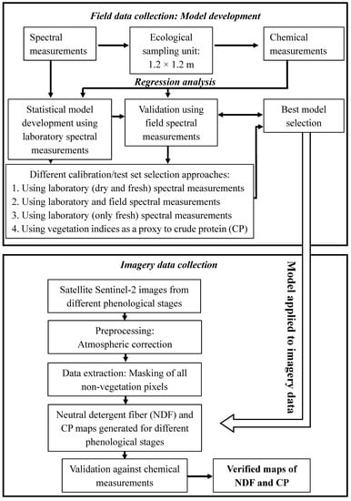
Figure 1.
Flow chart of the study’s general methodology.
To track the seasonal variability of habitat quality, we followed the ecological approach by means of sampling methods and imagery temporal analyses [24,41]. Sampling methods are clarified in Section 2.2. Temporal estimation relied on the analyses of eight Sentinel-2 images that were taken at different phenological stages. Seven images were used for spatial prediction of CP and NDF using the best-accuracy models, and one image was used for validation of results. All Sentinel-2 images were atmospherically corrected. We used reflectance data as well as reflectance transformed to FD and KM units, and slopes between the various spectral channels were calculated. All non-vegetation pixels were masked. Finally, CP and NDF maps for each model (reflectance, FD, KM, and slopes) were generated for all Sentinel-2 images. Ten samples and their corresponding chemical measurements were used to validate spatial mapping results. Only best-accuracy predictions are reported here. Below, in Section 2.1, Section 2.2, Section 2.3, Section 2.4, Section 2.5, Section 2.6, Section 2.7, Section 2.8 and Section 2.9, various stages of our analyses are described in more detail.
2.1. Study Areas
Two pasture areas were selected for this study, each with different climatic conditions and soil qualities: Ramat Menashe and the Patish Basin (Figure 2a,b). Ramat Menashe is located in the southern Carmel hills (32°34′N; 35°6′E), with an average height of 400 m above sea level (ASL). The climate is mostly Mediterranean, with rainfall from November to April and a cattle-grazing period from mid-February to mid-May. The long-term annual rainfall average is 580 mm, dropping to around 360 mm in dry years and rising to 800 mm in rainy years [42]. The soil is shallow dark Rendzina (Mollisol according to USDA soil taxonomy), 10–25 cm in depth, on Eocenic bedrock. The composition of the vegetation is 80–90% annuals, and 10–20% perennials and stones. A high diversity of annual vegetation (about 9% legumes, 38% grasses, and 53% forbs) covers the area during the growth season in the spring. The dominant perennials (shrubs) in this area are Echinops polyceras and Foeniculum vulgare Mill., with Sarcopoterium spinosum on the ungrazed northern slopes. The grazing period of the cattle is 29 grazing days per hectare during the green season, and 52 days during the dry season [43]. Ramat Menashe is a long-term ecological research (LTER) site; three study plots (GL1–GL3, Figure 2c) and one control plot (GL4) were set.
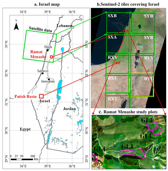
Figure 2.
(a) Map of Israel. (b) Sentinel-2 tiles covering Israel, with the study areas Ramat Menashe and Patish Basin indicated with red rectangles. The northern site was used to collect field measurements for model validation, and the southern site was used to collect vegetation samples for laboratory analysis for the purposes to developing models. (c) The four study plots at Ramat Menashe (borders in magenta) shown on a Sentinel-2 image.
The Patish Basin (31°22′N, 34°40′E) is located in the northern part of Israel’s Negev desert and it spans a hilly area of 230 km2, with an average height of 150 m ASL. The climate is semi-arid, with rainfall from November to April, and a long-term annual rainfall average of 200–300 mm [42]. The grazing season is from mid-February to mid-May, when the annuals are at peak growth; this growth tails off in mid-spring (March–May) when the annuals are subjected to dry conditions [44]. The soil is Loess with a sandy loam texture (Calcixerollic, Xerochrepts according to USA classification), 1 m in depth, on Eocene bedrock [45]. The main land use is natural pasture, moderately grazed by Bedouin-owned herds of Awassi sheep. The dominant perennial species in the research area are the shrubs Atractylis serratuloides (Asteraceae), Noaea mucronata (Chenopodiaceae), and Thymelaea hirsuta (Thymelaeaceae); the geophyte Asphodelus ramosus (Liliaceae); and the Tamarix negevensis tree. The main annual species are Reboudia pinnata (Brassicaceae), Avena sativa (Poaceae), Stipa capensis (Poaceae), Hordeum glaucum (Poaceae), Bromus scoparius, Crepis sancta, Chrysanthemum coronarium, Scolymus maculatus, Senecio flavus, Atriplex spp, and Centaurea iberica [46]. The vegetation samples were collected from three study sites in the Patish Basin: the Gilat Research Center (31°20′36.43′′N, 34°40′20.04′′E) and Shaked Park (31°16′12′′N, 34°39′2.75′′E), both long-term ecological research (LTER) sites, and a path along the herd grazing route [6].
2.2. Sample Site Identification: Ecological Approach
In order to properly describe the spatial pattern of habitat quality and its extent within the study areas, a benchmark survey was conducted. The latter determined whether the pattern or process was on a local, regional, or global scale. We used the ecological typical benchmark habitat method described in [47,48,49]. Briefly, long transects were set up at each of the two study plots in Ramat Menashe (GL1 and GL2, Figure 2c). Four parcels, each of 1.2 m2 (Figure 3C.1), were established along each transect, 10 m distance from each other. One parcel each, in GL3 and GL4 also were established. In situ spectral measurements and laboratory chemical analyses were conducted on vegetation samples from a total of 10 of these parcels.
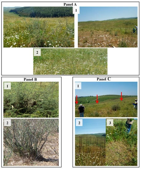
Figure 3.
Views of the study area, representative vegetation samples, and sampling approach. Panel A. 1. Views of the study area; 2. Diversity of annual cereals. Panel B. The dominant perennials: 1. Echinops polyceras; 2. Foeniculum vulgare mill. Panel C. 1. Ecological approach: cross-section sampling; 2. Fenced plot as control with no grazing; 3. Plot after biomass harvesting.
2.3. Chemical Analyses: Reference Measurements
We used CP and NDF as indicators of pasture quality. Immediately after the spectral measurements, all vegetation samples were oven-dried for 72 h at 60 °C, ground to pass through a 1-mm sieve and 25 g each of sample subjected to chemical analysis for CP and NDF [6]. The chemical analysis for CP was performed using the automated Kjeldahl method, and for NDF, according to Goering and Van Soest [15,50]. CP was determined by acid digestion [51]. NDF was measured using a detergent that solubilizes the proteins and sodium sulfite, and that helps to remove some of the nitrogenous matter and similarly to Van Soest [52]. NDF content was determined as: {([crucible weight + fiber] − crucible weight w/o fiber)/(sample weight × lab, dm as decimal)} × 100 [6,52]. Log-transformed values of CP and NDF were also calculated, to obtain a normal distribution of reference values for partial least squares (PLS) analysis.
2.4. Field Measurements
2.4.1. Sample Collection
Two sets, field in-situ and laboratory measurements, were conducted using the Analytical Spectral Devices (ASD) Fieldspec-Pro JR Spectroradiometer [53], at the Ramat Menashe and Patish Basin sites.
At the Ramat Menashe site, field measurements were conducted on 20 April 2017 (between 10:00–14:00), a day before Sentinel-2 data acquisition. Four enclosures of 1.2 m2 each were defined within each of the plots GL1–GL2, and two additional were defined in GL3 and in GL4 respectively. After spectral measurements at each of the enclosures, the vegetation was cut (Figure 3C.3) and collected into paper bags for chemical analysis. A total of 10 fresh vegetation samples were collected. All spectral measurements were conducted under clear-sky conditions.
At the Patish Basin, 36 fresh vegetation samples were collected from the Gilat Research Center and Shaked Park sites on 12 March 2013, and 16 partially fresh and dry samples were collected along the herd grazing path on 5 November 2012 [6]. All parts of the vegetation sample (leaves, stems, and grains) were cut off and were kept in paper bags for spectral measurements at laboratory condition and chemical analysis. A total of 47 out of 52 vegetation samples were used in developing regression models.
2.4.2. Spectral Measurements
The ASD measures spectra in 2151 bands across 350–2500 nm. To obtain reflectance values, the spectra was presented against a white Halon panel reference [54]. At Ramat Menashe, spectral measurements were conducted in ten parcels of 1.2 m2 each; in each parcel, a total of five spectral measurements were taken—one in each of the four corners, and one in the middle (Figure 3C.2). Then, the measurements were averaged. A bare fiber was set up to measure from the nadir position at a height of 50 cm above the vegetation canopy, with instantaneous field of view (IFOV) of 23 cm. The totals of 10 (averaged) spectra obtained at Ramat Menashe were used for validation of regression models. At the Patish Basin, the reflectance spectra of samples were measured under laboratory conditions, via direct contact of the probe to the vegetation sample. The spectral measurements of vegetation samples were conducted at the sampling day. The total of 47 spectra obtained was used to develop regression models, as described below. After spectral measurements, all vegetation samples were subjected to laboratory chemical analysis for CP and NDF.
2.4.3. Data Pre-Processing
All field and laboratory spectral measurements were spectrally resampled to match the configuration of Sentinel-2 data, for 12 out of the 13 bands in the VIS-NIR-SWIR spectral region. Band 10 (1373 nm) was not included in the resampled data because the atmospheric correction results also omitted this channel (see Section 2.5.2 below). The spectral resampling was carried out using the “spectral resampling” procedure provided in the ENVI software (version 5.2) [55]. It requires spectral channels central wavelength as input, then the algorithm assumes critical sampling range, and uses a Gaussian model with a FWHM (Full Width at Half Maximum) that is equal to the band spectral range.
Next, different pre-treatments techniques were applied on both field and laboratory spectral measurements, in order to improve the predictive ability of the constructed model [40]. Specifically, the reflectance data was transformed to First Derivative (FD), and to Kubelka–Munk (KM) units, and slopes between pairs of bands were calculated. FD transformation used the Savitzky–Golay [40,56] method for computing first- or higher-order derivatives, with a smoothing filter that reduces instrumental noise and that determines how many adjacent wavelengths will be used to estimate the polynomial approximation for derivation [40]. A polynomial order of one was used. The KM theory assumes a linear relationship between spectral intensity and sample concentration [57], and is calculated as (1−R)2/2R, where R is the reflectance [58]. The KM transform of the measured spectra is approximately proportional to the absorption coefficient, and hence, to the concentration. Generally, the KM spectral curves reduce high-frequency noise without degrading the shape of the original spectra [56].
Slopes between bands were calculated after the reflectance data was transformed to continuum removal (CR) units. The commonly used CR technique [18,22,55,59,60] normalizes the reflectance spectra to a baseline, thus enhancing spectral differences and enabling the identification of individual absorption features. Slopes were calculated using the following equation: slope = ((y2 − y1)/(x2 − x1)), where the x-axis represents wavelength, and the y-axis represents CR values [7]. To find the best slopes, all possible pairs of channels were examined.
2.5. Imagery Data: Sentinel-2
2.5.1. Data Collection
Sentinel-2 produces spatial and temporal images that cover the VIS-NIR-SWIR spectral region. It carries a multi-spectral instrument (MSI) with 13 spectral channels, covering a range of wavelengths from 400 to 2300 nm with spatial resolutions of 10 m (496 nm, 560 nm, 665 nm, and 835 nm), 20 m (705 nm, 740 nm, 783 nm, 865 nm, 1610 nm, and 2202 nm), and 60 m (443 nm, 945 nm, and 1373 nm). The temporal resolution of a satellite is 10 days [61]. To obtain a spatial representation of CP and NDF levels, and a temporal representation along the growing period using Sentinel-2, cloud-free images of the Ramat Menashe area (Figure 2a,b) were downloaded from the archives of the USGS Earth Explorer website [62]. A total of six Sentinel-2 images were used for CP and NDF mapping along the growing season (28 December 2015, 17 January 2016, 16 February 2016, 7 March 2016, 16 April 2016, and 20 February 2017); one image was used for the dry season (15 July 2016); and one was used for validation (21 April 2017). We used a Level-1C product, which comprises geo-coded, top-of-atmosphere reflectance, with a sub-pixel multi-spectral registration [63].
2.5.2. Sentinel-2 Image Pre-Processing
The Sen2Cor atmospheric correction processor was used to retrieve surface reflectance [64]. The atmospheric correction processing include: (1) bottom of the atmosphere (BOA) reflectance, (2) Cirrus Correction algorithm that uses the Sentinel channels 10 and 3 to identify cirrus clouds and cloud shadows respectively. We used rural (continental) aerosol type with mid-latitude summer and of 331 Dobson Units ozone concentration [65]. The Sen2Cor output product format is equivalent to the Level-1C user product: JPEG 2000 images with three different spatial resolutions—10, 20, and 60 m—without the water absorption band (channel 10:1373 nm). Next, the resolutions of 10 and 60 m were resampled to 20 m, using the “special resampling” procedure provided in the ENVI software (version 5.2) [55]. The final image contains 12 channels with a 20 m spatial resolution.
The Normalized Difference Vegetative Index (NDVI) was calculated for all Sentinel-2 images. NDVI, based on the red and near-infrared (NIR) reflectance ratio, is used as a temporal indicator of the vegetation cover, and is calculated by: NDVI = (NIR − Red)/(NIR + Red)), where NIR and Red are the reflectances of the corresponding spectral channels [66]. A threshold of NDVI < 0.35 was used as a condition for masking non-vegetation pixels for all images except April 21, 2017 (the latter was used for validation). Generally, the growth peak is at the end of February–March. In April, some vegetation had already been consumed by herds. Hence, for this image, the masking threshold was adjusted to the minimal NDVI value obtained from the field measurements collected at Ramat Menashe on 20 April 2017 (the previous day), and was set at NDVI < 0.25. Finally, we applied the above-mentioned pre-treatments (FD, KM, and slopes) to the spectral domain for all Sentinel-2 images.
2.6. Meteorological Data
Monthly precipitation and air temperature measurements from ground monitoring stations of the Israel Meteorological Service were obtained for 2016 and 2017 [42].
2.7. Statistical Analysis: Regression Models
Calibration equations were created by using PLS regression performed on the reflectance, FD, KM, and slope data, following resampling to the Sentinel-2 configuration, for each chemical reference (CP and NDF) separately:
where Y is the chemically measured CP or NDF content of a vegetation sample; A1–An are empirical coefficients at specific wavelengths/slopes; and X is a spectral reflectance/FD/KM value at a specific wavelength, or a slope of the spectra in a specific range. We used a leave-one-out cross-calibration approach.
To estimate the accuracy of our models, we constructed different calibration, validation/test sets, and used random as well as supervised samples selection (see Section 2.8). The statistical accuracies of all models were assessed by the root mean square error of prediction (RMSEP), or by the root mean square error of cross validation (RMSECV) [67]:
where Ym is chemically measured, and Yp is the predicted value of a sample using spectral measurement, and n is the number of samples used in the calibration stage. The best model was selected based on the lowest RMSEP (%) and the highest coefficient of determination (R2). All data analyses were performed using SAS software (version 9.4). We also compared statistical parameters between both the calibration and validation data sets, to assure that they provided a similar range of values. In other words, calibration sets are representative of the validation/test sets [67].
An additional supporting parameter for choosing the best prediction model is the index of agreement [68,69]. The index is a measure of accuracy, and it is aimed at evaluating the model performance:
where Oi is a chemically measured value, Pi is a predicted value, and Ō is the average of the measured samples. The index varies from 0 to 1, where higher values indicating better agreement with the measured data, and lower values indicate models that are less or not accurate.
2.8. Model Development: Selection of Calibration/Test Sample Sets
As we noted previously, all spectral measurements were resampled to Sentinel-2 configuration. Thereafter, Partial Least Squares (PLS) regression analysis was run on the laboratory (fresh and dry vegetation samples) and field (fresh) measurements, using different configurations. Five different options of choosing calibration/validation data sets were considered and tested.
1. Leave-one-out cross-calibration models were run on reflectance measurements and transformed reflectance (e.g., using different pre-treatments techniques: FD, KM, and slopes), to develop the best prediction model for CP and NDF. Each data set consisted of 47 laboratory spectral measurements, and 10 from the field were used for validation. The best selected model used a total of 43 out of 47 samples. Additional models were constructed (e.g., options 2–4 below). This need was mainly governed by the relatively small number of samples available in our study.
2. Random selection. Five different randomly selected calibration data sets were constructed. Each set consisted of the above-mentioned 43 samples: 33 for calibration, and 10 samples for validation. In addition, we used an external test set of seven (field) samples.
3. Laboratory and field samples in a model. An important question examined in this study is whether including the field (fresh) measurements from Ramat Menashe site with the laboratory (fresh and dry samples) measurements improved the model accuracy. To that end, we used 43 laboratory measurements and six from the field measurements (four from GL1 and two from GL3, GL4), in a total of 49 vegetation samples. The vegetation samples from GL2 parcel were not included in the calibration models, and used for validation. Then, five randomly chosen datasets were constructed. Each dataset included 39 samples for calibration, and 10 samples for testing.
4. Only fresh samples in a model. Here, we examined whether reducing dry samples impacts on the model accuracy. To that end, we ran leave-one-out PLS models on 36 fresh samples (out of 43, of the selected best model).
5. Using three vegetation indices as a proxy for CP and NDF estimation. A correlation between CP/NDF contents and the aboveground biomass of vegetation, using remotely sensing data has already been reported [70,71,72]. If so, this would necessitate the development of spectral models for CP and NDF estimation. To investigate this point, we used NDVI [66], SAVI (Soil-adjusted Vegetation Index) [73], and WDRVI (Wide Dynamic Range Vegetation Index) [70]. Similar to our previous sample selection, the same 43 vegetation samples were used, and leave-one-out statistical approach was applied.
2.9. Model Validation
A total of 10 spectra were received and used to validate the accuracy of CP and NDF predictions (e.g., eight in GL1 and GL2, and two in GL3 and GL4). The best model was selected based on the statistical parameters used in our study, and reference chemical measurements. To this end, the estimated CP and NDF generated from the model using Sentinel-2 image from 21 April 2017 were compared to the CP and NDF data obtained from the vegetation samples collected on 20 April 2017.
3. Results
3.1. Chemical References: CP and NDF
The range of CP and NDF data used to develop models was wider than the range of data used for the validation of the selected best model. For the model development data (47 samples), the average, STD, and range of CP values were 9.6%, 3.9%, and 3–17.2% respectively; for the NDF values, the average, STD, and range were 52.5%, 12%, and 27–71%. For the validation sample data (10 samples) the average, STD, and range of the CP values were 7.5%, 0.95%, and 5.9–9.2%; for the NDF values, the average, STD, and range were 64.9%, 4.85%, and 57–73%.
For the Patish Basin field measurements, the determination coefficient between the measured CP and NDF was R2 = −0.65 (n = 47), whereas for the Ramat Menashe field measurements, R2 = −0.47 (n = 10).
3.2. Spectral Analysis
Figure 4 presents the reflectance and FD spectra, from the laboratory measurements, of four fresh vegetation samples and one dry vegetation sample with different percentages of CP and NDF. The results demonstrate changes in reflectance/FD across the Sentinel-2 bands as a function of different CP and NDF contents. For example, increasing the reflectance at 740 nm, 783 nm, 865 nm, and 945 nm correlated with increasing CP and decreasing NDF content, whereas decreasing the reflectance at 560 nm, 665 nm, 1610 nm, and 2202 nm correlated with increasing CP and decreasing NDF content.
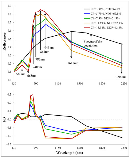
Figure 4.
Reflectance (upper) and First Derivative (FD) (lower) spectra of five vegetation samples (laboratory data set) with different percentages of CP and NDF. Note the variability in reflectance and FD across the spectral bands, with associated changes in CP and NDF concentration. Specifically, as reflectance increases at 740 nm, 783 nm, 865 nm, and 945 nm, CP values rise and NDF values fall; and as reflectance decreases at 560nm, 665nm, 1610 nm, and 2202 nm, CP values fall and NDF values rise.
3.3. PLS Analysis of Different Selection Models
A score plot of samples from the PLS model for CP is shown in Figure A1. To assess CP and NDF, the first four LV (latent variable) components in the PLS model explained 98% of the X variance (reflectance), and 85% (for CP) and 73% (for NDF) of the Y variance (chemical components). This indicated that most of the spectral variation is related to the CP and NDF. Furthermore, there was a good correspondence between spectral reflectance and chemical constituents (CP and NDF), as explained by the first LV components. The first LV component reflects the quantitative change in CP% content measured in the samples whereas the second LV component exhibits the change in water content that impacts spectral reflectance of all surfaces. Specifically, the CP content increases from left to right along the axes, and water content increases from top to bottom (Figure A1) [6].
Table 1 summarizes the PLS regression analyses for the FD, reflectance, slope, and KM models. In general, the highest R2 for predicted CP is produced by the FD model (0.764) and for predicted NDF by the slope and reflectance models (0.778 and 0.775, respectively). Note that all models were found to be significant (p < 0.05). The index of agreement values of the different models are good and varied between 0.71–0.78 for CP and between 0.73–0.78 for NDF (Table 1). PLS regression analyses, when run only on fresh vegetation samples (Table 1) was found to be significant, with an R2 of 0.592 for CP, and 0.698 for NDF correspondingly, and the index of agreement was 0.64 for CP and 0.7 for NDF.

Table 1.
Partial least-squares (PLS) regression model results for the reflectance and slope methods, and for various data pre-processing techniques for the estimation of CP and NDF in fresh vegetation.
The selected best prediction models for CP (called S2_CP_RI: Sentinel-2 Crude Protein Reflectance Index) and NDF (called S2_NDF_RI: Sentinel-2 Neutral Detergent Fiber Reflectance Index) were reflectance-based. The Sentinel-2-based formula generated by these models is presented in Table 2.
Table 2.
Prediction models for CP and NDF, using the reflectance-based method.
Figure 5 presents the measured vs. predicted values of CP and NDF at Ramat Menashe (field measurements vs. results from the selected best model, based on reflectance spectra). The R2 for CP is 0.67 (seven out of 10 vegetation samples), and for NDF, 0.75 (nine out of 10 samples). Although our results show relatively high correspondence between measured vs. predicted CP and NDF values, it should be noted that the samples represent only a relatively small dynamic range of reference values. This is especially true for CP. Thus, even extremely small differences between the modeled and actual values strongly influence RMSEP in a positive direction. However, these results also highlight a certain bias (e.g., slope) of our model when it is used on the external test set samples. This bias is due to several reasons: (1) a small number of samples; (2) four samples have similar %CP values, resulting in a spurious scatter.
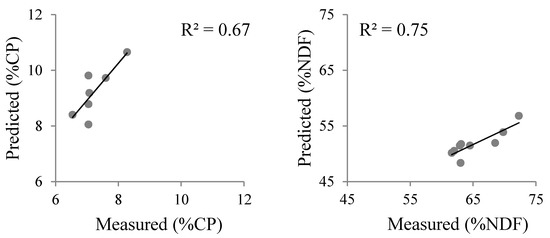
Figure 5.
Measured vs. predicted values of chemical data, using the selected best model applied on field measurements. Note a larger bias in the estimation of NDF.
In light of the results presented in Figure 5, several additional steps were further implemented to verify the accuracy of our models: (1) Five additional randomly selected data sets were constructed (Table 3); (2) models were examined using a test image, and estimated values were compared to the laboratory measurements.
Table 3.
Statistical parameters obtained for different randomly selected data sets. Forty-three samples of the selected reflectance-based model were used.
Table 3 summarizes the PLS regression analyses results for randomly selected calibration samples in five different data sets. As can be seen, all models are significant, with a relatively good and comparable R2 and index of agreement being obtained for all data sets.
Another important question relates to whether the addition of field measurements to the laboratory measurements improves the model results. In Table 4, we estimated the accuracy of a joint data set. Applying these models on the Sentinel-2 image from 21 April 2017 resulted in a good agreement with the field measurements. Similarly to our results in Table 3, all models were significant, with relatively good R2 and low RMSEC (%) (R2 ranges of between 0.69–0.72 for CP and 0.63–0.71 for NDF).
Table 4.
Statistical parameters obtained for different randomly selected data sets, using the laboratory and field measurements.
Figure 6 presents the distribution, average, and STD of CP and NDF for field measurements from Ramat Menashe, shown against the corresponding pixel values of the region of interest (ROI) that bounds the sampling location in each study plot (GL1–GL4). As can be seen, when the model (Table 4) was run on the GL2 parcel (which did not participate in the model construction), it provided a comparable degree of accuracy (average CP values for GL2 chemically measured = 7.69% vs. estimated values ranging between 7.3 to 7.45% and for NDF 64.62% vs. 64.38–65.1%, respectively. Note the improvement in NDF estimation using the joint data set (64.38-65.1%), compared to our best model (56.59%,).
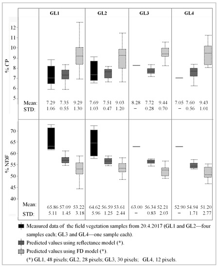
Figure 6.
Distribution of the crude protein (%CP) and neutral detergent fiber (%NDF) contents obtained from field measurements (from 20 April 2017), and of the predicted values obtained by applying reflectance and FD models on a Sentinel-2 reflectance image (from 21 April 2017), for each plot.
The results shown in Figure 6 were received after implementing the reflectance and FD models on Sentinel-2 data from 21 April 2017. It can be seen that the average, STD, and range values of the reflectance model were closer to the field measurements than the FD model.
In Table 5, we compare between reflectance-based models (the best selected) and vegetation indices-based models. As can be seen, the reflectance model provides much better accuracy than indices-based models. Although for CP, when the indices-based model was significant, poor R2 was achieved (0.35–0.37). Note that NDF estimation models were not found to be significant (p > 0.12), with R2 ≤ 0.06.
Table 5.
Partial least-squares (PLS) regression results for reflectance-based (the best selected) and vegetation indices-based models.
3.4. Mapping CP and NDF Contents using Sentinel-2 Images
Figure 7 presents the estimated spatial variability map of the CP and NDF contents, using the reflectance models S2_CP_RI and S2_NDF_RI, during different phenological cycles: at the beginning of the winter season (28 December 2015); during the vegetation growth period (17 January 2016 and 16 February 2016); at the peak of vegetation growth (7 March 2016); during the grazing period (16 April 2016); and during the summer season (15 July 2016). For each period, an inverse relation between CP and NDF was evident: CP increased as NDF declined. Note that with the coming of March, when vegetation growth reached its maximum (RGB image used as reference, Figure 7), the number of pixels that met the NDVI criteria (NDVI ≥ 0.35) increased; this number then declined in April and dropped significantly in summer. In addition, the CP and NDF maps show their values increasing and decreasing (respectively) during the winter season until a peak was reached on 7 March 2016, which was then followed by a fall in CP and a rise in NDF, as measured on April 16, 2016. In the summer (15 July 2016), the amount of vegetation declined significantly, lowering the total CP content available to herds. Specifically, the CP averages for the study area (not including pixels with NDVI < 0.35) were 7.2%, 7.5%, 8.3%, 9.6%, 8.5%, and 7.6%; the NDF averages were 59.2%, 9%, 57.4%, 54.1%, 55.8%, and 57.3% (for 28 December 2015; 17 January 2016; 16 February 2016; 7 March 2016; 16 April 2016; and 15 July 2016, respectively).
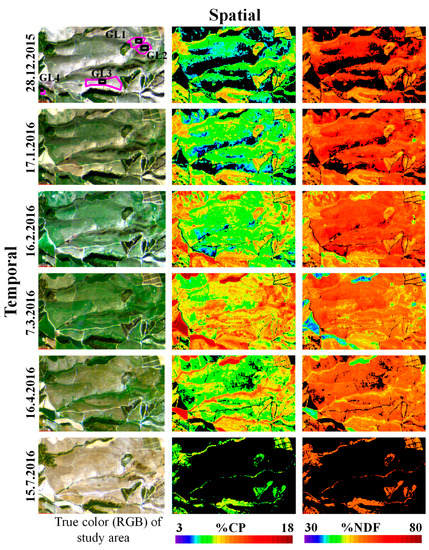
Figure 7.
Temporal changes in CP (middle) and NDF (right) contents of the study area. The black pixels are masked pixels (NDVI < 0.35). The magenta-bounded areas on the 28 December 2015 image are the study plots (GL1–GL4), and the black rectangles indicate the sampling locations in each plot. Note also that the RGB version (left) shows variability in vegetation color/properties.
The left panel shows the estimated spatial CP maps obtained using the reflectance (b) and the FD (c) models, while the right panel (d, e) shows the frequency distribution of the estimated CP values, for the same pixels produced by each model. Note that the reflectance model was found to be slightly less accurate than FD (index of agreement = 0.72 vs. 0.71 and R2 = 0.76 vs. 0.71 (Table 1), consequently). The maps were generated for a Sentinel-2 image from 21 April 2017, and they highlight the differences between the two models. In the reflectance-based map (b), the CP values were higher in the dense vegetative areas, while the FD-based map (c) was a noisy image, with a salt-and-pepper appearance that made the interpretation of results difficult. In addition, the frequency distribution of CP values was overestimated in the FD-based map, with an average value of around 9.5% (e), comparing to 8% using the reflectance-based model (d), and validatory vegetation samples (7.5%). This result suggests that the FD model, while returning a higher R2 and lower RMSEP, exhibits overfitting, and it is less reliable for CP estimation. Furthermore, as also evident from the wheat field area (shown with a black ellipse on Figure 8a), the reflectance model (Figure 8b) also provides a much easier interpretation of CP values within agricultural plots than the FD model (Figure 8c).
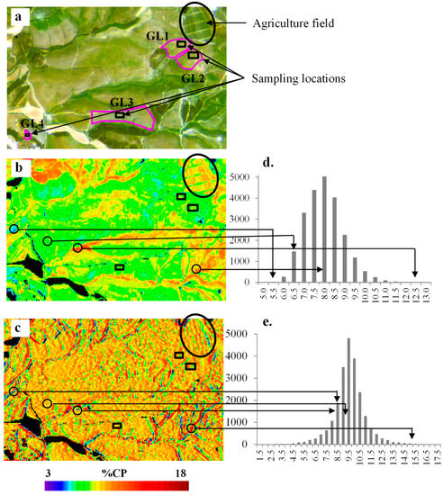
Figure 8.
Visual and quantitative differences between two models applied to a Sentinel-2 image: the reflectance model (selected best model) and the first derivative (FD) model. (a) True color of the study area. The magenta-bounded areas are the study plots (GL1–GL4), and the black rectangles indicate the sampling locations in each plot. (b) Estimated CP map generated from the reflectance model (c). Estimated CP map generated from the FD model. Note the increased noise level in (c), (d)/(e) Frequency distribution of the estimated CP values for all pixels in the study area, using the reflectance-based model (d) and the FD-based model (e). The black ellipse shows a wheat field as an example of CP variability within an agricultural plot. Note that the reflectance model makes the visual interpretation of CP values much easier than does the FD model.
3.5. The Influence of the Meteorological Conditions on the Patterns of CP and NDF
Figure 9 shows comparisons between the two winter seasons in 2016 and 2017: Panel A compares the meteorological parameters (rainfall and temperature); Panel B shows the estimated spatial CP and NDF per pixel, obtained using the reflectance model; Panel C displays the frequency distributions of the estimated per-pixel CP values shown in Panel B (pixels with NDVI < 0.35 were excluded). The total amount of precipitation was higher in 2017 than in 2016 (466 mm vs. 334 mm), with a substantial difference between two winters observed in the three months of December through February. Total precipitation of 289 mm was measured in December 2015–February 2016, with a maximum of 148 mm in January and 426 mm in December 2016–February 2017, with the maximum of 288 mm in December 2017 (Figure 9A). In addition, the air and near-ground temperatures were higher in 2016 than 2017, with differences between two seasons ranging from 0.2–2.4% and 0.7–4.1% (for air and near-ground temperatures, respectively) (Figure 9A). In other words, winter 2017 was colder and wetter than winter 2016, which would be expected to result in greater vegetation growth. This difference seems to impact the CP contents that tend to be higher in February 2017 relative to 2016 (Figure 9B). Furthermore, the CP distribution diagram reveals a shift toward higher %CP values in 2017 (Figure 9C). The NDF pattern was found to be reversed compared to CP: lower in February 2017 compared to February 2016.
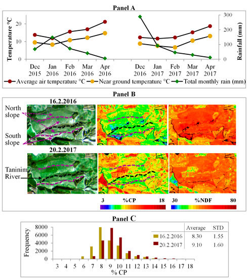
Figure 9.
Comparisons between two winter seasons in 2016 and 2017 of: monthly rainfall and temperature (Panel A); estimated spatial CP and NDF maps using the reflectance model (Panel B); and frequency distributions of the per-pixel CP values (Panel C) in the maps shown in Panel B.
4. Discussion
For the majority of our models, the PLS analysis returned a relatively low RMSEP and a high index of agreement (ranging from 0.71 to 0.78) and a relatively high R2 (0.71–0.778) (Table 1). This was despite the fact that the samples used to develop the models were collected from the Patish Basin site, which is a semi-arid climate area, whereas the models were then applied and validated in the mostly Mediterranean climate of the Ramat Menashe site. The two sites are located at a distance of 145 km from each other, and they have similar vegetation properties (as evident in Figure 10). Indeed, Figure 3 shows that annual species in Ramat Menashe from the Gramineae (Poaceae) family—such as Stipa capensis, Hordeum glaucum, and Bromus scoparius—are also part of the annual ecological community in the Patish Basin (Figure 10) [46,74]. Based on our results, the distance between the sites does not have a significant impact on the accuracy of our models for predicting the CP and NDF contents.
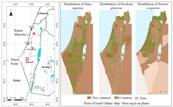
Figure 10.
An example of the spatial distribution of annual species in Israel.
As mentioned above, the models that were selected for spatial mapping are reflectance-based: S2_CP_RI for CP and S2_NDF_RI for NDF (Table 2). Furthermore, our best selected models were developed using a mixed-sample dataset (fresh and dry vegetation samples). When the dry samples were removed, the R2 was lower and RMSEP was larger comparing to models that combined both the fresh and dry samples (R2 = 0.592 for CP, 0.698 for NDF, vs. 0.711 for CP, 0.775 for NDF, Table 1). These results are important, because along the growth period, dry vegetation can be found in the pasture area. This “mixed” vegetation selection was previously reported [6]. In that study, different dry-to-fresh ratios were used, and a good R2 was found for most of them. For the current study, we used a ratio of 17% dry to 83% fresh. As can be seen in Figure 3, the vegetation in the study areas is mostly fresh; however, there are also different levels of dry vegetation.
Our PLS analysis includes different wavelength bands that were selected to generate a model with the most accurate estimation of CP and NDF contents (Table 1). Wavelengths at 560 nm, 665 nm, 865 nm, and 2202 nm were found to be the most important in our analyses. Note that in all models, the 865 nm band and 2202 nm band were found to be important (Table 1). The estimation of CP and NDF contents in plants using the VIS-NIR spectral range has been reported [29,75,76,77,78,79,80,81]. Similar to our results, Starks et al. [26] reported that narrow wavebands (e.g., reflectance centered at 485 nm, 605 nm, 725 nm, 755 nm, 765 nm, 865 nm, and 915 nm (±5 nm)) had greater R2 with CP and NDF availability. The findings of Kawamura et al. [78] indicate that CP and NDF can be estimated with wavebands in the VIS-NIR region by using ground-based canopy reflectance: CP with 700–705 nm, 725 nm, 760 nm, and 775 nm, and NDF with 720–745 nm, 700 nm, 715 nm, and 760 nm.
It is interesting to note that many studies have reported that foliar nutrient concentrations across the VIS-NIR spectral range are related to protein [22,78,81,82,83,84,85,86]. Nitrogen is an essential element in the life-activity of vegetation, having an important function in the biosynthesis of proteins, nucleic acid, chlorophyll, and enzymes, and playing a crucial role in vegetation photosynthesis [87]. For example, Clifton et al. [82] found that nitrogen analyses confirmed that reflectance measurements in red (650–670 nm) and NIR (830–850 nm) were accurate predictors of green CP density for a variety of grass swards. Indeed, the Kjeldahl method measures CP concentrations by determining nitrogen, with a factor of 6.25 being used for the conversion of N into CP [88]. Moreover, strong predictive relationships between spectral reflectance in VIS-NIR region and canopy foliar N concentration were found by using hyperspectral data (from the Hyperion satellite, and from AVIRIS airborne and lab/field spectrometers) [79,80,87,89,90,91].
The SWIR region is also widely used for CP and NDF estimation in forage [6,7,13,29,76,78,92,93,94,95,96,97,98]. Our results are in agreement with other studies that have also reported the importance of the SWIR region, and specifically for the wavelengths of 2202 nm (CP in rapeseed, R2 = 0.98 [99] and 2204 nm (NDF in forage, R2 = 0.97 [16]. The SWIR spectral range contains information about the major X–H chemical bonds, due to vibrations arising from the stretching and bending of H bonds associated with C, O, and N. For examples, the protein-associated N–H and C–H bonds absorb at 2060 nm, 2130 nm, and 2180 nm (N–H) and at 2240 nm (C–H) [100,101,102,103,104].
The spatial mapping of CP and NDF contents, shown in Figure 7, revealed an inverse relationship between the two components during different phenological cycles. These results were also supported by the in situ field measurements from the Ramat Menashe (R2 = −0.65, p < 0.05) and Patish Basin (R2 = −0.47, p < 0.05) sites. Other studies have also found this relationship by using laboratory measurements [105] or NIRS analysis [29,76,106]. For example, Pullanagari et al. [29] found that the coefficient of determination between CP and NDF was R2 = −0.804 (p < 0.001). As can also be seen in Figure 7, the CP and NDF maps revealed (respectively) increasing and decreasing trends over the winter season, reaching maximum/minimum values on 7 March 2016, followed in turn by a fall in CP and a rise in NDF (Figure 7). It is interesting to note that this increase/decrease of CP/NDF is accompanied by an increase in NDVI until 7 March 2016, followed by a substantial decrease toward July. Specifically, the averaged NDVI for the Ramat Menashe site was 0.43, 0.54, 0.63, 0.69, 0.52, and 0.19 for 28 December 2015, 17 January 2016, 16 February 2016, 7 March 2016, 16 April 2016, and 15 July 2017, respectively.
The true color of the time series of Sentinel-2 images (Figure 7) indicates an increase in biomass up to a peak on 7 March 2016, followed by a substantial decline to a low in July. Thus, CP and NDF maps produced using the reflectance-based model can indicate the relationship between NDVI, biomass, and protein content, as shown in Figure 7. A correlation between the CP content and the aboveground biomass of vegetation, using remote sensing data, was previously reported in the literature [70,71,72,107,108,109,110,111,112,113]. In other study, Filella et al. [109] found that in the Mediterranean ecosystem, NDVI was sensitive not only to biomass and phenology changes, but also to protein content. In this regard, a reader may assume that NDVI can be used as a good proxy for CP/NDF contents, and using reflectance-based or any other models is useless. However, as our results indicate, NDVI, SAVI, WDRVI provide poor accuracy in CP and NDF estimations (Table 5). Furthermore, the estimation of NDF is only possible by using a reflectance-based model.
For Mediterranean ecosystems, rainfall seasonality (the length of the growing season and the timing of the rainfall) and air temperature are important factors that influence the variability of the vegetation during the growth season [106,114]. Our findings suggest that precipitation and temperature might affect CP and NDF contents on spatial and temporal scales. As can be seen in Figure 9A, the monthly precipitation and the precipitation patterns between December and April in two subsequent years (2016 and 2017) were different. The winter of 2017 brought more rain overall than the winter of 2016, with a significantly larger amount of precipitation falling at the beginning of the growth season. The total rainfall between December and April was 335 mm in 2016 and 466 mm in 2017, with respective maximum monthly figures of 148 mm (in January 2016) and 288 mm (in December 2016). On the other hand, the monthly average air and near-ground temperatures were higher in 2016 than in 2017 (Figure 9A). The lower near-ground temperatures in 2017 would have resulted in a lower evaporation of water in the soil; together, higher precipitation and lower temperatures lead to greener vegetation for a longer period of time [115]. Green vegetation tissues may have a high nitrogen content (protein) and low NDF content [116]. Accordingly, it is interesting to note the differences between the CP maps for the same period in each of these two years, from 16 February 2016 and 20 February 2017 (Figure 9B). As can be seen, the CP content was significantly higher in 2017 than in 2016. Also, the CP distribution diagram (Figure 9C) shows a shift toward higher CP values in 2017. The equivalent NDF map (Figure 9B) shows an inverse pattern to the CP map, and thus, it also matches the rainfall and temperature patterns, with significantly higher NDF content in 2016, than in 2017.
It is not only precipitation and temperature that affect the total CP and NDF content. Topography also has a pronounced influence, with the CP content on northern hillslopes being found to be higher than on southern hillslopes. Interestingly, this difference was apparent in February 2016, but not in February 2017, as seen in Figure 9B. In this regard, we may speculate that the higher precipitation between December 2016 and February 2017, compared to the same period in the previous year served to obscure the differences caused by hillslope aspects. Differences between hillslope aspects stem from differences in radiation intensity: at 30°N latitude, the radiation is more intense on the southern slopes than on the northern slopes. This affects temperature, soil moisture, and soil aggregation processes, which, in turn, affect vegetation and fauna characteristics [117,118,119]. Differences in vegetation cover, plant species diversity, and soil properties (organic matter content and soil moisture) between north- and south-facing slopes in Mediterranean regions have been found in other studies, with significantly higher values being found on the northern slopes [120,121].
In the current study, we clearly demonstrated that the spatial monitoring of several key important parameters such as CP and NDF at a monthly temporal scale is possible. In this regard, additional research directions are needed to be considered. Specifically, monitoring of three main life-forms of vegetation, herbaceous growth, dwarf-shrubs, and shrubs that have different phenological cycles [41] and can be accurately monitored by using high spatial and temporal resolutions. With the Venus and Sentinel satellite systems allowing weekly follow-up of the growth process, it will allow for better accuracy in determining the sub-pixel life-form composition at a weekly scale [122,123]. Furthermore, high temporal and spatial monitoring is particularly important for the future estimation of changes in ecological quality, due to rainfall and temperature variations, including periods of extreme climatic conditions [41]. In addition, future research should also examine the potential for mapping forage quality based on data from multiple geographic regions and covering a much larger range of CP and NDF values than that used in our study. The latter will allow for the development of more robust models. Finally, there is need to examine the annual rainfall pattern against the CP and NDF patterns on a much longer time-frame perspective.
5. Conclusions
The results of our study allow for the continuous monitoring of natural and semi-natural environments. Regression analyses was run to correlate between variability in reflectance across different spectral wavelengths (496 nm, 560 nm, 665 nm, 703 nm, 740 nm, 865 nm, 945 nm, and 2202 nm) and slopes (between 443–865 nm, 665–865 nm, 496–865 nm, and 783–1610 nm), with changes in CP and NDF. We used both field and laboratory measurements, as well as satellite imagery (Sentinel-2). Statistical models were developed using different calibration and validation data sample sets: (1) a mix of laboratory and field measurements (e.g., fresh and dry vegetation); (2) random selection. In addition, we also estimated several vegetation indices (NDVI, SAVI, WDRVI) as proxies for CP and NDF. Comparable results were achieved by using different selections of sample sets. Interestingly, vegetation indices do not estimate CP accurately, whereas they fail to estimate NDF.
The observation of spatio-temporal variability in CP and NDF contents on a seasonal basis, as was shown in our study, has great potential for improving our understanding of the impact of climatic changes and human disturbances. Furthermore, we believe that it can help governments to solve conflicts over development versus conservation, in a more rational and sustainable way. These conflicts are expected to increase in the coming years, due to rising economic pressures, population growth, and global warming. Finally, the proposed methodology can be further developed and implemented in a more diverse range of fringe ecosystems.
Author Contributions
A.C. conceived the project and was project PI. R.L., A.C., N.G., E.Z., and M.S. designed, performed, and supported the experiments. R.L. analyzed the data. R.L. and A.C. performed the statistical analysis and modeling, and wrote the paper. All authors contributed to writing the paper.
Funding
This research was supported by the Ministry of Science, Technology and Space, Israel (grant number 3-13140).
Acknowledgments
The authors acknowledge the comments of the anonymous reviewers for their very important comments and suggestions. The authors thank the field researchers from Gilat research center, Israel: Shuker Shimshon, and Kanol Yakov.
Conflicts of Interest
The authors declare no conflict of interest.
Appendix A

Figure A1.
Score plot for the partial least-squares (PLS) model for crude protein (CP). Numbers next to the gray circles represent the CP% values (reference). The first LV component reflects the quantitative change in CP content, as measured in the samples, whereas the second LV component exhibits changes in water content, which impact on the spectral reflectances of all surfaces. The CP content increases from left to right along the axes and water content increases from top to bottom.

References
- IPCC. Climate Change 2014: Synthesis Report; IPCC: Geneva, Switzerland, 2014; p. 151. [Google Scholar]
- Balvanera, P.; Daily, G.C.; Ehrlich, P.R.; Ricketts, T.H.; Bailey, S.-A.; Kark, S.; Kremen, C.; Pereira, H. Conserving Biodiversity and Ecosystem Services. Science 2001, 291, 2047. [Google Scholar] [CrossRef] [PubMed]
- DeFries, R.; Hansen, A.; Turner, B.L.; Reid, R.; Liu, J. Land Use Change Around Protected Areas: Management to Balance Human Needs and Ecological Function. Ecol. Appl. 2007, 17, 1031–1038. [Google Scholar] [CrossRef]
- MA, M.E.A. Ecosystems and Human Well-Being: Desertification Synthesis; World Resources Institute: Washington, DC, USA, 2005. [Google Scholar]
- Ali, I.; Cawkwell, F.; Dwyer, N.; Barrett, B.; Green, S. Satellite remote sensing of grasslands: From observation to management—A review. J. Plant Ecol. 2016, 9, 649–671. [Google Scholar] [CrossRef]
- Lugassi, R.; Chudnovsky, A.; Zaady, E.; Dvash, L.; Goldshleger, N. Estimating Pasture Quality of Fresh Vegetation Based on Spectral Slope of Mixed Data of Dry and Fresh Vegetation—Method Development. Remote Sens. 2015, 7, 8045–8066. [Google Scholar] [CrossRef]
- Lugassi, R.; Chudnovsky, A.; Zaady, E.; Dvash, L.; Goldshleger, N. Spectral Slope as an Indicator of Pasture Quality. Remote Sens. 2015, 7, 256–274. [Google Scholar] [CrossRef]
- Foley, W.; Mcilwee, A.; Lawler, I.; Aragones, L.; Woolnough, A.; Berding, N. Ecological applications of near infrared reflectance spectroscopy—A tool for rapid, cost-effective prediction of the composition of plant and animal tissues and aspects of animal performance. Oecologia 1998, 116, 293–305. [Google Scholar] [CrossRef] [PubMed]
- Asner, G.P. Biophysical and Biochemical Sources of Variability in Canopy Reflectance. Remote Sens. Environ. 1998, 64, 234–253. [Google Scholar] [CrossRef]
- Asner, G.P.; Townsend, A.; Bustamante, M.M. Spectrometry of Pasture Condition and Biogeochemistry in the Central Amazon. Geophys. Res. Lett. 1999, 26, 2769–2772. [Google Scholar] [CrossRef]
- Garcia, J.; Cozzolino, D. Use of Near Infrared Reflectance (NIR) Spectroscopy to Predict Chemical Composition of Forages in Broad-Based Calibration Models. Agric. Técnica 2006, 66, 41–47. [Google Scholar] [CrossRef]
- Landau, S.; Friedman, S.; Brenner, S.; Bruckental, I.; Weinberg, Z.G.; Ashbell, G.; Hen, Y.; Dvash, L.; Leshem, Y. The value of safflower (Carthamus tinctorius) hay and silage grown under Mediterranean conditions as forage for dairy cattle. Livest. Prod. Sci. 2004, 88, 263–271. [Google Scholar] [CrossRef]
- Landuar, S.; Nitzan, R.; Barkai, D.; Dvash, L. Excretal Near Infrared Reflectance Spectrometry to monitor the nutrient content of diets of grazing young ostriches (Struthio camelus). S. Afr. J. Anim. Sci. 2006, 36, 248–256. [Google Scholar]
- Landau, S.; Glasser, T.; Dvash, L. Monitoring nutrition in small ruminants with the aid of near infrared reflectance spectroscopy (NIRS) technology: A review. Small Rumin. Res. 2006, 61, 1–11. [Google Scholar] [CrossRef]
- Landau, S.; Giger-Reverdin, S.; Rapetti, L.; Dvash, L.; Dorléans, M.; Ungar, E.D. Data mining old digestibility trials for nutritional monitoring in confined goats with aids of fecal near infra-red spectrometry. Small Rumin. Res. 2008, 77, 146–158. [Google Scholar] [CrossRef]
- Norris, H.K.; Barnes, F.R.; Moore, E.J.; Shenk, S.J. Predicting forage quality by infrared reflectance spectroscopy. Anim. Sci. 1976, 43, 889–897. [Google Scholar] [CrossRef]
- Siesler, H.W. Introduction. In Near-Infrared Spectroscopy: Principles, Instruments, Applications; Siesler, H.W., Ozaki, Y., Kawata, S., Heise, H.M., Eds.; Wiley-VCH Verlag GmbH: Weinheim, Germany, 2002; pp. 1–12. ISBN 978-3-527-61266-6. [Google Scholar]
- Kokaly, R.F.; Clark, R.N. Spectroscopic determination of leaf biochemistry using band-depth analysis of absorption features and stepwise multiple linear regression. Remote Sens. Environ. 1999, 67, 21. [Google Scholar] [CrossRef]
- Marten, G.C.; Shenk, J.S.; Barton, F.E. Near-Infrared Reflectance Spectroscopy (NIRS): Analysis of Forage Quality; Handbook 643; United States Department of Agriculture (USDA): Washington, DC, USA, 1985; p. 110.
- Chudnovsky, A.; Golberg, A.; Linzon, Y. Monitoring complex monosaccharide mixtures derived from macroalgae biomass by combined optical and microelectromechanical techniques. Process. Biochem. 2018, 68, 136–145. [Google Scholar] [CrossRef]
- Peleg, Y.; Shefer, S.; Anavy, L.; Chudnovsky, A.; Israel, A.; Golberg, A.; Yakhini, Z. Sparse NIR optimization method (SNIRO) to quantify analyte composition with visible (VIS)/near infrared (NIR) spectroscopy (350 nm–2500 nm). Anal. Chim. Acta 2019, 1051, 32–40. [Google Scholar] [CrossRef]
- Mutanga, O.; Skidmore, A.; Prins, H.H. Predicting in situ pasture quality in the Kruger National Park, South Africa, using continuum-removed absorption features. Remote Sens. Environ. 2004, 89, 393–408. [Google Scholar] [CrossRef]
- Mutanga, O.; Skidmore, A.; Kumar, L.; Ferwerda, J. Estimating tropical pasture quality at canopy level using band depth analysis with continuum removal in the visible domain. Int. J. Remote Sens. 2005, 26, 1093–1108. [Google Scholar] [CrossRef]
- Friedl, M.; Henebry, G.; Reed, B.; Huete, A.; White, M.; Morisette, J.; Nemani, R.; Zhang, X.; Myneni, R. Land Surface Phenology. Available online: ftp://zeus.geog.umd.edu/Land_ESDR/Phenology_Friedl_whitepaper.pdf (accessed on 14 February 2018).
- Starks, P.J.; Zhao, D.; Phillips, W.A.; Brown, M.A.; Coleman, S.W. Productivity and Forage Quality of Warm Season Grass Pastures in Relation to Canopy Reflectance in Aster Wavebands. In Proceedings of the American Society for Photogrammetry and Remote Sensing, Weslaco, TX, USA; 2006; pp. 135–141. [Google Scholar]
- Starks, P.J.; Zhao, D.; Phillips, W.A.; Coleman, S.W. Development of Canopy Reflectance Algorithms for Real-Time Prediction of Bermudagrass Pasture Biomass and Nutritive Values. Crop Sci. 2006, 46, 927–934. [Google Scholar] [CrossRef]
- Adjorlolo, C.; Mutanga, O.; Cho, M.A. Estimation of Canopy Nitrogen Concentration Across C3 and C4 Grasslands Using WorldView-2 Multispectral Data. IEEE J. Sel. Top. Appl. Earth Observ. Remote Sens. 2014, 7, 4385–4392. [Google Scholar] [CrossRef]
- Mutanga, O.; Adam, E.; Cho, M.A. High density biomass estimation for wetland vegetation using WorldView-2 imagery and random forest regression algorithm. Int. J. Appl. Earth Observ. Geoinf. 2012, 18, 399–406. [Google Scholar] [CrossRef]
- Pullanagari, R.; Yule, I.; Hedley, M.; Tuohy, M.; Dynes, R.; King, W. Multi-spectral radiometry to estimate pasture quality components. Precis. Agric. 2012, 13, 442–456. [Google Scholar] [CrossRef]
- Mobasheri, M.; Rahimzadegan, M. Introduction to Protein Absorption Lines Index for Relative Assessment of Green Leaves Protein Content Using EO-1 Hyperion Datasets. J. Agric. Sci. Technol. 2012, 14, 135–147. [Google Scholar]
- Skidmore, A.K.; Ferwerda, J.G.; Mutanga, O.; Van Wieren, S.E.; Peel, M.; Grant, R.C.; Prins, H.H.T.; Balcik, F.B.; Venus, V. Forage quality of savannas—Simultaneously mapping foliar protein and polyphenols for trees and grass using hyperspectral imagery. Remote Sens. Environ. 2010, 114, 64–72. [Google Scholar] [CrossRef]
- Segl, K.; Guanter, L.; Gascon, F.; Kuester, T.; Rogass, C.; Mielke, C. S2eteS: An End-to-End Modeling Tool for the Simulation of Sentinel-2 Image Products. IEEE Trans. Geosci. Remote Sens. 2015, 53, 5560–5571. [Google Scholar] [CrossRef]
- MSI Instrument—Sentinel-2 MSI Technical Guide—Sentinel Online. Available online: https://earth.esa.int/web/sentinel/technical-guides/sentinel-2-msi/msi-instrument (accessed on 8 April 2018).
- Haas, J.; Ban, Y. Mapping and Monitoring Urban Ecosystem Services Using Multitemporal High-Resolution Satellite Data. IEEE J. Sel. Top. Appl. Earth Observ. Remote Sens. 2017, 10, 669–680. [Google Scholar] [CrossRef]
- Castillo, J.A.A.; Apan, A.A.; Maraseni, T.N.; Salmo, S.G. Estimation and mapping of above-ground biomass of mangrove forests and their replacement land uses in the Philippines using Sentinel imagery. ISPRS J. Photogramm. Remote Sens. 2017, 134, 70–85. [Google Scholar] [CrossRef]
- Lugassi, R.; Goldshleger, N.; Chudnovsky, A. Studying Vegetation Salinity: From the Field View to a Satellite-Based Perspective. Remote Sens. 2017, 9, 122. [Google Scholar] [CrossRef]
- Beamish, A.; Coops, N.; Chabrillat, S.; Heim, B. A Phenological Approach to Spectral Differentiation of Low-Arctic Tundra Vegetation Communities, North Slope, Alaska. Remote Sens. 2017, 9, 1200. [Google Scholar] [CrossRef]
- Hill, M.J. Vegetation index suites as indicators of vegetation state in grassland and savanna: An analysis with simulated SENTINEL 2 data for a North American transect. Remote Sens. Environ. 2013, 137, 94–111. [Google Scholar] [CrossRef]
- Frampton, W.; Dash, J.; Watmough, G.; James Milton, E. Evaluating the capabilities of Sentinel-2 for quantitative estimation of biophysical variables in vegetation. ISPRS J. Photogramm. Remote Sens. 2013, 82, 83–92. [Google Scholar] [CrossRef]
- Mark, H. Quantitative Spectroscopic Calibration. In Encyclopedia of Analytical Chemistry: Applications, Theory and Instrumentation; John Wiley & Sons, Ltd.: Chichester, UK, 2000; ISBN 978-0-470-02731-8. [Google Scholar]
- Shoshany, M.; Svoray, T. Multidate adaptive unmixing and its application to analysis of ecosystem transitions along a climatic gradient. Remote Sens. Environ. 2002, 82, 5–20. [Google Scholar] [CrossRef]
- IMS—Israel Meteorological Service. Available online: http://www.ims.gov.il/IMSEng/All_tahazit (accessed on 19 February 2018).
- Seligamn, N.; Ron, N. Fertilization of Natural and Rainfed Range in Ramat Menashe’e Research; Ministry of Agriculture, Department of Soil Conservation: Bet-Dagan, Israel, 1976.
- Zaady, E.; Yonatan, R.; Shachak, M.; Perevolotsky, A. The Effects of Grazing on Abiotic and Biotic Parameters in a Semiarid Ecosystem: A Case Study from the Northern Negev Desert, Israel. Arid Land Res. Manag. 2001, 15, 245–261. [Google Scholar] [CrossRef]
- Dan, J.; Yaalon, D.; Kundzimzinsky, H.; Raz, Z. The Soil of Israel; Agriculture Research Organization; Soil and Water Conservation; Ministry of Agriculture Publication: Bet-Dagan, Israel, 1977; p. 37.
- Feinbrun-Dothan, N.; Danin, A. Analytical Flora of Eretz-Israel; Cana Publishers: Jerusalem, Israel, 1991. [Google Scholar]
- Perry, N.J.; Liebhold, A.; Rosenberg, M.; Dungan, J.L.; Miriti, M.; Jakomulska, A.; Citron-Pousty, S. Illustrations and Guidelines for Selecting Statistical Methods for Quantifying Spatial Pattern in Ecological Data. Ecography 2002, 25, 578–600. [Google Scholar] [CrossRef]
- Smith, P.G. Quantitative Plant. Ecology; University of California Press: Berkeley, CA, USA, 1983; ISBN 978-0-520-05080-8. [Google Scholar]
- Williams, W.T.; Lambert, J.M. Multivariate Methods in Plant Ecology: I. Association-Analysis in Plant Communities. J. Ecol. 1959, 47, 81–101. [Google Scholar] [CrossRef]
- Goering, H.K.; Van Soest, P. Forage Fiber Analyses (Apparatus, Reagents, Procedures, and Some Applications); U.S. Agricultural Research Service: Washington, DC, USA, 1970.
- Tilley, J.M.A.; Terry, R.A. A Two-Stage Technique for the in Vitro Digestion of Forage Crops. Grass Forage Sci. 1963, 18, 104–111. [Google Scholar] [CrossRef]
- Van Soest, P.J.; Robertson, J.B.; Lewis, B.A. Methods for Dietary Fiber, Neutral Detergent Fiber, and Nonstarch Polysaccharides in Relation to Animal Nutrition. J. Dairy Sci. 1991, 74, 3583–3597. [Google Scholar] [CrossRef]
- Spectroscopy Solutions|Spectroscopy Applications & Instruments|ASD Inc. Available online: https://www.asdi.com/ (accessed on 12 February 2018).
- Labsphere—Labsphere|Internationally Recognized Photonics Company. Available online: http://labsphere.com/ (accessed on 12 February 2018).
- Kokaly, R.F. Investigating a Physical Basis for Spectroscopic Estimates of Leaf Nitrogen Concentration. Remote Sens. Environ. 2001, 75, 153–161. [Google Scholar] [CrossRef]
- Savitzky, A.; Golay, M. Smoothing and Differentiation of Data by Simplified Least Squares Procedures. Anal. Chem. 1964, 36, 1627–1639. [Google Scholar] [CrossRef]
- Hapke, B. Bidirectional reflectance spectroscopy: 1. Theory. J. Geophys. Res. 1981, 86, 3039–3054. [Google Scholar] [CrossRef]
- Sellitto, V.M.; Fernandes, R.B.A.; Barrón, V.; Colombo, C. Comparing two different spectroscopic techniques for the characterization of soil iron oxides: Diffuse versus bi-directional reflectance. Geoderma 2009, 149, 2–9. [Google Scholar] [CrossRef]
- Curcio, D.; Ciraolo, G.; D’Asaro, F.; Minacapilli, M. Prediction of Soil Texture Distributions Using VNIR-SWIR Reflectance Spectroscopy. Procedia Environ. Sci. 2013, 19, 494–503. [Google Scholar] [CrossRef]
- Noomen, M.F.; Skidmore, A.K.; van der Meer, F.D.; Prins, H.H.T. Continuum removed band depth analysis for detecting the effects of natural gas, methane and ethane on maize reflectance. Remote Sens. Environ. 2006, 105, 262–270. [Google Scholar] [CrossRef]
- User Guides—Sentinel-2 MSI—Resolutions—Sentinel Online. Available online: https://sentinel.esa.int/web/sentinel/user-guides/sentinel-2-msi/resolutions (accessed on 8 April 2018).
- EarthExplorer. Available online: https://earthexplorer.usgs.gov/ (accessed on 5 February 2018).
- Products and Algorithms—Sentinel-2 MSI Technical Guide—Sentinel Online. Available online: https://earth.esa.int/web/sentinel/technical-guides/sentinel-2-msi/products-algorithms (accessed on 8 April 2018).
- Sen2Cor|STEP Science Toolbox Exploration Platform. Available online: http://step.esa.int/main/third-party-plugins-2/sen2cor/ (accessed on 5 February 2018).
- ESA Sentinel-2 MSI—Level-2A Prototype Processor Installation and User Manual. Available online: https://step.esa.int/thirdparties/sen2cor/2.2.1/S2PAD-VEGA-SUM-0001-2.2.pdf (accessed on 8 April 2018).
- Rouse, J.W.; Haas, R.H.; Schell, J.A.; Deering, D.W. Monitoring Vegetation Systems in the Great Plains with ERTS; NASA: Washington, DC, USA, 1974; pp. 309–317.
- Esbensen, K.H.; Guyot, D.; Westad, F.; Houmoller, L.P. Multivariate Data Analysis: In Practice: An Introduction to Multivariate Data Analysis and Experimental Design; CAMO: Woodbridge, NJ, USA, 2002; ISBN 978-82-993330-3-0. [Google Scholar]
- Willmott, C.J. On the Validation of Models. Phys. Geogr. 1981, 2, 184–194. [Google Scholar] [CrossRef]
- Willmott, C.J. On the Evaluation of Model Performance in Physical Geography. In Spatial Statistics and Models; Gaile, G.L., Willmott, C.J., Eds.; Theory and Decision Library; Springer: Dordrecht, The Netherlands, 1984; pp. 443–460. ISBN 978-94-017-3048-8. [Google Scholar]
- Gitelson, A.A. Wide Dynamic Range Vegetation Index for Remote Quantification of Biophysical Characteristics of Vegetation. J. Plant. Physiol. 2004, 161, 165–173. [Google Scholar] [CrossRef] [PubMed]
- Prabhakara, K.; Hively, W.D.; McCarty, G.W. Evaluating the relationship between biomass, percent groundcover and remote sensing indices across six winter cover crop fields in Maryland, United States. Int. J. Appl. Earth Observ. Geoinf. 2015, 39, 88–102. [Google Scholar] [CrossRef]
- Jin, Y.; Yang, X.; Qiu, J.; Li, J.; Gao, T.; Wu, Q.; Zhao, F.; Ma, H.; Yu, H.; Xu, B. Remote Sensing-Based Biomass Estimation and Its Spatio-Temporal Variations in Temperate Grassland, Northern China. Remote Sens. 2014, 6, 1496–1513. [Google Scholar] [CrossRef]
- Huete, A.R. A soil-adjusted vegetation index (SAVI). Remote Sens. Environ. 1988, 25, 295–309. [Google Scholar] [CrossRef]
- Analytical Flora|Online Flora of Israel Online. Available online: http://flora.org.il/en/plants/ (accessed on 18 February 2018).
- Albayrak, S. Use of Reflectance Measurements for the Detection of N, P, K, ADF and NDF Contents in Sainfoin Pasture. Sensors 2008, 8, 7275–7286. [Google Scholar] [CrossRef]
- Guo, X.; Wilmshurst, J.; Li, Z. Comparison of Laboratory and Field Remote Sensing Methods to Measure Forage Quality. Int. J. Environ. Res. Public Health 2010, 7, 3513–3530. [Google Scholar] [CrossRef] [PubMed]
- Jones, C.G.; Hare, J.D.; Compton, S.J. Measuring plant protein with the Bradford assay. J. Chem. Ecol. 1989, 15, 979–992. [Google Scholar] [CrossRef]
- Kawamura, K.; Watanabe, N.; Sakanoue, S.; Inoue, Y. Estimating forage biomass and quality in a mixed sown pasture based on PLS regression with waveband selection. Grassland Sci. 2008, 54, 131–145. [Google Scholar] [CrossRef]
- Ollinger, S.V.; Richardson, A.; Martin, M.E.; Hollinger, D.Y.; Frolking, S.E.; Reich, P.B.; Plourde, L.C.; Katul, G.G.; Munger, J.W.; Oren, R.; et al. Canopy nitrogen, carbon assimilation, and albedo in temperate and boreal forests: Functional relations and potential climate feedbacks. Proc. Natl. Acad. Sci. USA 2008, 105, 19336–19341. [Google Scholar] [CrossRef] [PubMed]
- Ramoelo, A.; Cho, M.A.; Mathieu, R.; Madonsela, S.; van de Kerchove, R.; Kaszta, Z.; Wolff, E. Monitoring grass nutrients and biomass as indicators of rangeland quality and quantity using random forest modelling and WorldView-2 data. Int. J. Appl. Earth Observ. Geoinf. 2015, 43, 43–54. [Google Scholar] [CrossRef]
- Wang, Z.J.; Wang, J.H.; Liu, L.Y.; Huang, W.J.; Zhao, C.J.; Wang, C.Z. Prediction of grain protein content in winter wheat (Triticum aestivum L.) using plant pigment ratio (PPR). Field Crops Res. 2004, 90, 311–321. [Google Scholar] [CrossRef]
- Clifton, K.; Bradbury, J.W.; Vehrencamp, S.L. The fine-scale mapping of grassland protein densities. Grass Forage Sci. 1994, 49, 1–8. [Google Scholar] [CrossRef]
- Wright, L.D.; Rasmussen, V.; Ramsey, R.; Baker, D.J.; Ellsworth, J.W. Canopy Reflectance Estimation of Wheat Nitrogen Content for Grain Protein Management. Gisci. Remote Sens. 2004, 41, 287–300. [Google Scholar] [CrossRef]
- Scheromm, S.; MARTINMartin, G.; Bergoin, A.; Autran, C. Influence of Nitrogen Fertilization on the Potential Bread-Baking Quality of Two Wheat Cultivars Differing in Their Responses to Increasing Nitrogen Supplies. Cereal Chem. 1992, 69, 664–670. [Google Scholar]
- Shi, S.-M.; Chen, K.; Gao, Y.; Liu, B.; Yang, X.-H.; Huang, X.-Z.; Liu, G.-X.; Zhu, L.-Q.; He, X.-H. Arbuscular Mycorrhizal Fungus Species Dependency Governs Better Plant Physiological Characteristics and Leaf Quality of Mulberry (Morus alba L.) Seedlings. Front. Microbiol. 2016, 7, 1030. [Google Scholar] [CrossRef]
- Woodard, H.J.; Bly, A. Relationship of nitrogen management to winter wheat yield and grain protein in South Dakota. J. Plant Nutr. 1998, 21, 217–233. [Google Scholar] [CrossRef]
- Knyazikhin, Y.; Schull, M.A.; Stenberg, P.; Mõttus, M.; Rautiainen, M.; Yang, Y.; Marshak, A.; Carmona, P.L.; Kaufmann, R.K.; Lewis, P.; et al. Hyperspectral remote sensing of foliar nitrogen content. Proc. Natl. Acad. Sci. USA 2013, 110, E185–E192. [Google Scholar] [CrossRef]
- Cunniff, P. Official Methods of Analysis of AOAC International, 16th ed.; AOAC International: Arlington, VA, USA, 1995; Volume 1. [Google Scholar]
- Martin, M.E.; Plourde, L.C.; Ollinger, S.V.; Smith, M.-L.; McNeil, B.E. A generalizable method for remote sensing of canopy nitrogen across a wide range of forest ecosystems. Remote Sens. Environ. 2008, 112, 3511–3519. [Google Scholar] [CrossRef]
- Menesatti, P.; Antonucci, F.; Pallottino, F.; Roccuzzo, G.; Allegra, M.; Stagno, F.; Intrigliolo, F. Estimation of plant nutritional status by Vis—NIR spectrophotometric analysis on orange leaves [Citrus sinensis (L) Osbeck cv Tarocco]. Biosyst. Eng. 2010, 105, 448–454. [Google Scholar] [CrossRef]
- Schleicher, T.D.; Bausch, W.C.; Delgado, J.A.; Ayers, P.D. Evaluation and Refinement of the Nitrogen Reflectance Index (NRI) for Site-Specific Fertilizer Management; Paper No. 011151; American Society of Agricultural and Biological Engineers: St. Joseph, MI, USA, 2001. [Google Scholar]
- Orman, A.B.; Schumann, A.R. Comparison of near-infrared spectroscopy calibration methods for the prediction of protein, oil, and starch in maize grain. J. Agric. Food Chem. 1991, 39, 883–886. [Google Scholar] [CrossRef]
- Rushing, B.J.; Saha, U.; Lemus, R.; Sonon, L.; Baldwin, B.S. Analysis of Some Important Forage Quality Attributes is Southeastern Wildrye (Elymus glabriflrous) using Near-Infrared Spectroscopy. Am. J. Anal. Chem. 2016, 7, 642–662. [Google Scholar] [CrossRef]
- Chen, J.; Zhu, R.; Xu, R.; Zhang, W.; Shen, Y.; Zhang, Y. Evaluation of Leymus chinensis quality using near-infrared reflectance spectroscopy with three different statistical analyses. PeerJ 2015, 3, e1416. [Google Scholar] [CrossRef]
- Cozzolino, D. Use of Infrared Spectroscopy for In-Field Measurement and Phenotyping of Plant Properties: Instrumentation, Data Analysis, and Examples. Appl. Spectrosc. Rev. 2014, 49, 564–584. [Google Scholar] [CrossRef]
- Givens, I.; Boever, J.; Deaville, E.R. The principles, practices and some future applications of near infrared spectroscopy for predicting the nutritive value of foods for animals and humans. Nutr. Res. Rev. 1997, 10, 83–114. [Google Scholar] [CrossRef] [PubMed]
- Petisco, C.; Garcia-Criado, B.; Garcia-Criado, L.; Vazquez de Aldana, B.; Ciudad, A. Quantitative Analysis of Chlorophyll and Protein in Alfalfa Leaves Using Fiber-Optic Near-Infrared Spectroscopy. Commun. Soil Sci. Plant Anal. 2009, 40, 2474–2484. [Google Scholar] [CrossRef]
- Yang, Z.; Nie, G.; Pan, L.; Zhang, Y.; Huang, L.; Ma, X.; Zhang, X. Development and validation of near-infrared spectroscopy for the prediction of forage quality parameters in Lolium multiflorum. PeerJ 2017, 5, e3867. [Google Scholar] [CrossRef]
- Tkachuk, R. Oil and protein analysis of whole rapeseed kernels by near infrared reflectance spectroscopy. J. Am. Oil Chem Soc. 1981, 58, 819–822. [Google Scholar] [CrossRef]
- Card, D.H.; Peterson, D.L.; Matson, P.A.; Aber, J.D. Prediction of leaf chemistry by the use of visible and near infrared reflectance spectroscopy. Remote Sens. Environ. 1988, 26, 123–147. [Google Scholar] [CrossRef]
- Curran, P.J. Remote sensing of foliar chemistry. Remote Sens. Environ. 1989, 30, 271–278. [Google Scholar] [CrossRef]
- Murray, I.; Williams, P.C. Chemical principles of near infrared technology. In Near Infrared Technology in Agriculture and Food Industries; American Association of Cereal Chemistry Inc: St. Paul, MN, USA, 1987; pp. 17–31. [Google Scholar]
- Schwanninger, M.; Rodrigues, J.; Fackler, K. A review of band assignments in near infrared spectra of wood and wood components. J. Near Infrared Spectrosc. 2011, 19, 287–308. [Google Scholar] [CrossRef]
- Workman, J.J.; Weyer, I. Practical Guide to Interpretive Near Infrared Spectroscopy; CRC Press, Taylor & Francis Group: Boca Raton, FL, USA, 2008. [Google Scholar]
- Arzani, H.; Zohdi, M.; Fish, E.; Zahedi Amiri, G.H.; Nikkhah, A.; Wester, D. Phenological Effects on Forage Quality of Five Grass Species. Rangel. Ecol. Manag. 2004, 57, 624–629. [Google Scholar] [CrossRef]
- Henkin, Z.; Ungar, E.D.; Dvash, L.; Perevolotsky, A.; Yehuda, Y.; Sternberg, M.; Voet, H.; Serge Yan, L. Effects of cattle grazing on herbage quality in a herbaceous Mediterranean rangeland. Grass Forage Sci. 2011, 66, 516–525. [Google Scholar] [CrossRef]
- Battude, M.; Al Bitar, A.; Morin, D.; Cros, J.; Huc, M.; Sicre, C.; Le Dantec, V.; Demarez, V. Estimating maize biomass and yield over large areas using high spatial and temporal resolution Sentinel-2 like remote sensing data. Remote Sens. Environ. 2016, 184, 668–681. [Google Scholar] [CrossRef]
- Dong, J.; Kaufmann, R.K.; Myneni, R.B.; Tucker, C.J.; Kauppi, P.E.; Liski, J.; Buermann, W.; Alexeyev, V.; Hughes, M.K. Remote sensing estimates of boreal and temperate forest woody biomass: Carbon pools, sources, and sinks. Remote Sens. Environ. 2003, 84, 393–410. [Google Scholar] [CrossRef]
- Filella, I.; Peñuelas, J.; Llorens, L.; Estiarte, M. Reflectance assessment of seasonal and annual changes in biomass and CO2 uptake of a Mediterranean shrubland submitted to experimental warming and drought. Remote Sens. Environ. 2004, 90, 308–318. [Google Scholar] [CrossRef]
- le Maire, G.; Marsden, C.; Nouvellon, Y.; Grinand, C.; Hakamada, R.; Stape, J.-L.; Laclau, J.-P. MODIS NDVI time-series allow the monitoring of Eucalyptus plantation biomass. Remote Sens. Environ. 2011, 115, 2613–2625. [Google Scholar] [CrossRef]
- Tucker, C.J. Red and photographic infrared linear combinations for monitoring vegetation. Remote Sens. Environ. 1979, 8, 127–150. [Google Scholar] [CrossRef]
- Tucker, C.J.; Newcomb, W.W.; Los, S.O.; Prince, S.D. Mean and inter-year variation of growing-season normalized difference vegetation index for the Sahel 1981–1989. Int. J. Remote Sens. 1991, 12, 1133–1135. [Google Scholar] [CrossRef]
- Wessels, K.J.; Prince, S.D.; Zambatis, N.; MacFadyen, S.; Frost, P.E.; Zyl, D.V. Relationship between herbaceous biomass and 1-km2 Advanced Very High Resolution Radiometer (AVHRR) NDVI in Kruger National Park, South Africa. Int. J. Remote Sens. 2006, 27, 951–973. [Google Scholar] [CrossRef]
- Svoray, T.; Shafran-Nathan, R.; Henkin, Z.; Perevolotsky, A. Spatially and temporally explicit modeling of conditions for primary production of annuals in dry environments. Ecol. Model. 2008, 218, 339–353. [Google Scholar] [CrossRef]
- Jin, M.S.; Mullens, T. A Study of the Relations between Soil Moisture, Soil Temperatures and Surface Temperatures Using ARM Observations and Offline CLM4 Simulations. Climate 2014, 2, 279–295. [Google Scholar] [CrossRef]
- Zweifel-Schielly, B.; Leuenberger, Y.; Kreuzer, M.; Suter, W. A herbivore’s food landscape: Seasonal dynamics and nutritional implications of diet selection by a red deer population in contrasting Alpine habitats. J. Zool. 2012, 286, 68–80. [Google Scholar] [CrossRef]
- Kirkby, M.J.; Atkinson, K.; Lockwood, J. Aspect, vegetation cover and erosion on semi-arid hillslopes. In Vegetation and Erosion. Processes and Environments; Wiley: New York, NY, USA, 1990; pp. 25–39. [Google Scholar]
- Nevo, E. Evolution in Action across Phylogeny Caused by Microclimatic Stresses at “Evolution Canyon”. Theor. Popul. Biol. 1997, 52, 231–234. [Google Scholar] [CrossRef]
- Sternberg, M.; Shoshany, M. Influence of slope aspect on Mediterranean woody formations: Comparison of a semiarid and an arid site in Israel. Ecol. Res. 2001, 16, 335–345. [Google Scholar] [CrossRef]
- Bar (Kutiel), P.; Lavee, H. Effect of slope aspect on soil and vegetation properties along an aridity transect. Israel J. Plant. Sci. 1999, 47, 169–178. [Google Scholar]
- Nevo, E. Asian, African and European biota meet at ‘Evolution Canyon’ Israel: Local tests of global biodiversity and genetic diversity patterns. R. Soc. 1995, 262, 149–155. [Google Scholar]
- Herrmann, I.; Pimstein, A.; Karnieli, A.; Cohen, Y.; Alchanatis, V.; Bonfil, D.J. LAI assessment of wheat and potato crops by VENμS and Sentinel-2 bands. Remote Sens. Environ. 2011, 115, 2141–2151. [Google Scholar] [CrossRef]
- Cohen, Y.; Alchanatis, V.; Zusman, Y.; Dar, Z.; Bonfil, D.J.; Karnieli, A.; Zilberman, A.; Moulin, A.; Ostrovsky, V.; Levi, A.; et al. Leaf nitrogen estimation in potato based on spectral data and on simulated bands of the VENμS satellite. Precis. Agric. 2010, 11, 520–537. [Google Scholar] [CrossRef]


© 2019 by the authors. Licensee MDPI, Basel, Switzerland. This article is an open access article distributed under the terms and conditions of the Creative Commons Attribution (CC BY) license (http://creativecommons.org/licenses/by/4.0/).