Article

Geospatial Object Detection on High Resolution Remote Sensing Imagery Based on Double Multi-Scale Feature Pyramid Network

State Key Laboratory of Information Engineering in Surveying Mapping and Remote Sensing, Wuhan University, Wuhan 430079, China
*
Author to whom correspondence should be addressed.
Remote Sens. 2019, 11(7), 755; https://doi.org/10.3390/rs11070755
Submission received: 17 February 2019 / Revised: 20 March 2019 / Accepted: 23 March 2019 / Published: 28 March 2019
(This article belongs to the Special Issue Remote Sensing for Target Object Detection and Identification)

Abstract

:
Object detection on very-high-resolution (VHR) remote sensing imagery has attracted a lot of attention in the field of image automatic interpretation. Region-based convolutional neural networks (CNNs) have been vastly promoted in this domain, which first generate candidate regions and then accurately classify and locate the objects existing in these regions. However, the overlarge images, the complex image backgrounds and the uneven size and quantity distribution of training samples make the detection tasks more challenging, especially for small and dense objects. To solve these problems, an effective region-based VHR remote sensing imagery object detection framework named Double Multi-scale Feature Pyramid Network (DM-FPN) was proposed in this paper, which utilizes inherent multi-scale pyramidal features and combines the strong-semantic, low-resolution features and the weak-semantic, high-resolution features simultaneously. DM-FPN consists of a multi-scale region proposal network and a multi-scale object detection network, these two modules share convolutional layers and can be trained end-to-end. We proposed several multi-scale training strategies to increase the diversity of training data and overcome the size restrictions of the input images. We also proposed multi-scale inference and adaptive categorical non-maximum suppression (ACNMS) strategies to promote detection performance, especially for small and dense objects. Extensive experiments and comprehensive evaluations on large-scale DOTA dataset demonstrate the effectiveness of the proposed framework, which achieves mean average precision (mAP) value of 0.7927 on validation dataset and the best mAP value of 0.793 on testing dataset.

Graphical Abstract

1. Introduction

Object detection on very-high-resolution (VHR) optical remote sensing imagery has attracted more and more attention. It not only needs to identify the category of the object, but also needs to give the precise location of the object [1]. The improvements of earth observation technology and diversity of remote sensing platforms have seen a sharp increase in the amount of remote sensing images, which promotes the research of object detection. However, the problems of the complex backgrounds, the overlarge images, the uneven size and quantity distribution of training samples, illumination and shadows make the detection tasks more challenging and meaningful [2,3,4].
The optical remote sensing image object detection has made great progress in recent years [5]. The existing detection methods can be divided into four main categories, namely, template matching-based methods, knowledge-based methods, object image analysis-based (OBIA-based) methods and machine learning-based methods [2]. The template matching-based methods [6,7,8] mainly contain rigid template matching and deformable template matching, which includes two steps, specifically, template generation and similarity measure. Geometric information and context information are the two most common knowledge for knowledge-based object detection algorithm [9,10,11]. The key of the algorithm is effectively transforming the implicit connotative information into established rules. OBIA-based image analysis [12] principally contains image segmentation and object classification. Notably, the appropriate segmentation parameters are the key factors, which will affect the effectiveness of the object detection. In order to more comprehensively and effectively characterize the object, machine learning-based methods [13,14] are applied. They first extract the features (e.g., histogram of oriented gradients (HOG) [15], bag of words (BoW) [16], Sparse representation (SR)-based features [17], etc.) of the object, then perform feature fusion and dimension reduction to concisely extract features. Finally, those features are fed into a classifier (e.g., Support vector machine (SVM) [18], AdaBoost [19], Conditional random field (CRF) [20], etc.) trained with a large amount of data for object detection. In conclusion, those methods rely on the hand-engineered features, however, they are difficult to efficiently process remote sensing images in the context of big data. In addition, the hand-engineered features can only detect specific targets, when applying them to other objects, the detection results are unsatisfactory [1].
In recent years, the deep learning algorithms emerging in the field of artificial intelligence (AI) are a new kind of computing model, which can extract advanced features from massive data and perform efficient information classification, interpretation and understanding. It has been successfully applied to the fields of machine translation, speech recognition, reinforcement learning, image classification, object detection and other fields [21,22,23,24,25]. Even in some applications, it has exceeded the human level [26]. Compared with the traditional object detection and localization methods, the deep learning-based methods have stronger generalization and features expression ability [2]. It learns effective representation of features by a large amount of data, and establishes relatively complex network structure, which fully exploits the association among data and builds powerful detectors and locators. Convolutional neural network (CNN) is a kind of deep learning model specially designed for two-dimensional structure images inspired by biological visual cognition (local receptive field) and it can learn the deep features of images layer by layer. The local receptive field of CNN can effectively capture the spatial relationship of the objects. The characteristics of weight sharing greatly reduces the training parameters of the network and the computational cost. Therefore, the CNN-based methods are being widely used when automatically interpreting images [2,27,28,29,30].
In the field of object detection, with the development of the large public natural image datasets (e.g., Pascal VOC [31], ImageNet [32]), and the significantly improved graphics processing units (GPUs), the CNN-based detection frameworks have achieved outstanding achievements [33]. The existing CNN-based detection methods can be roughly divided into two groups: the region-based methods and the region-free methods. The region-based methods first generate candidate regions and then accurately classify and locate the objects existing in these regions, and these methods have higher detection accuracy but slower speed. Conversely, the region-free methods directly regress the object coordinates and object categories in multiple positions of the image, and the whole detection process is one-stage. These region-free methods have faster detection speed but relatively poor accuracy [
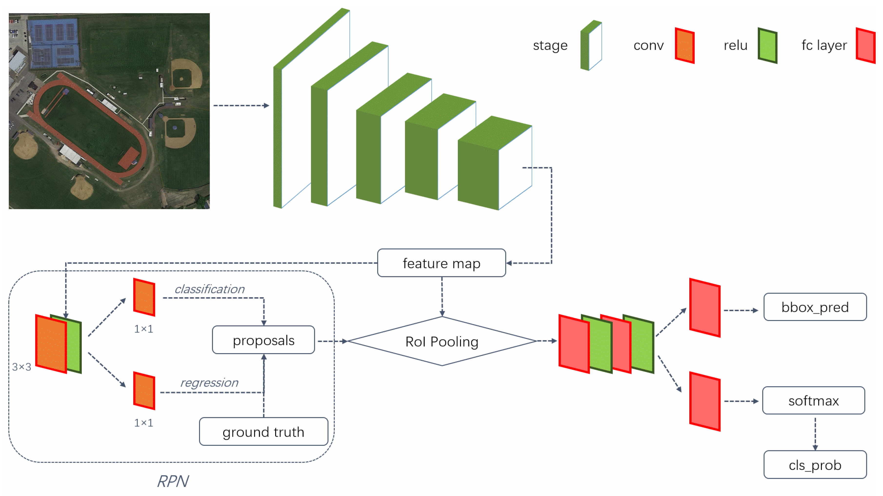
34]. Among numerous region-based methods, Region-based CNN (R-CNN) [35] is a pioneering work. It utilizes the selective search algorithm [36] to generate the region proposals, and then extracts features via CNN on these regions. The extracted features are fed into a trained SVM classifier, which classifies the category of the object. Finally, bounding box regression is used to correct the initial extracted coordinates and non-maximum uppression (NMS) is used to delete highly redundant bounding boxes to obtain accurate detection results. R-CNN [35] demands to perform feature extraction at each region proposal, so the process is time-consuming [37]. Besides, the forced image resizing process on the candidate regions before they are fed into the CNN also caused information loss. To solve the above problems, He et al. proposed Spatial Pyramid Pooling Network (SPP-Net) [
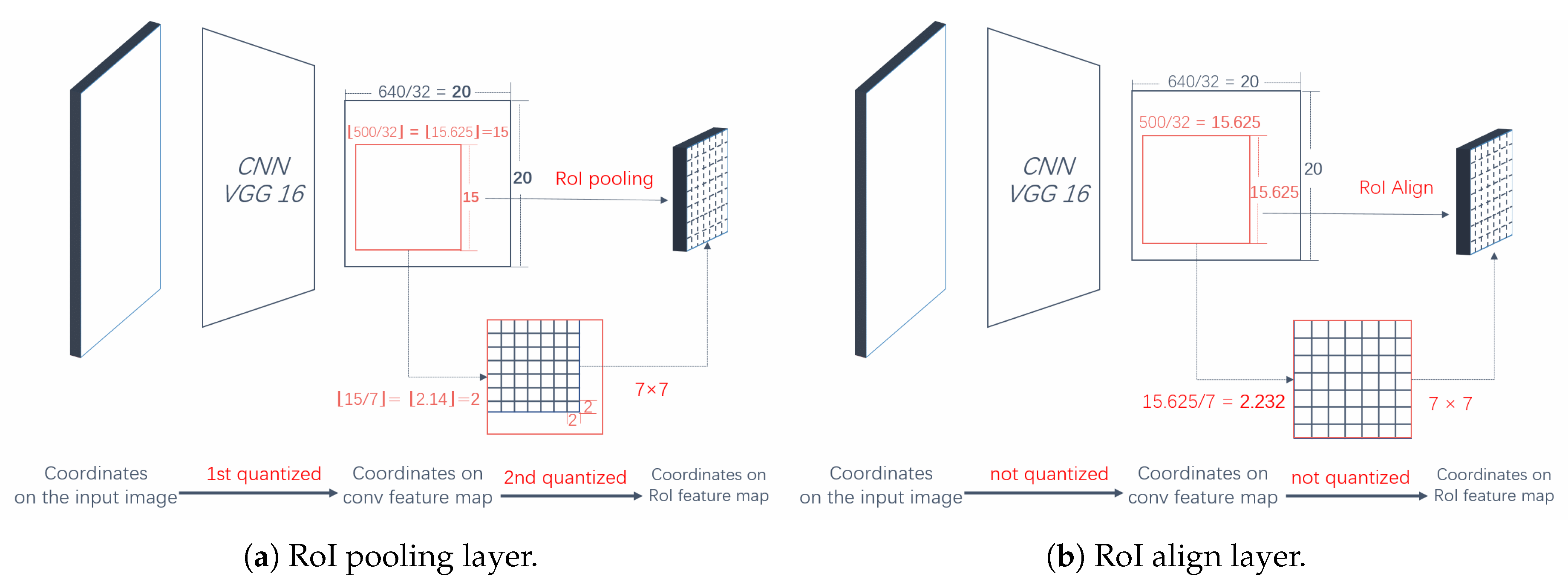
38], which adds a spatial pyramid layer, namely, Region-of-Interest (RoI) pooling layer, on the top of the last convolutional layer. The RoI pooling layer divides the features and generates fixed-length outputs, therefore it can deal with the arbitrary-size input images. SPP-Net [38] performs one-time features extraction to obtain an entire-image feature map, and the region proposals share the entire-image feature map, which greatly speeds up the detection. On the basis of R-CNN, Fast-RCNN [39] adopts the multi-task loss function to carry out classification and regression simultaneously, which improves the detection, positioning accuracy and greatly improves the detection efficiency. However, using the selective search algorithm to generate region proposals is still very time-consuming because the algorithm implements on the central processing unit (CPU). In order to take advantage of the GPUs, Faster R-CNN [
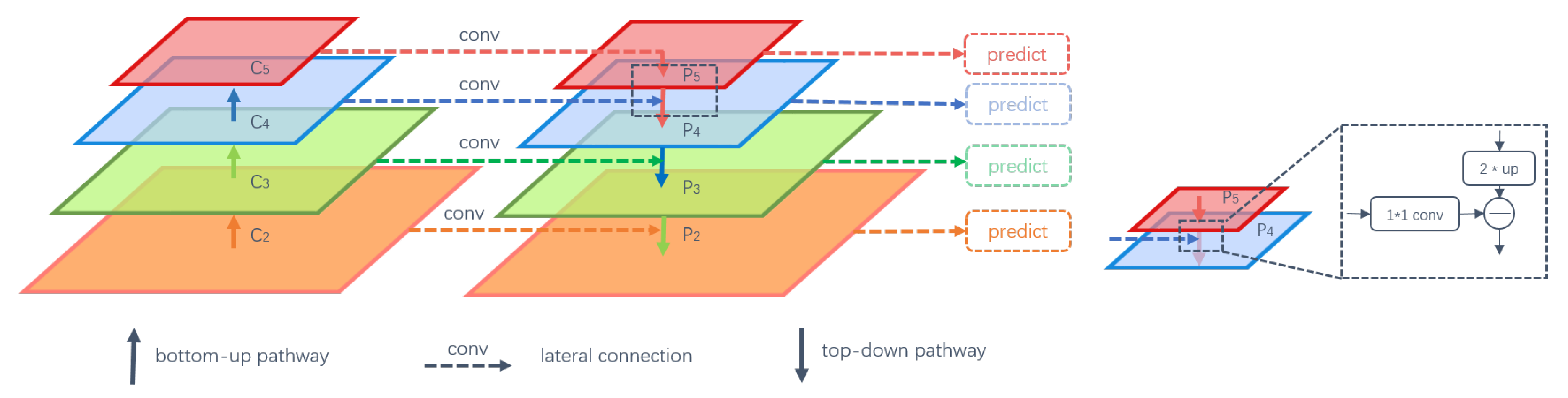
37], consisting of a region proposal network (RPN) and Fast R-CNN, was proposed. The two networks share convolution parameters, and they have been integrated into a unified network. Thus, the region-based object detection network achieves end-to-end operation. Feature pyramids play a crucial role in multi-scale object detection system, which combine resolution and semantic information over multiple scales. Feature pyramid network (FPN) [40] was proposed to simultaneously utilize low-resolution, semantically strong features and high-resolution, semantically weak features, it is superior to single-scale features for a region-based object detector and shows significant improvements in detecting small objects. In addition to the region-based object detection frameworks, there are many region-free object detection networks, including Over-Feat [41], you only look once (YOLO) [42] and single shot multi-box detector (SSD) [43], etc. These one-stage networks consider object detection as a regression problem, they do not generate region proposals and predict the class confidence and coordinates directly. They greatly improve the detection speed, although sacrificing some precision.
The CNN-based natural imagery object detection has made great progress, but high-precision and high-efficiency object detection for remote sensing images still has a long way to go. Different from natural images, remote sensing images usually show the following characteristics:
  • The perspective of view. Remote sensing images are usually obtained from a top-down view while natural images can be obtained from different perspectives, which greatly affects how objects are rendered on the images [1].
  • Overlarge image size. Remote sensing images are usually larger in size and range than natural images. Compared with natural image processing, remote sensing image processing is more time-consuming and memory-consuming.
  • Class imbalances. The imbalances mainly include category quantity and object size. Objects in natural scene images are generally uniformly distributed and not particularly numerous, but a single remote sensing image may contain one object or hundreds of objects and it may also simultaneously include large objects such as playgrounds and small objects like cars.
  • Additional influence factors. Compared with natural scene image, remote sensing image object detections are affected by illumination condition, image resolution, occlusion, shadow, background and border sharpness [33].
Therefore, constructing a robust and accurate object detection framework for remote sensing images is very challenging, but it is also of much significance. To overcome the size restrictions of the input images, the problem of small objects loss and retain the resolution of the objects, Chen et al. [1] put forward MultiBlock layer and MapBlock layer based on SSD [43]. The MultiBlock layer divides the input image into multiple blocks, the MapBlock layer maps the prediction results of each block to the original image. The network achieves a good effect on airplane detection. Considering the complex distribution of geospatial objects and the low efficiency for remote sensing imagery, Han et al. [33] proposed the P-R-Faster R-CNN, which achieves multi-class geospatial object detection by combining the robust properties of transfer mechanism and the sharable properties of Faster R-CNN. Guo et al. [3] proposed a unified multi-scale CNN for multi-scale geospatial object detection, which consists of a multi-scale object proposal network and a multi-scale object detection network. The network achieves the best precision on the Northwestern Polytechnical University very high spatial resolution-10 (NWPU VHR-10) [44] dataset. However, for small and dense objects detection on remote sensing images, they did not propose an effective solution, and did not make full use of the resolution and semantic information simultaneously, which may lead to unsatisfactory results in the case of more complex backgrounds, numerous data and overlarge image size [4,40]. Some frameworks [1,45,46,47] only have effects for certain types of objects. Besides, RoI pooling layer in these networks will cause misalignments between the inputs and their corresponding final feature maps, these misalignments affect the object detection accuracy, especially for small objects.
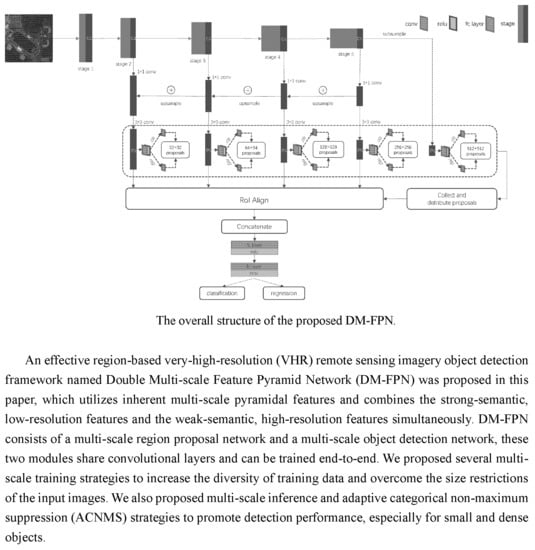
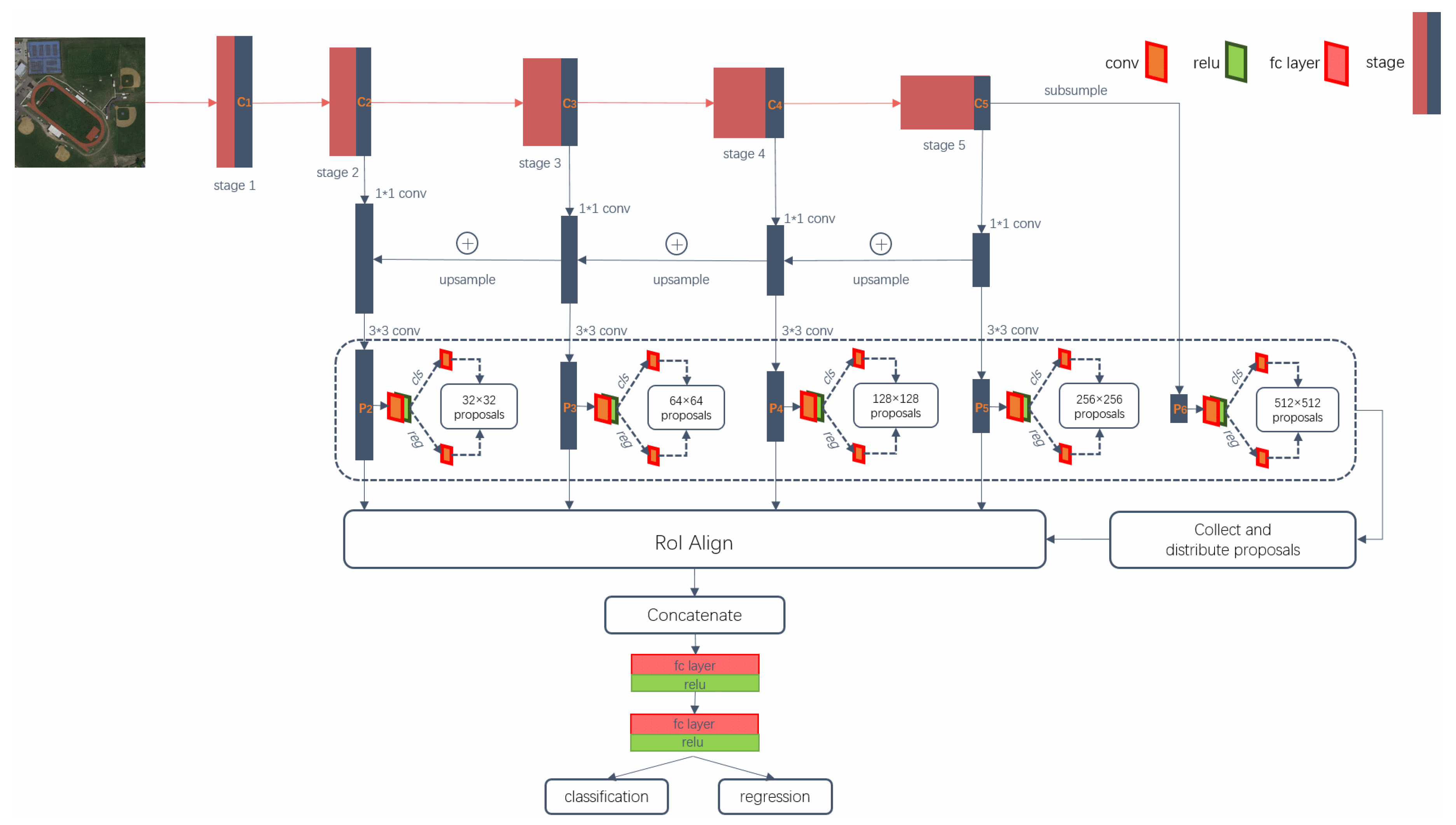
To solve the above problems, we presented an effective framework, namely, Double Multi-scale Feature Pyramid Network (DM-FPN), which makes full use of semantic and resolution features simultaneously. We also put forward some multi-scale training, inference and adaptive categorical non-maximum suppression (ACNMS) strategies. The main contributions of this paper are summarized as follows:
  • We have constructed an effective multi-scale geospatial object detection framework, which achieves good performance by simultaneously utilizing low-resolution, semantically strong features and high-resolution, semantically weak features. Accordingly, the RoI Align layer used in our framework can solve the misalignment caused by RoI pooling layer and it improves the object detection accuracy, especially for small objects.
  • We proposed several multi-scale training strategies, including the patch-based multi-scale training data and the multi-scale image sizes used during training. To overcome the size restrictions of the input images, we divided the image into blocks with a certain degree of overlap. The patch-based multi-scale training data strategy both enhance the resolution features of the small objects and integrally divide the large objects into a single patch for training. In order to increase the diversity of objects, we adopt multiple image sizes strategy for patches during training.
  • During the inference stage, we also proposed a multi-scale strategy to detect as many objects as possible. Besides, depending on the intensity of the object, we adopt the noval ACNMS strategy, which can effectively reduce redundancy among the highly overlapped objects and slightly overcome the uneven quantity distribution of training samples, enabling the framework preferably to detect both small and dense objects.
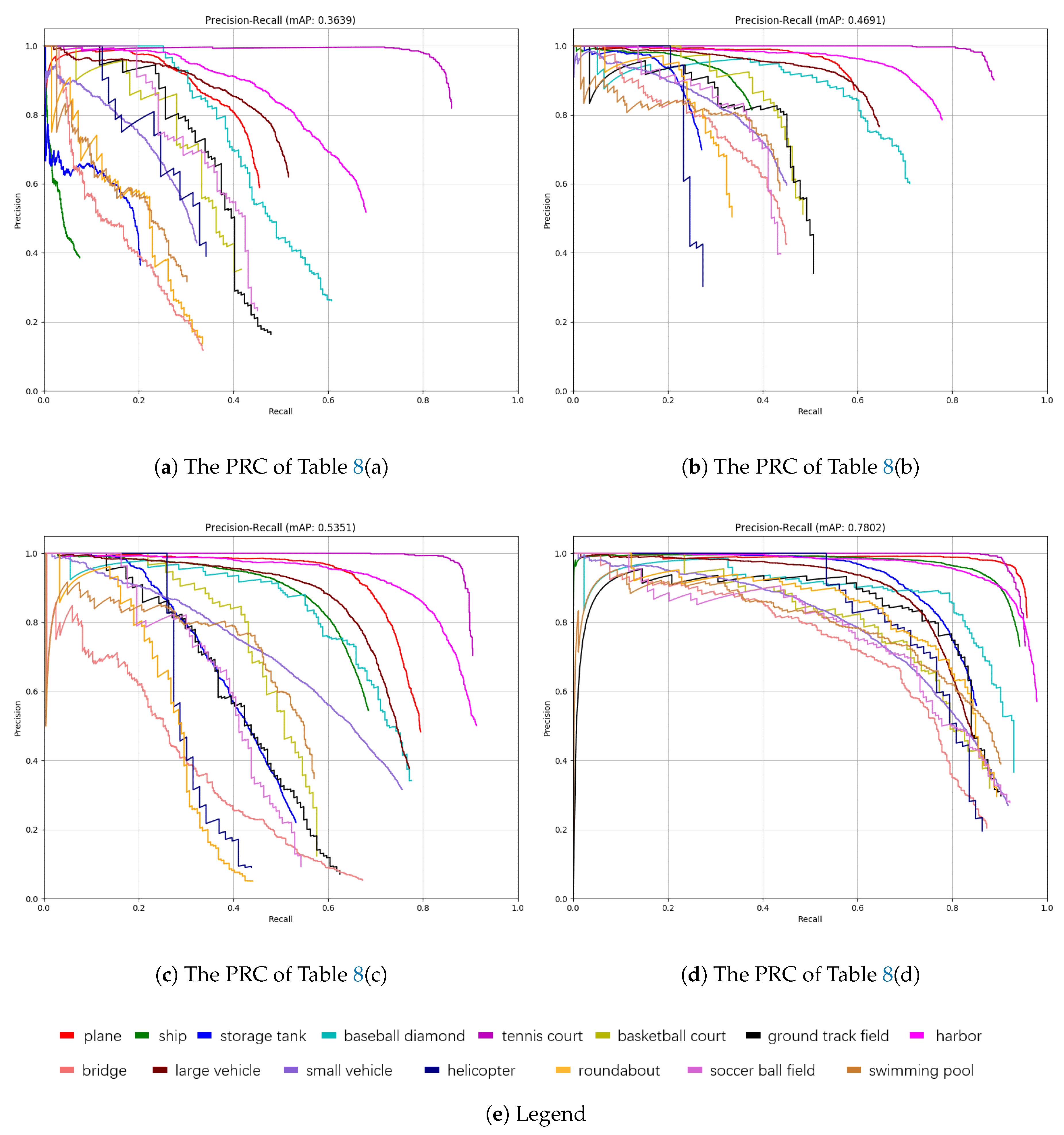
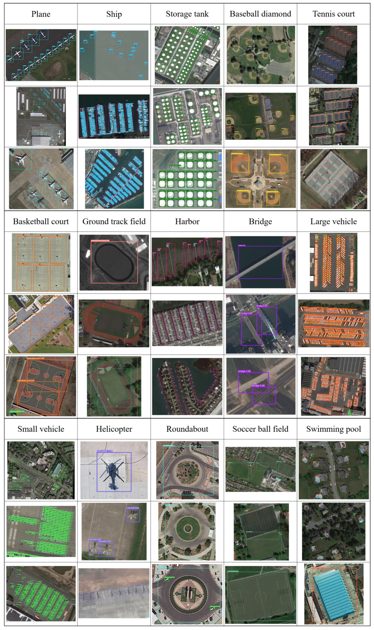
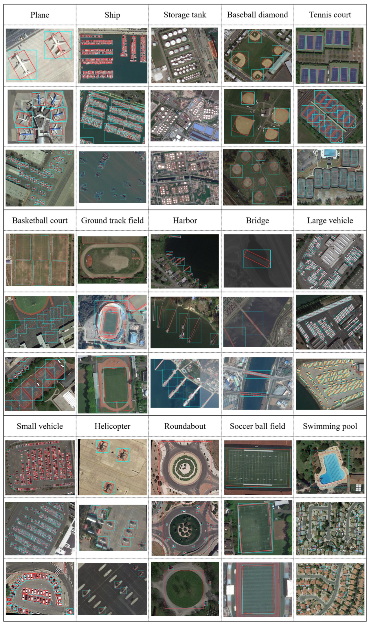
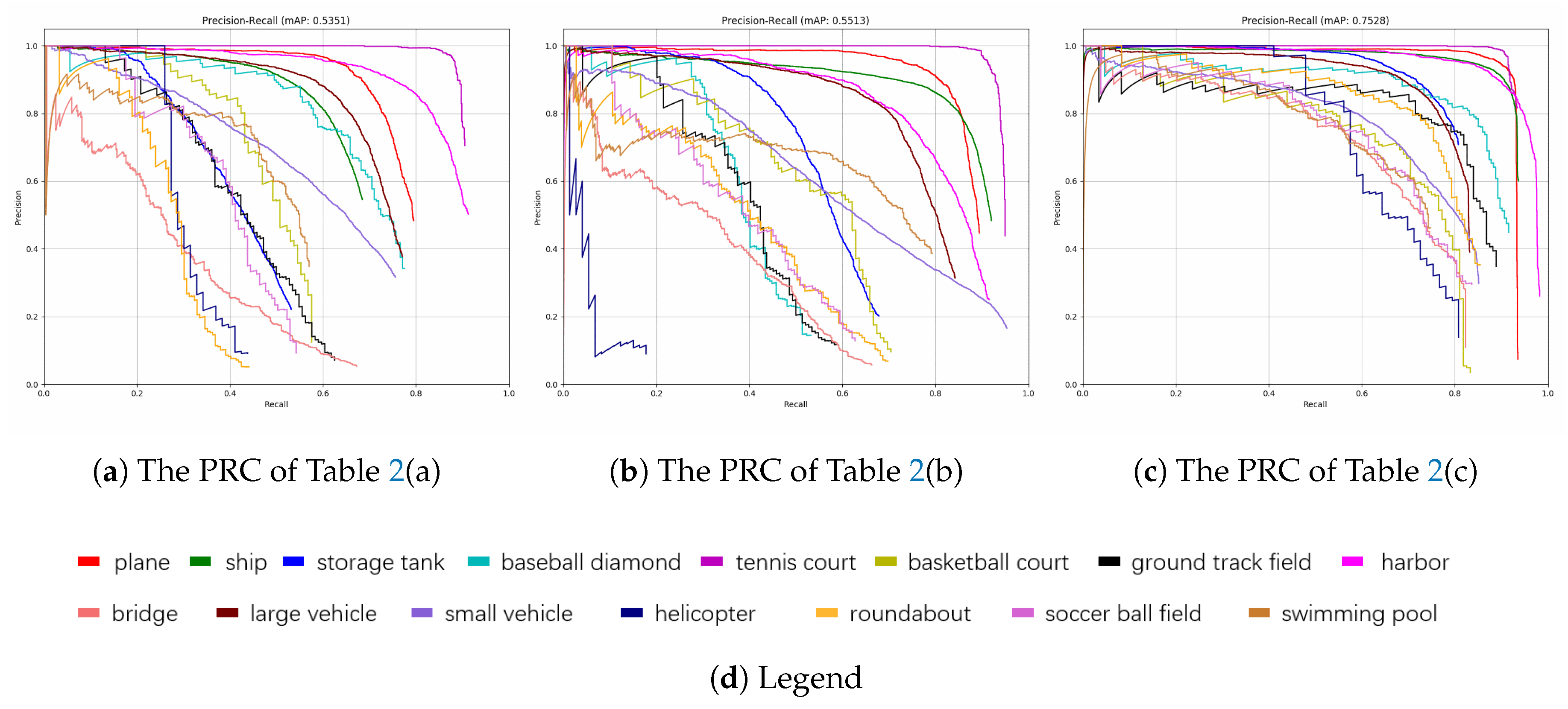
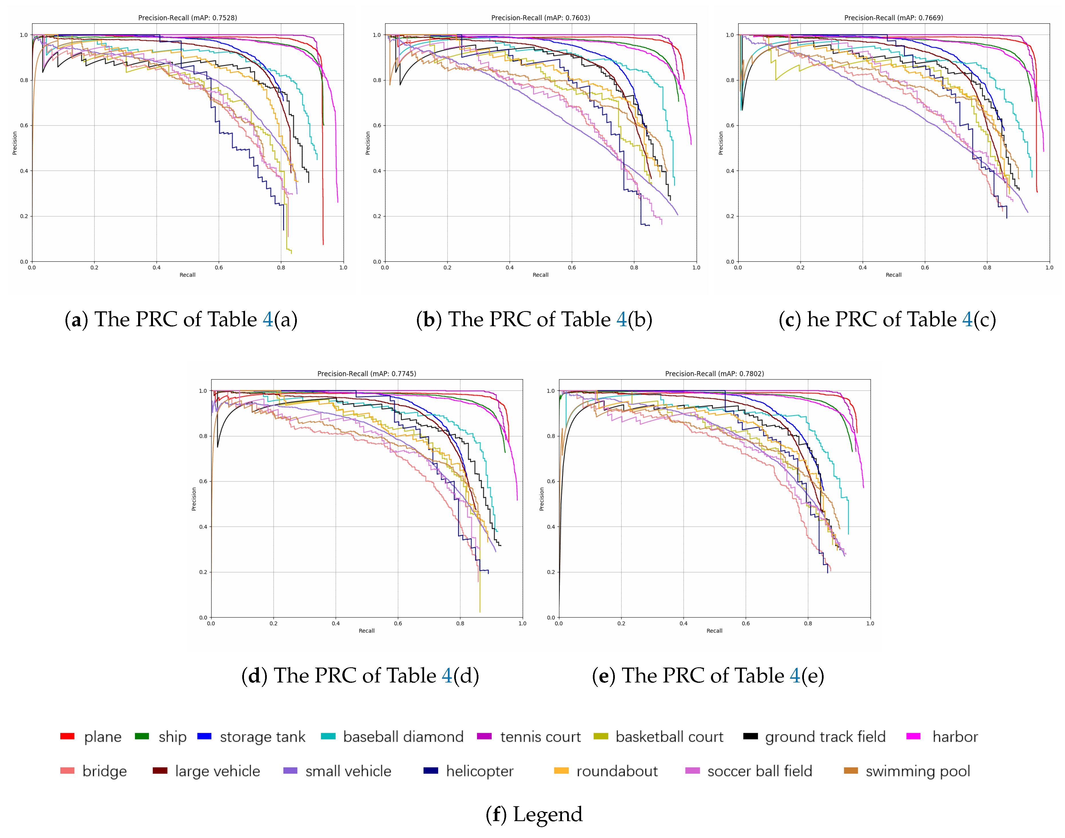
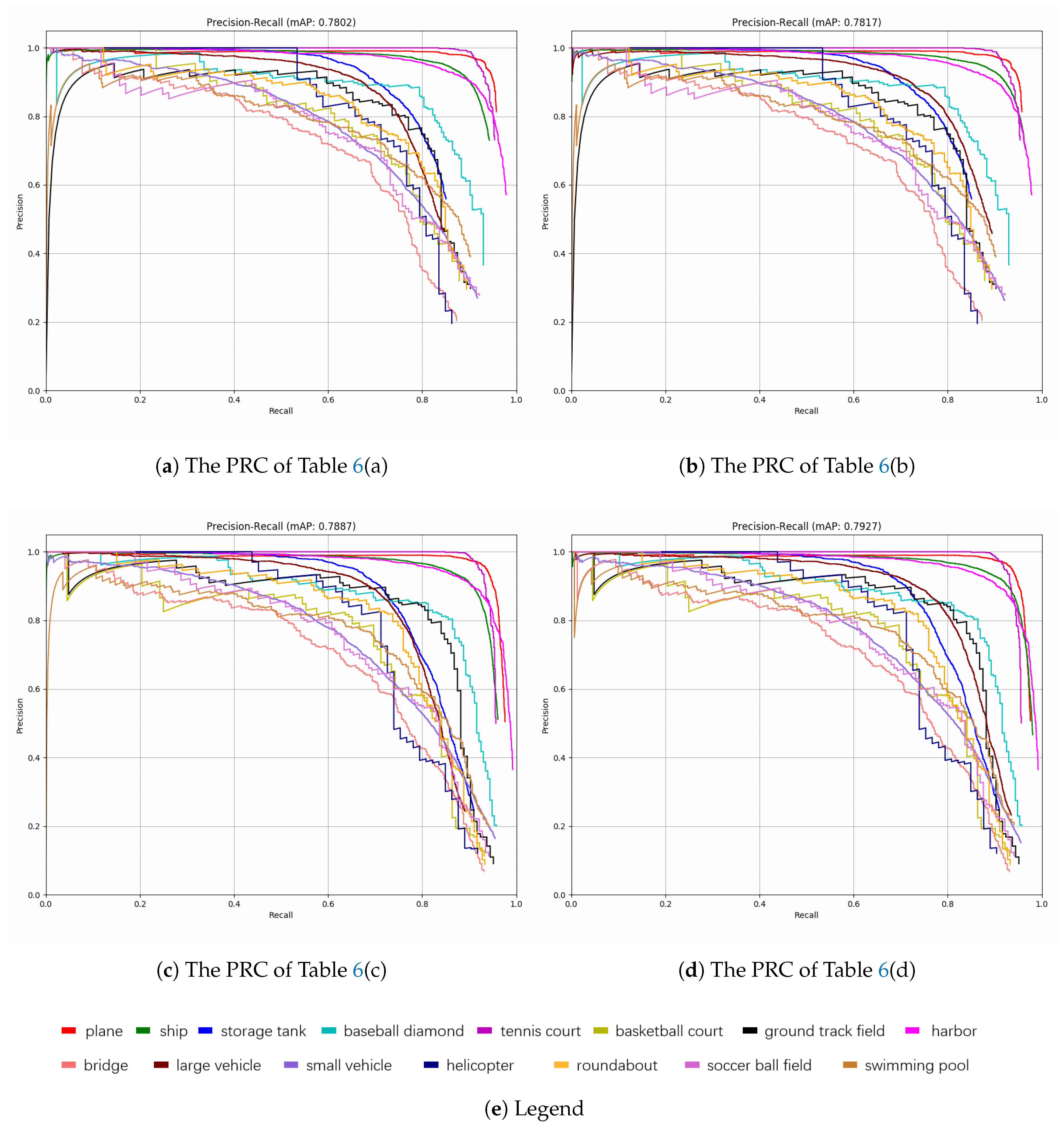
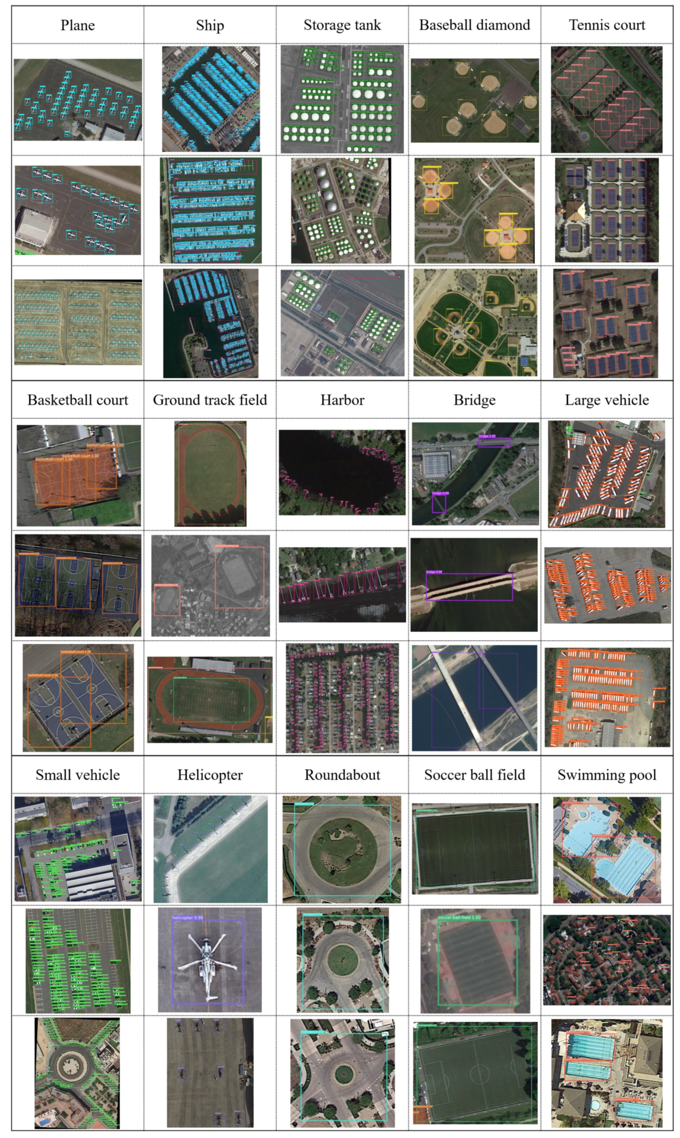
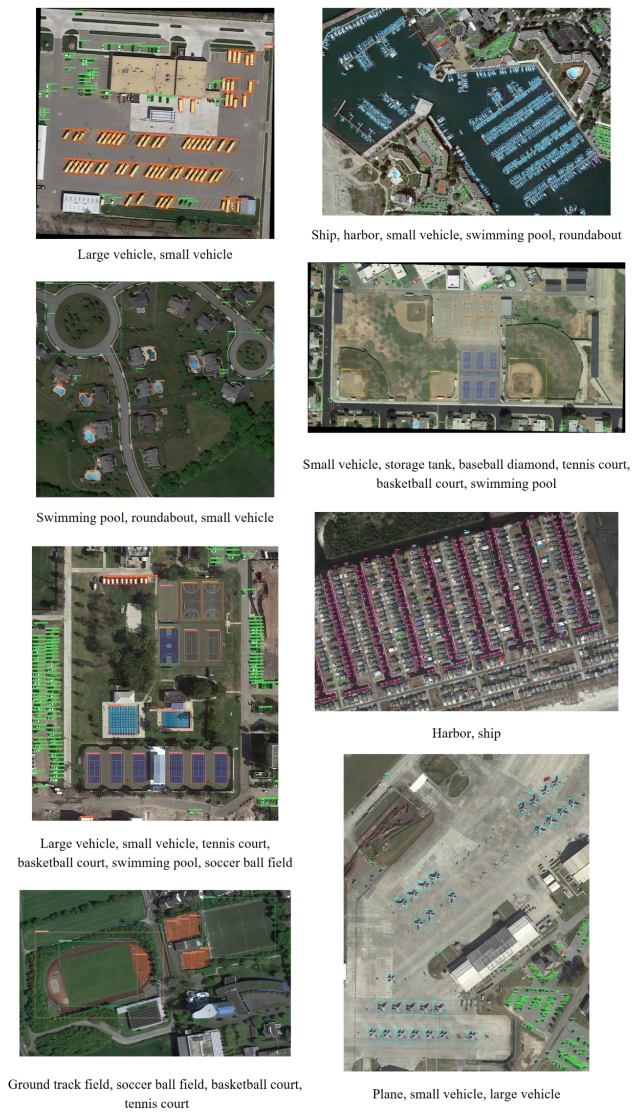
Experiment results evaluated on DOTA [48] dataset, a large-scale dataset for object detection in aerial images, indicating the effectiveness and superiority of the proposed framework. The rest of this paper is organized as follows. Section 2 introduces the related work involved in the paper. Section 3 elaborates the proposed framework in detail. Section 4 mainly includes the description of the datasets, evaluation criteria and experiment details. Section 5 implements ablation experiments and makes reliable analyses to the results. Section 6 discusses the proposed framework and analyzes its limitations. Finally, the conclusions are drawn in Section 7.

2. Related Works

In this section, we will first review some outstanding region-based object detection frameworks, they have achieved remarkable accomplishments on natural image object detection. Then we will introduce RoI Align layer, which can significantly improve the detection performance of small objects.

2.1. Region-Based Object Detection Networks

The region-based object detection networks are mainstream frameworks for high-precision object detection, including R-CNN, SPP-Net, Fast R-CNN and Faster R-CNN [35,37,38,39]. Their common process is to first generate numerous candidate areas by the region proposal algorithms [36,49,50]. Then, the networks employ CNN to extract abundant features from these candidate regions and infer the category and coordinates of objects on each region. Finally, a bounding box algorithm is utilized to get precise coordinates. Faster R-CNN integrates these steps to form a unified network and realizes end-to-end object detection. It consists of two modules, formally, RPN and Fast R-CNN, and the two tasks share convolutional features. Figure 1 shows the overall architecture of Faster R-CNN.
RPN is a kind of fully convolutional network [51], it deals with the arbitrary-size input image and outputs a set of region proposals with an objectness score. These candidate regions will be fed into the following Fast R-CNN for precise detection. The core scheme of RPN is “anchors”, which simultaneously predicts multiple region proposals of diversiform scales and aspect ratios with a total number of k at each sliding window in the last shared convolutional layer. The features obtained from each sliding window will be imported into two sibling 1 × 1 convolutional layers, specifically, the box-classification layer (cls) and the box-regression layer (reg). The cls layer is used to identify a binary class label of being an object or not while the reg layer is used to correct the coordinates of the object. Therefore, the cls layer has 2k outputs while the reg layer has 4k outputs.
After RPN processing, we got a mass of candidate regions with class-agnostic and coordinate attributes. These regions will be fed into the subsequent Fast R-CNN for further category judgment and coordinate regression. Fast R-CNN adopts RoI pooling layer to extract fixed-length feature vectors from arbitrary-size candidate regions and these feature vectors are fed into categorical classification and regression layers to obtain the final detection results. The RPN and Fast R-CNN employ the approximate joint training scheme to share convolution. As such, an efficient and end-to-end object detection framework is constructed.

2.2. Feature Pyramid Network

Most region-based object detection frameworks only use the single-scale features for faster detection, such feature representations are very unfriendly to small objects. In Faster R-CNN, the backbone adopts Visual Geometry Group 16 weight layers (VGG16 [52]) and the last feature map reduces to 1/32 compared to the original image after 5 convolutional layers (with a pooling step of 2), some small objects like cars and ships will lose a large proportion of features after such operations. In the deep convolutional networks, the low-level layers have poor semantic but strong resolution while the high-level layers have rich semantic but scarce resolution [40]. Although some frameworks [43,53] adopt multi-scale feature maps that already computed from different layers, they abnegate low-level features and therefore lose the opportunity to take advantage of higher-resolution features. Combining strong resolution and semantic information will enhance the detection performance, especially for small objects. In a pioneering way, FPN leverages the in-network features obtained from the last layer of each stage in the convolutional networks (ConvNets). It combines coarse-resolution, semantically strong features with high-resolution, semantically weak features to construct a multi-scale pyramidal hierarchy network without additional memory consumption. We note that if the output feature maps have the same size, they are in the same stage. As shown in the Figure 2, the core mechanism of the FPN mainly includes bottom-up pathway, top-down pathway and lateral connections.
  • Bottom-up pathway. Actually, this operation is the forward propagation process of the network. During the operation, the last convolutional layer in each stage is extracted to establish a feature pyramid. Compared with other methods [54,55,56], this mechanism requires no additional memory footprint.
  • Top-down pathway and lateral connections. The top-down pathway upsamples the feature map obtained from the bottom-up pathway to the same size as the semantically coarser, but spatially stronger feature maps. The lateral connections merge the same-size feature maps obtained from the bottom-up pathway and the top-down pathway respectively, which first undergoes a 1 × 1 convolutional layer to reduce channel dimensions. The mergence process is implemented by element-wise addition. Subsequently, a 3 × 3 convolution is executed on each merged feature map to eliminate the aliasing effect of upsampling.

2.3. ROI Align

ROI Align is a kind of regional feature aggregation method proposed in Mask R-CNN [57], which solves the problem of misalignment caused by RoI pooling during the two integer quantification operations. RoI pooling layer divides the region proposal on the last convolutional layer into a fixed-length (e.g., 7 × 7 ) feature map for subsequent classification and bounding box regression tasks. Since the coordinates of candidate regions are obtained by regression, generally speaking, they are floating-numbers. After rounding down, the data after the decimal point is abandoned. As shown in Figure 3a, there are two rounding operations during the pooling: the coordinates of candidate region are first quantified to integer, then the quantified RoI is divided into k × k bins on average, and each bin is quantified again thus introducing misalignments between the RoI and the final feature map. Such misalignments are harmful to objects detection task, especially for small objects.
RoI Align was proposed to solve the above deficiency of RoI Pooling, it abnegates all quantifications and utilizes bilinear interpolation to obtain the precise values. Formally, RoI Align retains the original floating-numbers instead of quantified integers. The alignment process is shown in Figure 3b. During the first quantification, the boundary coordinates of each candidate region are not round down to maintain floating-numbers. During the second quantification, each RoI is divided into k × k bins and this process is still not round down. Subsequently, four fixed sampled points are calculated by bilinear interpolation in each RoI bin, and the maximum or average pooling is performed to get align results. RoI Align solves the misalignments between the inputs and the extracted feature maps, which is significant for object detection on remote sensing images that contain numerous small objects.

3. Framework

In this section, we will elaborate the details of our proposed framework. In order to efficiently detect the objects on remote sensing images, we also propose some multi-scale training and inference strategies. Meanwhile, different ACNMS thresholds are selected according to the size and intensity of the category, which can improve the detector performance to some extent.

3.1. The Core Mechanism of the Proposed Network

3.1.1. The Overall Structure

The overall structure of the proposed framework named Double Multi-scale Feature Pyramid Network (DM-FPN) is shown in Figure 4.
The infrastructure of DM-FPN is based on Faster R-CNN [37] with FPN [40]. Formally, both the original region proposal network and the detection network were modified by FPN. DM-FPN combines coarse-resolution, semantically strong features with high-resolution, semantically weak features, and such operations have great advantages in detecting small objects. We adopt ResNet50 [58] as backbone of our framework. The convolution can be divided into 5 stages and the output of each stage’s last residual block was selected as {C 2 , C 3 , C 4 , C 5 }, noting that they have strides of {4, 8, 16, 32} pixels corresponding to the original image. We do not utilize the first stage because it is memory-consuming. This process is called the bottom-up pathway, which has been described in Section 2.2. The corresponding {P 2 , P 3 , P 4 , P 5 } were obtained by top-down path, lateral connections and mergence. Actually, to eliminate the aliasing effect of upsampling, a 3 × 3 convolution is executed on each merged feature map to obtain the final feature maps {P 2 , P 3 , P 4 , P 5 }, which are shared by the region proposal network and the class-specific detection network.

3.1.2. Multi-Scale Region Proposal Network

The original RPN extracts region proposals on the last single-scale convolutional layer. In order to take advantage of the pyramid character of FPN, we need to extract candidate regions on multiple convolutional layers, namely, {P 2 , P 3 , P 4 , P 5 , P 6 }, noting that P 6 is simply a stride 2 subsampling of P 5 , which is only used in multi-scale region proposal network. The anchors own ranges of {32 2 , 64 2 , 128 2 , 256 2 , 512 2 } pixels on {P 2 , P 3 , P 4 , P 5 , P 6 } respectively. On each feature map, there are three aspect ratios, namely, {1:2, 1:1, 2:1}. As a result, there are a total of 15 anchors on these pyramidal feature maps. The selection of positive and negative samples is determined by the Intersection-over-Union (IoU) between the region proposal and ground-truth box. We note that IoU is defined as the ratio between the intersection and the union of two boxes. If an anchor has the highest IoU with a given ground-truth box or it has an IoU greater than 0.7 with any ground-truth box, then it will be assigned to the positive. Conversely, if an anchor has an IoU less than 0.3 for all ground-truth boxes, it’s a negative sample. We abandon samples that are neither positive nor negative. In a mini-batch of 256, the ratio of positive to negative samples is 1:1. These rules apply to {P 2 , P 3 , P 4 , P 5 , P 6 } indistinguishably. Specially, the common ground-truth boxes are equally participated in the calculation with the pyramid anchors located on five-level feature maps. With these definitions, the loss function for an image is defined as:
L { p i } , { t i } = 1 N c l s i p i , p i * + λ · 1 N r e g i p i * L r e g t i , t i *
where i represents the index of an anchor in a mini-batch while p i is the predicted probability of anchor i being an object. If the anchor is positive, the ground-truth label p i * equals to 1, otherwise equals to 0. t i is a vector that consists of four parameterized coordinates of the predicted bounding box, and t i * is that of the ground-truth box associated with a positive anchor. The classification loss L c l s is represented by the log loss, which identifies a binary class label of being an object or not. And the regression loss L r e g is constructed by the Smooth L1 loss. The above two loss functions are weighted by a balancing parameter λ . Usually, the cls term is normalized by the mini-batch size while the reg term is normalized by the number of anchors. In this paper, we specify that N c l s and N r e g are equal to 256 and 2000, respectively. We set λ is equals to 9 and thus both cls and reg terms are roughly equally weighted.
We note that we reserve the top 2000 region proposals based on their cls scores on {P 2 , P 3 , P 4 , P 5 , P 6 } respectively, then we concatenate these candidate boxes and adopt Non-Maximum Suppression (NMS) with a fixed IoU threshold of 0.7 to retain the final 2000 RoIs, which will be fed into the subsequen class-specific detection network for exact object detection.

3.1.3. Multi-Scale Class-Specific Detection Network

Fast R-CNN [39] is a single-scale region-based object detection framework, which utilizes RoIs generated by RPN for object detection. Different from the previous networks that pooling RoI to single-scale feature map, we need to align RoIs from different scales to the multiple pyramidal feature maps. We assign an RoI of width w and height h (based on the input image) to the level P k by:
k = k 0 + log 2 ( w h / 224 )
where 224 is the normative ImageNet pre-training size as FPN [40] does, and k 0 is the level that an RoI with a size of w × h = 224 2 should be mapped into. Notably, we assigned k 0 equals to 4 as [40] does. These RoIs can be assigned to different levels according to their size. For example, if an anchor has a width of 188 and a height of 111, it should be mapped into the P 3 level. Subsequently, we adopt RoI align to extract 7 × 7 feature maps, which will be fed into two 1024-d fully-connected layers before the final classification and bounding box regression layers. Based on the above settings, both region proposal network and class-specific detection network can utilize multi-scale pyramidal features for object detection.

3.2. Multi-Scale Training Strategies

Multi-scale training strategies mainly include the patch-based multi-scale training data and the multi-scale image sizes used during training. Their descriptions are as follows:
  • Patch-based multi-scale training data. The size restrictions of the input images cause a lot of semantic information will lost in the deep convolutional layers, especially for small objects. Therefore, we slice remote sensing images into patches with a certain degree of overlap, and then send these image blocks into the network for training. At the same time, considering the uneven distribution of objects on the remote sensing image, which may include large objects such as playgrounds, and may also include small objects like cars, we enlarge and shrink remote sensing images by a factor of 2 and 0.5 respectively. The enlarged remote sensing images enhance the resolution features of the small objects while the shrunken remote sensing images integrally divide the large objects into a single patch for training.
  • Multi-scale image sizes used during training. In order to enhance the diversity of objects, we adopt multiple scales for patches during training. Each scale is the pixel size of a patch’s shortest side and the network uniformly select a scale for each training sample at random.

3.3. Multi-Scale Inference Strategies

We scale images to detect as many objects as possible during inference, and the scaled images include enlarged and shrunken images, horizontally and vertically flipped images. Specifically, we first perform multi-scale process on each test image, then we slice it into patches with a certain degree of overlap according to its size and carry out detection on these image blocks. Finally, we apply ACNMS to these concatenate bounding boxes from each patch to get the final results.

3.4. Adaptive Categorical Non-Maximum Suppression (ACNMS)

NMS is a post-processing module in the object detection framework, which is mainly used to delete highly redundant bounding boxes. A single remote sensing image may contain one big object or hundreds small objects, thus there exists a class imbalance between different categories. In the previous multi-class object detection works [3,4,33], the NMS thresholds for different categories are the same, but we find that different NMS thresholds for different categories based on the category intensity (CI) can improve the accuracy of object detection to a certain extent. We define CI as:
C I = N I o C / N i m g
where N I o C means the total number of instances for each category, N i m g means the total number of images. If the CI of a category is greater than the given threshold, we set this category a larger NMS threshold than the generic NMS threshold. In general, NMS thresholds for denser objects are larger because they overlap each other more commonly.

4. Dataset and Experimental Settings

4.1. Dataset Description

We evaluated our proposed framework on DOTA [48] dataset, which contains 2806 aerial images with pre-divided 1411 training images, 458 validation images and 937 testing images. We note that the testing images have no labels, however, you can submit the test results in a fixed format to DOTA Evaluation Server (http://captain.whu.edu.cn/DOTAweb/evaluation.html). Those DOTA images are obtained from different sensors and platforms with crowdsourcing and the size ranges from 800 × 800 to 4000 × 4000 pixels. DOTA consists of 15 common categories, namely, plane, ship, storage tank, baseball diamond, tennis court, basketball court, ground track field, harbor, bridge, large vehicle, small vehicle, helicopter, roundabout, soccer ball field and swimming pool. The fully annotated DOTA dataset contains 188,282 instances, each of which is labeled by an oriented quadrilateral instead of an axis-aligned one, which is typically used for object annotation in natural scene images. Another common geospatial object detection dataset is NWPU VHR-10 [44], which contains 800 images in 10 categories with a total of 3651 instances. The average size of NWPU VHR-10 is 1000 × 1000 pixels. Compared with NWPU, DOTA is a larger annotated dataset for multi-class geospatial object detection, which has more complex backgrounds, larger image size and denser object distribution thus more reflective of the real-world applications [48]. Therefore, the evaluation on DOTA can better verify the effectiveness and robustness of our proposed network.
The benchmark of DOTA contains two detection tasks. Task 1 uses the initial oriented bounding boxes as ground truth. Task 2 uses the converted horizontal bounding boxes as ground truth. In this work, we only focus on the horizontal bounding box detection task with ( x m i n , y m i n , x m a x , y m a x ) format, so we need to convert the labeled oriented bounding box into the minimum bounding rectangle for each image. Figure 5 shows some examples about the original annotations and their minimum bounding rectangles.

4.2. Evaluation Criteria

We adopted Precision-Recall Curve (PRC) and Average Precision (AP) as evaluation criteria in our experiments, which are widely used in the object detection works.

4.2.1. Precision-Recall Curve

The precision metric is the ratio of the correct identification quantity to the total identification quantity while the recall metric is the proportion of the correct identification quantity to the total labeled quantity, which can be illustrated by the following two formulas:
p r e c i s i o n = T P / ( T P + F P )
r e c a l l = T P / ( T P + F N )
we note that if the IoU value between the predicted bounding box and the ground truth is larger than 0.5, it will be considered as true positive ( T P ) , otherwise, it will be considered as false positive ( F P ) . In addition, false negative ( F N ) refers to the prediction boxes that overlap with ground truth but do not have the maximum overlap value. The precision-recall curve (PRC) describes the relationship between the precision metric and the recall metric, an object detector of a certain category is considered good if its prediction stays high as recall increases.

4.2.2. Average Precision

Average Precision (AP) is the averaged precision across all recall values between 0 and 1, namely, the area under the PRC. A higher AP indicates a better detector. Mean average precision(mAP) represents the average AP over all categories.

4.3. Baseline Methods

We compared the proposed framework with the classic region-based methods including Faster RCNN [37] and FPN [40] on DOTA validation dataset. For the testing dataset, we submitted the inference results to DOTA website because of lacking annotated labels, and we selected several current top-ranked results for comparison.

4.4. Implementation Details

We implemented our network on the open source Caffe2 (https://caffe2.ai/) framework and executed on a 64-bit Ubuntu 16.04 computer with 8GB memory GeForce GTX1070Ti GPU. We note the comparison models were implemented in their original environments without any additions.

4.4.1. Training

We first enlarged and shrunk the original images by a factor of 2 and 0.5 respectively, then we sliced the original and scaled images into patches of 1000 × 1000 pixels with an overlap of 500 pixels. All the original image patches, partial randomly selected enlarged and shrunken image patches were taken as our training samples with a total number of 31,396. These training samples will be fed into the network after data augmentation, which includes rotation and flip. We adopted three scales during training, they are 800 × 800 , 900 × 900 and 1000 × 1000 pixels respectively. Each scale is the pixel size of a patch’s shortest side and the network uniformly select a scale for each training sample at random. We adopted ResNet50 as our backbone, which was pre-trained on ImageNet dataset. We trained a total of 300k iterations with a learning rate of 0.0025 for the first 150k iterations, 0.00025 for the next 50k iterations, and 0.000025 for the remaining 100k iterations, which took us about 40 hours in total. The network was trained by stochastic gradient descent algorithm with a mini-batch of 2 images. Weight decay and momentum are 0.0001 and 0.9 respectively.

4.4.2. Inference

We implemented inference based on the image patches in order to detect as many objects as possible. To accelerate the inference, we sliced validation images into patches of 1000 × 1000 pixels with an overlap of 200 pixels. We performed detection on each diced image and then concatenated the predicted results from each patch. We set CI threshold to 10, and the ACNMS threshold is 0.38. Specifically, if the intensity of a category is greater than CI threshold, then its NMS threshold is 0.38, otherwise we set its NMS threshold to 0.3. Meanwhile, to verify the effectiveness of the multi-scale inference strategies, we also performed the same detections on the shrunken images, the horizontal rotation and vertical rotation images simultaneously. We did not perform detections on the enlarged images because of their vastly time-consuming.

5. Results and Analysis

5.1. Ablation Experiments

Ablation experiments were carried out to verify the effectiveness of the proposed multi-scale training, inference and ACNMS strategies. In the following subsection, we will gradually verify the relevant strategies. The multi-scale training and inference strategies can be expressed as Equation (6):
( p ) _ b a s e d ( x ) + ( s ) _ s c a l e
where p represents the patch sizes used for training, x represents the patch sources used for training and s represents the patch scales used for inference. For example, 800_based(4)+1_scale means that we resized the pre-divided patches into 800 × 800 pixels for training. These multi-scale training data include four data sources, specifically, the original images, the patches obtained from original images, enlarged and shrunken images. During inference, we performed detection on the patches only obtained from original images. The size of these patches is 1000 × 1000 pixels with an overlap of 200 pixels. Finally, we concatenated the bounding boxes from each patch and adopted ACNMS to get the final results. The detailed explanations are shown in Table 1.

5.1.1. Patch-Based Training and Inference Strategies

In this section, we conducted two sets of ablation experiments to illustrate the superiority of patch-based training and inference strategies. We adopted (a), (b), (c), etc. to represent each method in Table 2. In each column, the bold number indicates the best detection result, and the other tables are the same. Table 2(a) carried out training using the original images without patches. For fair comparison, we resized the original images to 1000 × 1000 pixels and the inference was also performed on the original images. The training strategies of Table 2(b) were the same as Table 2(a), however, it performed inference on the patches obtained from the original images. Both training and inference of Table 2(c) were performed on the patches obtained from the original images.
Comparing Table 2(a) and Table 2(b), we can observe that patch-based inference strategy has improved detection accuracy on most categories except baseball-diamond, ground-track-field, harbor, helicopter and soccer-ball-field. Through further experiments we found that the sizes of baseball-diamond, ground-track-field, harbor, and soccer-ball-field are so large that they often beyond the scope of a single patch, therefore, training with original images but prediction with patches are not conducive to these objects. However, the poor detection effect of helicopter is mainly caused by: (1) Quite a few samples, the sample number (630) of helicopter is far fewer than other categories; (2) Some helicopter samples are similar to airplane, and these two categories generally appear simultaneously. Nevertheless, the patch-based inference strategy is still slightly ascending.
With the patch-based training strategy, Table 2(c) shows the superiority compared to Table 2(b), it not only has an overwhelming advantage in mAP (0.5513 to 0.7528), but also increases the AP value of each category, which illustrates that the patch-based training strategy is targeted and more adequately understand the characteristics of the objects. Besides, the patch-based training strategy implicitly increases the sample number of each category, especially for the sample-scarce categories.
Computational efficiency is also an important indicator in evaluating a framework’s performance, so we calculated the average running time for each strategy. The results are shown in Table 3.
We note that the patch-based inference strategies (Table 3(b),(c)) consume more average running time than the original-image-based inference strategy (Table 3(a)), which is easy to understand because the patch-based inference strategy handles more images (patches). In addition, Table 3(c) takes less time than Table 3(b), which further demonstrates that the patch-based training strategy can more adequately extract the characteristics of the objects. The quantified PRCs over two ablation experiments are plotted in Figure 6.

5.1.2. Multi-Scale Training Data and Multi-Scale Sizes Used during Training Strategies

Multi-scale training data consist of the original images, patches that based on the original images, the enlarged images and the shrunken images. Multi-scale sizes used during training refers to that an image or patch will be resized to a random scale from specified range before being fed into the framework and each scale is the pixel size of an image or patch’s shortest side. We performed two relevant ablation experiments to verify the significance of multi-scale training data and multi-scale sizes used during training. The results are shown in Table 4.
The training data used in the Table 4(a) are only from the original images while the training data used in the remaining groups include the original images, the patches from the original images, the enlarged images and the shrunken images. Table 4(b)–(d) resize the training data to 800 × 800 , 900 × 900 , 1000 × 1000 pixels respectively. Table 4(e) utilizes multiple sizes including (800, 900, 1000) pixels, and the training data will be resized to a randomly selected size before being fed into the network. Apart from this, all experiment settings and inference strategies are identical.
Combining Table 4(a) and Table 4(d), we can find that multi-scale training data can really improve the accuracy (0.7528 to 0.7745), especially for large-size categories such as basketball-court (0.6671 to 0.7275), ground-track-field (0.7225 to 0.7966) and sample-scarce category such as helicopter (0.654 to 0.7222). The accuracy of Table 4(e) is higher than Table 4(b)–(d), which indicates that multi-scale training sizes are helpful in improving the accuracy. Comparisons between Table 4(b)–(d) illustrate that the larger the training image size, the higher the detection average accuracy.
Table 5 shows computational efficiency of multi-scale strategies. Similarly, the comparison between Table 4(a) and Table 4(d) illustrates that multi-scale training data improve the framework performance to a certain extent, so it performs better in terms of computational efficiency. The comparisons between the last four groups reveal that multi-scale sizes used during training not only improve the detection performance but also improve the computational efficiency.
The quantified PRCs over multi-scale training data and multi-scale sizes used during training are plotted in Figure 7.

5.1.3. Multi-Scale Inference and ACNMS Strategies

We performed multi-scale inference on the original images, the shrunken images, the horizontal rotation and vertical rotation images simultaneously. For small and dense objects mainly including ship, large vehicle and small vehicle, we appropriately increase the NMS threshold according to their CI. The common NMS threshold is 0.3 while the ACNMS threshold is 0.38. The results are shown in Table 6.
We note that the top right corner “+” in Table 6(b),(d) indicate that we utilized ACNMS strategy. The two comparisons between Table 6(a) and Table 6(c), Table 6(b) and Table 6(d) illustrate the effectiveness of multi-scale inference strategy, which has improved detection performance both in large and small objects such as storage tank, ground track field and roundabout. The two comparisons between Table 6(a) and Table 6(b), Table 6(c) and Table 6(d) illustrate the effectiveness of ACNMS strategy. We slightly improved the NMS threshold of ship, large vehicle and small vehicle because their CIs are far greater than other’s. Specifically, the AP values of ship increase by 0.003 and 0.002 respectively in two comparison experiments, the AP values of large vehicle increase by 0.002 and 0.0055 respectively while the AP values of small vehicle remain unchanged. The relevant comparisons illustrate that increasing NMS threshold according to the category intensity does improve the detection accuracy.
Table 7 shows computational efficiency of multi-scale inference and ACNMS strategies. We note that the average running time of multi-scale inference is about three times longer than that of single-scale inference because the number of image (patch) processed by multi-scale inference is about three times more than that of single-scale inference. In addition, using ACNMS strategy does not increase additional average running time.
The quantified PRCs over multi-scale test and adaptive category NMS strategies are plotted in Figure 8.

5.2. Comparison with Other Methods

5.2.1. Comparison with Other Methods on DOTA Validation Dataset

We compared our framework with other region-based object detection networks mainly including Faster R-CNN [37] and FPN [40] on DOTA validation dataset. The selected networks had the same experimental settings as ours, however, they did not adopt our multi-scale training, inference and ACNMS strategies. Table 8 shows the comparison of different networks on DOTA validation dataset.
We note that Faster R-CNN, FPN and Table 8(c) performed training and inference on the original images instead of patches. The proposed framework has an overwhelming advantage in mAP and AP values of each category. The mAP of Table 8(c) is 0.1712 higher than that of Faster R-CNN and 0.066 higher than that of FPN, which illustrate the superiority of the proposed network. The mAP of Table 8(d) is 0.4163 higher than that of Faster R-CNN, 0.3111 higher than that of FPN and 0.2451 higher than that of Table 8(c), which illustrate the great superiority of the proposed network and the multi-scale training, inference and ACNMS strategies. The framework has great advantage in detecting small and dense objects such as ship, large vehicle, small vehicle and storage tank. The detection accuracy of sample-scarce objects such as helicopter and roundabout have also been greatly improved, which further confirms that the proposed framework has outstanding performance in detecting both small dense objects and large-scale objects.
The computational efficiency of different frameworks on DOTA validation dataset are shown in Table 9. There is no doubt that the first three groups consume less time than the last group because they performed training and inference on the original images instead of numerous patches. Besides, the proposed DM-FPN (Table 9(c)) can achieve higher object detection accuracy while maintain the same level of computational efficiency.
The quantified PRCs over different frameworks on DOTA validation dataset are plotted in Figure 9. We also visualized some detection results as shown in Figure 10.

5.2.2. Comparison with Other Frameworks on DOTA Testing Dataset

We submitted the inference results based on the testing dataset to DOTA Evaluation Server (http://captain.whu.edu.cn/DOTAweb/results.html) to verify the effectiveness of the proposed framework. Table 10 shows several current top rankings and our DM-FPN achieves the state-of-the-art performance (Our result is named of “CVEO” in Task 2, which achieves the best mAP of 0.793.). Specifically, DM-FPN achieves higher AP on 11 categories, especially in ship, small vehicle, large vehicle and swimming pool, which demonstrates that DM-FPN performs better on small and dense objects. In addition, some large-scale objects such as harbor and ground track field also achieve higher AP than the other frameworks, which further demonstrates that our proposed framework can achieve better results both in small dense objects and large-scale objects. The detection results on DOTA testing dataset are shown in Figure 11.

6. Discussion

We adopted DOTA dataset to train, verify and test the proposed DM-FPN, which achieved considerable results in the object detection of very-high-resolution optical remote sensing images with RGB three channels. DOTA is the largest dataset for object detection in aerial images, which contains numerous very-high-resolution remote sensing images and 15 common categories. The spatial resolution of the training dataset ranges [0.1, 5] meters, our framework achieves a better performance within this range. The differential spatial resolutions allow the detector to be more adaptive and robust for varieties of objects of the same category. In order to show the overall detection effect, we performed inferences on full images and the results are shown in Figure 12.
The trained network performs better in detecting the existing 15 categories. However, the detection effects are not satisfactory in detecting the categories or scenes that did not appear in the training dataset, e.g., plane or helicopter over snow. It is also a common problem of all deep learning frameworks. If training samples are provided, the detection can still be performed hopefully.

7. Conclusions

In this paper, an effective region-based object detection framework named DM-FPN was proposed to solve small and dense object detection problem in VHR remote sensing imagery. DM-FPN makes full use of coarse-resolution, semantically strong features and high-resolution, semantically weak features simultaneously. We also proposed multi-scale training, inference and ACNMS strategies to solve the problem of the overlarge remote sensing images, the complex image backgrounds and the uneven size and quantity distribution of training samples.
Our framework was experimented on DOTA dataset. The internal ablation experiments (the same framework but different strategies) demonstrate the effectiveness of our proposed strategies while the external ablation experiments (different frameworks) demonstrate the effectiveness of our framework. In addition, we also submitted the inference results based on the testing dataset to DOTA Evaluation Server and DM-FPN achieves the state-of-the-art performance, especially in detecting small and dense objects.
In the future, we will improve our framework’s performance in terms of detection speed and accuracy, thus constructing a faster and more accurate network for very-high-resolution remote sensing imagery object detection. At the same time, based on the work of this paper, we will expand our framework to the research of arbitrary-oriented bounding box object detection.

Author Contributions

X.Z. guided the algorithm design. K.Z. and G.C. designed the whole framework and experiments. K.Z. wrote the paper. G.C., X.T., L.Z. help organize the paper and performed the experimental analysis. F.D., P.L. help write python scripts of our framework. Y.G. contributed to the discussion of the design. K.Z. drafted the manuscript, which was revised by all authors. All authors read and approved the submitted manuscript.

Funding

This research was funded in part by LIESMARS Special Research Funding and the Fundamental Research Funds for the Central Universities.

Acknowledgments

The authors would like to thank Prof. Gui-Song Xia from State Key Laboratory for Information Engineering in Surveying, Mapping and Remote Sensing (LIESMARS), Wuhan University for providing the awesome remote sensing scene classification dataset DOTA. The authors would also like to thank the developers in the Caffe2 and Detectron developer communities for their open source deep learning frameworks.

Conflicts of Interest

The authors declare no conflict of interest.

References

  1. Chen, Z.; Zhang, T.; Ouyang, C. End-to-end airplane detection using transfer learning in remote sensing images. Remote Sens. 2018, 10, 139. [Google Scholar] [CrossRef]
  2. Cheng, G.; Han, J. A survey on object detection in optical remote sensing images. ISPRS J. Photogramm. Remote Sens. 2016, 117, 11–28. [Google Scholar] [CrossRef]
  3. Guo, W.; Yang, W.; Zhang, H.; Hua, G. Geospatial object detection in high resolution satellite images based on multi-scale convolutional neural network. Remote Sens. 2018, 10, 131. [Google Scholar] [CrossRef]
  4. Chen, S.; Zhan, R.; Zhang, J. Geospatial object detection in remote sensing imagery based on multiscale single-shot detector with activated semantics. Remote Sens. 2018, 10, 820. [Google Scholar] [CrossRef]
  5. Lin, H.; Shi, Z.; Zou, Z. Maritime Semantic Labeling of Optical Remote Sensing Images with Multi-Scale Fully Convolutional Network. Remote Sens. 2017, 9, 480. [Google Scholar] [CrossRef]
  6. Stankov, K. Detection of Buildings in Multispectral Very High Spatial Resolution Images Using the Percentage Occupancy Hit-or-Miss Transform. IEEE J. Sel. Top. Appl. Earth Obs. Remote Sens. 2014, 7, 4069–4080. [Google Scholar] [CrossRef]
  7. Lin, Y.; He, H.; Yin, Z.; Chen, F. Rotation-Invariant Object Detection in Remote Sensing Images Based on Radial-Gradient Angle. IEEE Geosci. Remote Sens. Lett. 2014, 12, 746–750. [Google Scholar]
  8. Li, Y.; Zhang, Y.; Xin, H.; Hu, Z.; Ma, J. Large-Scale Remote Sensing Image Retrieval by Deep Hashing Neural Networks. IEEE Trans. Geosci. Remote Sens. 2018, 56, 950–965. [Google Scholar] [CrossRef]
  9. Baltsavias, E.P. Object extraction and revision by image analysis using existing geodata and knowledge: Current status and steps towards operational systems. ISPRS J. Photogramm. Remote Sens. 2004, 58, 129–151. [Google Scholar] [CrossRef]
  10. Leninisha, S.; Vani, K. Water flow based geometric active deformable model for road network. ISPRS J. Photogramm. Remote Sens. 2015, 102, 140–147. [Google Scholar] [CrossRef]
  11. Ok, A.O. Automated detection of buildings from single VHR multispectral images using shadow information and graph cuts. ISPRS J. Photogramm. Remote Sens. 2013, 86, 21–40. [Google Scholar] [CrossRef]
  12. Blaschke, T. Object based image analysis: A new paradigm in remote sensing? In Proceedings of the 2013 American Society for Photogrammetry and Remote Sensing Conference, Baltimore, MD, USA, 26–28 March 2013. [Google Scholar]
  13. Li, Y.; Wang, S.; Tian, Q.; Ding, X. Feature representation for statistical-learning-based object detection. Pattern Recognit. 2015, 48, 3542–3559. [Google Scholar] [CrossRef]
  14. Li, X.; Cheng, X.; Chen, W.; Gang, C.; Liu, S. Identification of Forested Landslides Using LiDar Data, Object-based Image Analysis, and Machine Learning Algorithms. Remote Sens. 2015, 7, 9705–9726. [Google Scholar] [CrossRef]
  15. Dalal, N.; Triggs, B. Histograms of oriented gradients for human detection. In Proceedings of the IEEE Conference on Computer Vision and Pattern Recognition, CVPR Workshops 2005, San Diego, CA, USA, 21–23 September 2005; Volume 1, pp. 886–893. [Google Scholar] [CrossRef]
  16. Fei-Fei, L.; Perona, P. A Bayesian hierarchical model for learning natural scene categories. In Proceedings of the IEEE Conference on Computer Vision and Pattern Recognition, CVPR Workshops 2005, San Diego, CA, USA, 21–23 September 2005; Volume 2, pp. 524–531. [Google Scholar] [CrossRef]
  17. Wright, J.; Yang, A.Y.; Ganesh, A.; Sastry, S.S.; Ma, Y. Robust Face Recognition via Sparse Representation. IEEE Trans. Pattern Anal. Mach. Intell. 2009, 31, 210–227. [Google Scholar] [CrossRef]
  18. Cortes, C.; Vapnik, V. Support-vector networks. Mach. Learn. 1995, 20, 273–297. [Google Scholar] [CrossRef]
  19. Freund, Y. Boosting a Weak Learning Algorithm by Majority. Inf. Comput. 1995, 121, 256–285. [Google Scholar] [CrossRef]
  20. Lafferty, J.; Mccallum, A.; Pereira, F.C.N.; Fper, F.P. Conditional random fields: Probabilistic models for segmenting and labeling sequence data. In Proceedings of the 18th International Conference on Machine Learning, Morgan Kaufmann, San Francisco, CA, USA, 28 June–1 July 2001; pp. 282–289. [Google Scholar]
  21. Lecun, Y.; Bengio, Y.; Hinton, G. Deep learning. Nature 2015, 521, 436–444. [Google Scholar] [CrossRef] [PubMed]
  22. Gu, J.; Wang, Z.; Kuen, J.; Ma, L.; Shahroudy, A.; Shuai, B.; Liu, T.; Wang, X.; Wang, G.; Cai, J.; Chen, T. Recent advances in convolutional neural networks. Pattern Recognit. 2018, 77, 354–377. [Google Scholar] [CrossRef]
  23. Schmidhuber, J. Deep Learning in Neural Networks: An Overview. Neural Netw. 2015, 61, 85–117. [Google Scholar] [CrossRef] [PubMed]
  24. Zhang, X.; Chen, G.; Wang, W.; Wang, Q.; Dai, F. Object-Based Land-Cover Supervised Classification for Very-High-Resolution UAV Images Using Stacked Denoising Autoencoders. IEEE J. Sel. Top. Appl. Earth Obs. Remote Sens. 2017, 10, 3373–3385. [Google Scholar] [CrossRef]
  25. Ma, L.; Li, M.; Ma, X.; Cheng, L.; Du, P.; Liu, Y. A review of supervised object-based land-cover image classification. ISPRS J. Photogramm. Remote Sens. 2017, 130, 277–293. [Google Scholar] [CrossRef]
  26. He, K.; Zhang, X.; Ren, S.; Sun, J. Delving Deep into Rectifiers: Surpassing Human-Level Performance on ImageNet Classification. In Proceedings of the 2015 IEEE International Conference on Computer Vision Workshop, Santiago, Chile, 7–13 December 2015; pp. 1026–1034. [Google Scholar] [CrossRef]
  27. Fu, T.; Ma, L.; Li, M.; Johnson, B. Using convolutional neural network to identify irregular segmentation objects from very high-resolution remote sensing imagery. J. Appl. Remote Sens. 2018, 12, 1. [Google Scholar] [CrossRef]
  28. Cheng, G.; Zhou, P.; Han, J. Learning Rotation-Invariant Convolutional Neural Networks for Object Detection in VHR Optical Remote Sensing Images. IEEE Trans. Geosci. Remote Sens. 2016, 54, 7405–7415. [Google Scholar] [CrossRef]
  29. Li, K.; Cheng, G.; Bu, S.; You, X. Rotation-Insensitive and Context-Augmented Object Detection in Remote Sensing Images. IEEE Trans. Geosci. Remote Sens. 2018, 56, 2337–2348. [Google Scholar] [CrossRef]
  30. Cheng, G.; Zhou, P.; Han, J. RIFD-CNN: Rotation-Invariant and Fisher Discriminative Convolutional Neural Networks for Object Detection. In Proceedings of the 2016 IEEE CVPR, Las Vegas, NV, USA, 27–30 June 2016; IEEE Computer Society; pp. 2884–2893. [Google Scholar] [CrossRef]
  31. Everingham, M.; VanGool, L.; Williams, C.K.I.; Winn, J.; Zisserman, A. The Pascal Visual Object Classes (VOC) Challenge. IJCV 2010, 88, 303–338. [Google Scholar] [CrossRef]
  32. Russakovsky, O.; Deng, J.; Su, H.; Krause, J.; Satheesh, S.; Ma, S.; Huang, Z.; Karpathy, A.; Khosla, A.; Bernstein, M.; et al. ImageNet Large Scale Visual Recognition Challenge. IJCV 2015, 115, 211–252. [Google Scholar] [CrossRef]
  33. Han, X.; Zhong, Y.; Zhang, L. An Efficient and Robust Integrated Geospatial Object Detection Framework for High Spatial Resolution Remote Sensing Imagery. Remote Sens. 2017, 9, 666. [Google Scholar] [CrossRef]
  34. Tao, K.; Sun, F.; Yao, A.; Liu, H.; Ming, L.; Chen, Y. RON: Reverse Connection with Objectness Prior Networks for Object Detection. In Proceedings of the IEEE Conference on Computer Vision and Pattern Recognition (CVPR), Honolulu, HI, USA, 21–26 July 2017. [Google Scholar]
  35. Girshick, R.; Donahue, J.; Darrell, T.; Malik, J. Rich feature hierarchies for accurate object detection and semantic segmentation. In Proceedings of the IEEE conference on computer vision and pattern recognition, Columbus, OH, USA, 23–28 June 2014. [Google Scholar]
  36. Uijlings, J.R.; Van De Sande, K.E.; Gevers, T.; Smeulders, A.W. Selective search for object recognition. IJCV 2013, 104, 154–171. [Google Scholar] [CrossRef]
  37. Ren, S.; He, K.; Girshick, R.; Sun, J. Faster R-CNN: Towards Real-Time Object Detection with Region Proposal Networks. IEEE Trans. Pattern Anal. Mach. Intell. 2017, 39, 1137–1149. [Google Scholar] [CrossRef]
  38. He, K.; Zhang, X.; Ren, S.; Sun, J. Spatial Pyramid Pooling in Deep Convolutional Networks for Visual Recognition. IEEE Trans. Pattern Anal. Mach. Intell. 2015, 37, 1904–1916. [Google Scholar] [CrossRef]
  39. Girshick, R. Fast R-CNN. In Proceedings of the 2015 IEEE International Conference on Computer Vision, Santiago, Chile, 7–13 December 2015; pp. 1440–1448. [Google Scholar] [CrossRef]
  40. Lin, T.Y.; Dollár, P.; Girshick, R.; He, K.; Hariharan, B.; Belongie, S. Feature pyramid networks for object detection. In Proceedings of the 30th IEEE Conference on Computer Vision and Pattern Recognition, Honolulu, HI, USA, 21–26 July 2016; pp. 936–944. [Google Scholar] [CrossRef]
  41. Sermanet, P.; Eigen, D.; Zhang, X.; Mathieu, M.; Fergus, R.; Lecun, Y. Overfeat: Integrated recognition, localization and detection using convolutional networks. In Proceedings of the 2nd International Conference on Learning Representations (ICLR2014), Banff, AB, Canada, 14–16 April 2014. [Google Scholar]
  42. Redmon, J.; Divvala, S.; Girshick, R.; Farhadi, A. You Only Look Once: Unified, Real-Time Object Detection. In Proceedings of the 2016 IEEE Conference on Computer Vision and Pattern Recognition, Las Vegas, NV, USA, 27–30 June 2016; pp. 779–788. [Google Scholar] [CrossRef]
  43. Liu, W.; Anguelov, D.; Erhan, D.; Szegedy, C.; Reed, S.; Fu, C.Y.; Berg, A.C. SSD: Single Shot MultiBox Detector. In Proceedings of the 14th European Conference, Amsterdam, The Netherlands, 11–14 October 2016; pp. 21–37. [Google Scholar]
  44. Cheng, G.; Han, J.; Zhou, P.; Guo, L. Multi-class geospatial object detection and geographic image classification based on collection of part detectors. ISPRS J. Photogramm. Remote Sens. 2014, 98, 119–132. [Google Scholar] [CrossRef]
  45. Yang, X.; Sun, H.; Fu, K.; Yang, J.; Sun, X.; Yan, M.; Guo, Z. Automatic Ship Detection in Remote Sensing Images from Google Earth of Complex Scenes Based on Multiscale Rotation Dense Feature Pyramid Networks. Remote Sens. 2018, 10, 132. [Google Scholar] [CrossRef]
  46. Xu, Y.; Zhu, M.; Li, S.; Feng, H.; Ma, S.; Che, J. End-to-End Airport Detection in Remote Sensing Images Combining Cascade Region Proposal Networks and Multi-Threshold Detection Networks. Remote Sens. 2018, 10, 1516. [Google Scholar] [CrossRef]
  47. Cai, B.; Jiang, Z.; Zhang, H.; Zhao, D.; Yao, Y. Airport Detection Using End-to-End Convolutional Neural Network with Hard Example Mining. Remote Sens. 2017, 9, 1198. [Google Scholar] [CrossRef]
  48. Xia, G.S.; Bai, X.; Ding, J.; Zhu, Z.; Belongie, S.; Luo, J.; Datcu, M.; Pelillo, M.; Zhang, L. DOTA: A Large-Scale Dataset for Object Detection in Aerial Images. In Proceedings of the 2018 IEEE/CVF Conference on Computer Vision and Pattern Recognition, Salt Lake City, Utah, USA, 18–22 June 2018. [Google Scholar]
  49. Zitnick, C.L.; Dollár, P. Edge Boxes: Locating Object Proposals from Edges. In Proceedings of the 13th European Conference, Zurich, Switzerland, 6–12 September 2014. [Google Scholar]
  50. Cheng, M.M.; Zhang, Z.; Lin, W.Y.; Torr, P.H.S. {BING}: Binarized Normed Gradients for Objectness Estimation at 300fps. In Proceedings of the 27th IEEE Conference on Computer Vision and Pattern Recognition, Columbus, OH, USA, 24–27 June 2014. [Google Scholar]
  51. Long, J.; Shelhamer, E.; Darrell, T. Fully convolutional networks for semantic segmentation. IEEE Trans. Pattern Anal. Mach. Intell. 2014, 39, 640–651. [Google Scholar]
  52. Simonyan, K.; Zisserman, A. Very Deep Convolutional Networks for Large-Scale Image Recognition. arXiv, 2014; arXiv:1409.1556. [Google Scholar]
  53. Cai, Z.; Fan, Q.; Feris, R.; Vasconcelos, N. A Unified Multi-scale Deep Convolutional Neural Network for Fast Object Detection. In Proceedings of the 14th European Conference, Amsterdam, The Netherlands, 11–14 October 2016. [Google Scholar]
  54. Honari, S.; Yosinski, J.; Vincent, P.; Pal, C. Recombinator Networks: Learning Coarse-to-Fine Feature Aggregation. In Proceedings of the 2016 IEEE Conference on Computer Vision and Pattern Recognition, Las Vegas, NV, USA, 27–30 June 2016. [Google Scholar]
  55. Ghiasi, G.; Fowlkes, C.C. Laplacian Pyramid Reconstruction and Refinement for Semantic Segmentation. In Proceedings of the 14th European Conference, Amsterdam, The Netherlands, 11–14 October 2016; pp. 519–534. [Google Scholar] [CrossRef]
  56. Pinheiro, P.O.; Lin, T.Y.; Collobert, R.; Dollár, P. Learning to Refine Object Segments. In Proceedings of the 14th European Conference, Amsterdam, The Netherlands, 11–14 October 2016. [Google Scholar]
  57. He, K.; Gkioxari, G.; Dollár, P.; Girshick, R. Mask R-CNN. IEEE Trans. Pattern Anal. Mach. Intell. 2017, 1. [Google Scholar] [CrossRef]
  58. He, K.; Zhang, X.; Ren, S.; Sun, J. Deep Residual Learning for Image Recognition. In Proceedings of the 2016 IEEE Conference on Computer Vision and Pattern Recognition, Las Vegas, NV, USA, 27–30 June 2016; pp. 770–778. [Google Scholar] [CrossRef]
Figure 1. The architecture of Faster R-CNN. The “conv” represents convolutional layer, the “relu” represents activation function and the “fc layer” represents fully connected layer. The network outputs intermediate layers of the same size in the same “stage”. The “bbox_pred” represents the position offset of the object and the “cls_prob” represents the probability of the category.
Remotesensing 11 00755 g001
Figure 2. The core mechanism of the FPN mainly includes bottom-up pathway, top-down pathway and lateral connections.
Remotesensing 11 00755 g002
Figure 3. RoI align layer solves misalignments caused by RoI pooling layer.
Remotesensing 11 00755 g003
Figure 4. The overall structure of the proposed DM-FPN. It consists of a multi-scale region proposal network and a multi-scale object detection network. These two modules share convolutional layers.
Remotesensing 11 00755 g004
Figure 5. Examples of Annotated Images. The red quadrilaterals represent original annotations, the green rectangles represent minimum bounding rectangles.
Remotesensing 11 00755 g005
Figure 6. The PRCs of training and inference strategies.
Remotesensing 11 00755 g006
Figure 7. The PRCs of multi-scale strategies.
Remotesensing 11 00755 g007
Figure 8. The PRCs of multi-scale inference and ACNMS strategies.
Remotesensing 11 00755 g008
Figure 9. The PRCs of different frameworks on DOTA validation dataset.
Remotesensing 11 00755 g009
Figure 10. Detection results on DOTA validation dataset.
Remotesensing 11 00755 g010
Figure 11. Detection results on DOTA testing dataset.
Remotesensing 11 00755 g011
Figure 12. Detection results on full images of DOTA.
Remotesensing 11 00755 g012
Table 1. Details of multi-scale training and inference strategies.
ParametersConnotationValuesDetails
pPatch sizes used for training0Training with original images
800Training with patches of 800 × 800 pixels
900Training with patches of 900 × 900 pixels
1000Training with patches of 1000 × 1000 pixels
(800, 900, 1000)Training patches with a randomly selected size from ( 800 2 , 900 2 , 1000 2 ) pixels
xPatch sources used for training0Original images without slicing
1Patches from original images
4Original images, patches from original images, partial randomly selected enlarged and shrunken images simultaneously
sPatch scales used for inference0Inference on the original images
1Inference on the patches from the original images
4Inference on the patches from original images, shrunken images, horizontal and vertical rotation images simultaneously
Table 2. The AP values of ablation experiments for patch-based training and inference strategies.
Method0_based(0)+0_scale (a)0_based(0)+1_scale (b)1000_based(1)+1_scale (c)
plane0.70780.80150.8986
ship0.60230.8290.8886
storage tank0.42130.54830.7808
baseball diamond0.64780.41050.8112
tennis court0.8880.90640.9078
basketball court0.48220.52790.6671
ground track field0.43040.41040.7225
harbor0.83910.77420.8894
bridge0.29730.3080.6326
large vehicle0.6750.72440.764
small vehicle0.55710.60020.679
helicopter0.33090.10270.654
roundabout0.29430.39570.722
soccer ball field0.40590.39820.6588
swimming pool0.44720.53280.6153
mAP0.53510.55130.7528
Table 3. Average running time of patch-based training and inference strategies.
Method0_based(0)+0_scale (a)0_based(0)+1_scale (b)1000_based(0)+1_scale (c)
Average running time per image (second)0.38824.24343.8553
Table 4. The AP values of ablation experiments for multi-scale strategies.
Method1000_based(1)+1_scale (a)800_based(4)+1_scale (b)900_based(4)+1_scale (c)1000_based(4)+1_scale (d)(800,900,1000)_based(4)+1_scale (e)
plane0.89860.8990.90.89830.9007
ship0.88860.88540.88560.8910.8919
storage tank0.78080.77810.78050.77940.7817
baseball diamond0.81120.83390.81990.81720.8257
tennis court0.90780.9080.90840.9080.908
basketball court0.66710.69140.69760.72750.7061
ground track field0.72250.77890.76810.79660.7683
harbor0.88940.88320.88530.88940.891
bridge0.63260.62320.63060.63620.6444
large vehicle0.7640.75040.7520.76360.7599
small vehicle0.6790.62980.64160.71820.7209
helicopter0.6540.68150.72260.72220.7385
roundabout0.7220.72320.71730.72540.7281
soccer ball field0.65880.63380.67240.6730.7122
swimming pool0.61530.70490.72150.6720.7253
mAP0.75280.76030.76690.77450.7802
Table 5. Average running time of multi-scale strategies.
MethodAverage Running Time per Image (second)
1000_based(1)+1_scale (a)3.8553
800_based(4)+1_scale (b)4.103
900_based(4)+1_scale (c)3.864
1000_based(4)+1_scale (d)3.818
(800,900,1000)_based(4)+1_scale (e)3.7654
Table 6. The AP values of ablation experiments for multi-scale inference and ACNMS strategies.
Method(800,900,1000)_based(4)+1_scale (a)(800,900,1000)_based(4)+1_scale + (b)(800,900,1000)_based(4)+4_scales (c)(800,900,1000)_based(4)+4_scales + (d)
plane0.90070.90070.9010.9004
ship0.89190.89490.8930.895
storage tank0.78170.78170.80370.8037
baseball diamond0.82570.82570.82650.8294
tennis court0.9080.9080.9080.9079
basketball court0.70610.70610.71920.7192
ground track field0.76830.76830.79850.7985
harbor0.8910.8910.89240.8924
bridge0.64440.64440.66520.6653
large vehicle0.75990.780.76540.8201
small vehicle0.72090.72080.71920.7183
helicopter0.73850.73850.74470.7447
roundabout0.72810.72810.75530.7554
soccer ball field0.71220.71220.71790.7179
swimming pool0.72530.72530.71970.7231
mAP0.78020.78170.78870.7927
Table 7. Average running time of multi-scale inference and ACNMS strategies.
MethodAverage Running Time per Image (second)
(800,900,1000)_based(4)+1_scale (a)3.7654
(800,900,1000)_based(4)+1_scale + (b)3.7237
(800,900,1000)_based(4)+4_scales (c)12.5504
(800,900,1000)_based(4)+4_scales + (d)12.7018
Table 8. The AP values of ablation experiments with other frameworks on DOTA validation dataset.
MethodFaster R-CNN (a)FPN (b)0_based(0)+0_scale (c)(800,900,1000)_based(4)+1_scale (d)
plane0.42630.54040.70780.9007
ship0.09090.35450.60230.8919
storage tank0.19070.26560.42130.7817
baseball diamond0.48520.66050.64780.8257
tennis court0.81410.81790.8880.908
basketball court0.36120.43630.48220.7061
ground track field0.3850.4640.43040.7683
harbor0.57930.71140.83910.891
bridge0.19720.3770.29730.6444
large vehicle0.49110.61150.6750.7599
small vehicle0.28520.40040.55710.7209
helicopter0.30770.27270.33090.7385
roundabout0.23120.33130.29430.7281
soccer ball field0.37850.40720.40590.7122
swimming pool0.23560.38620.44720.7253
mAP0.36390.46910.53510.7802
Table 9. Average running time of different frameworks on DOTA validation dataset.
MethodFaster R-CNN (a)FPN (b)0_based(0)+0_scale (c)(800,900,1000)_based(4)+1_scale(d)
Average running time per image (second)0.32680.28950.38823.7654
Table 10. The AP values of ablation experiments with other frameworks on DOTA testing dataset.
MethodchangzhonghanR2CNN_FPN_TensorflowFPN with Hobot-SNIPERImproving Faster RCNNOurs
plane0.9010.9020.8820.8980.887
ship0.8510.7810.8390.8510.873
storage tank0.8280.8640.8380.8430.871
baseball diamond0.8190.8190.7970.8240.851
tennis court0.9080.9090.9040.9090.908
basketball court0.8360.8240.8030.7970.848
ground track field0.7060.7330.7460.7380.789
harbor0.790.7580.7880.6760.833
bridge0.5880.5530.510.5170.621
large vehicle0.820.7760.7670.7330.833
small vehicle0.6980.7210.6650.6450.782
helicopter0.6460.6380.6010.4990.64
roundabout0.6240.6340.6480.5960.693
soccer ball field0.5840.6450.6270.5490.683
swimming pool0.80.7820.7530.7370.782
mAP0.7590.7540.7380.730.793

