Abstract
Traditional oil tank detection methods often use geometric shape information. However, it is difficult to guarantee accurate detection under a variety of disturbance factors, especially various colors, scale differences, and the shadows caused by view angle and illumination. Therefore, we propose an unsupervised saliency model with Color Markov Chain (US-CMC) to deal with oil tank detection. To avoid the influence of shadows, we make use of the CIE Lab space to construct a Color Markov Chain and generate a bottom-up latent saliency map. Moreover, we build a circular feature map based on a radial symmetric circle, which makes true targets to be strengthened for a subjective detection task. Besides, we combine the latent saliency map with the circular feature map, which can effectively suppress other salient regions except for oil tanks. Extensive experimental results demonstrate that it outperforms 15 saliency models for remote sensing images (RSIs). Compared with conventional oil tank detection methods, US-CMC has achieved better results and is also more robust for view angle, shadow, and shape similarity problems.
1. Introduction
With the rapid development of remote sensing applications, the detection of valuable remote sensing targets has become a hot issue in the field of remote sensing images (RSIs) and computer vision. As an important energy storage device, oil tanks have become one of the key targets for remote sensing reconnaissance or exploration systems.
In RSIs, an oil tank is usually round in shape and painted in white or other light colors, the arrangement rule of which is very random. Due to many factors such as illumination, position, viewing angle, and imaging quality, the edges of oil tanks become fuzzy, and their colors are not uniform. They may also have a certain degree of geometric deformation. Moreover, the background of large area RSIs becomes complicated and oil tank targets are relatively small. These complex situations have brought great difficulties to the detection and identification of oil tanks. Therefore, how to accurately and completely detect an oil tank is the most important question. Based on the above, in this paper, we mainly resolve how to accurately and completely detect a tank target under the interference of complex ground objects.
In recent years, many oil tank detection methods have been proposed, which include the template matching method [1,2], geometric shape method [3,4,5,6,7], saliency detection method [8,9], and machine learning method [10,11,12]. The template matching method requires lots of calculations. Furthermore, the template selection is susceptible to many factors such as scale and rotation. Ref [2] combines an improved Hough transform algorithm with Canny and a fast template matching algorithm. Through template matching to locate oil tanks, the detection rate is often low. Many conventional methods for oil tank detection are based on geometric shape, such as the standard circular Hough transform proposed by Duda [13]. Ref [3] employs Hough circle detection method with scale invariance to improve efficiency of detection. Ref [4] proposes an improved fuzzy Hough transform, which avoids the occurrence of peak diffusion and false peaks, thus improving the detection results. Han [5] uses a depth-first map search strategy, grouping the detected circles according to the special distribution of the oil tank and then eliminating false alarms. Ref [6] applies semantic analysis to retrieve the oil tank area and combines this with the Hough transform to detect oil tanks in the optical satellite images. However, this method is only used for specific images including big targets and is not universal. In case of unsupervised detection, the Hough transform relies on the color gradient of the image and clear object boundaries. When the background is very complicated, the detection result is not often satisfied. In addition to this, the methods above pay more attention to the bottom characteristics of the oil tank and almost ignore the influence of the background, resulting in a high probability of misses and false detections. In terms of shape information, a new method of detecting oil tanks has appeared in recent years. Ok [7] proposes a detection method based on circular radial symmetry by calculating the boundary gradient direction and the center of the circle to obtain a very good detection result. But oil tanks cannot be detected completely when oil tanks are small or have shadows, three-dimensional structures, and low contrast. In the synthetic aperture radar(SAR) images, [1] detects the oil tanks by using a template to combine circular shadows and high-brightness parts of the light. Ref [14] proposes a method based on multidimensional feature vector clustering to search for oil tank targets in SAR images. With regard to supervised methods, [10,11,12] use convolutional neural networks(CNNs) to extract the depth feature of the oil tank in the network and then classified the final results. However, CNN requires a large number of samples for training. To save training time and solve the problems such as shadow, shape interference, and certain angle due to the latitude of the earth, we consider using human visual perception to provide complete and accurate results for oil tank detection, so we choose saliency methods.
In recent years, saliency has become a very popular area due to its ability to highlight salient areas of the image faster and better, just to provide the interest candidate areas for object detection. Traditional bottom-up saliency models, such as [15,16,17,18,19,20], utilize bottom feature mining. Most of these models take advantage of the color contrast differences in the images, and the resulting resolution is often low and only applies to natural images, not RSIs. Ref [21] obtains the saliency result by calculating the reconstruction errors of sparse and dense graphs, then uses K-means clustering and an object-biased Gaussian model to optimize the result. Ref [22,23,24,25] apply boundary connectivity to obtain background information and use it to find out if super-pixels are connected to the background, then use saliency optimization to get better results. The saliency methods above rely too much on the color information of the boundary. When the target exists at the boundary, they often cause false detection. As for top-down saliency models, in [26,27] for example, they add a bootstrap learning algorithm and hierarchical cellular automata to detect the saliency of the image. With the popularity of deep convolutional neural networks, many saliency detection methods have begun to use CNNs for feature extraction. Some people also think that CNNs can provide a lot of help for saliency detection. Ref [28] employs VGG-net to extract advanced features and combines high-level features with low-level features for detection. By using two deep neural networks, [29] proposes a saliency detection model that combines local estimation and global search. However, the saliency methods above only consider natural images in terms of space and color. Although saliency models have been applied to the field of RSIs, there is still a lack of reasonable use of saliency in oil tank detection, which often leads to a large number of false and misdetections. Ref [8] makes use of a saliency model and Hough transform, combined with support vector machine(SVM), for oil tank detection. But this method only works for larger oil tanks, and its detection rate is relatively low. Ref [9] used a saliency region detection method with an Otsu threshold to detect oil tanks; however, the lack of shape guidance led to the omission of oil tanks that are not salient in the RSI.
Though the methods above use saliency to detect oil tanks, they have missed some of the oil tanks and only have good results under certain conditions. At present, oil tank detection still has many problems, such as when oil tanks present three-dimensional structures, similar shape interference, and shadow interference, and it is impossible to accurately and effectively detect the oil tank area. To solve above problems, we propose an unsupervised saliency model with Color Markov Chain (US-CMC). US-CMC not only utilizes bottom-up low-level color features that can highlight the oil tank areas and eliminate the interference of shadows, but also introduces top-down characteristics of the shape to the saliency model, which can effectively eliminate surrounding similar colors or view angle interference. By fusing bottom-up and top-down feature cues, US-CMC has better performance and robustness than other oil tank detection methods.
The main contributions of our approach are summarized in three aspects below:
- Aiming at the difficult problems of oil tank detection, we propose an unsupervised saliency model with Color Markov Chain (US-CMC). US-CMC makes use of the CIE Lab space to construct a Color Markov Chain for effectively reducing the influence of the shadow. Moreover, the constraint matrix is constructed to suppress the interference of non-oil-tank circle areas. By using the linear interpolation process, the oil tank targets with variable view angles can also be detected completely.
- Different from the previous methods using circular features, US-CMC transforms circular radial symmetry features into a circular gradient map and then generates a series of confidence values for the circular region.
- We employ an unsupervised framework, which can avoid the extra time cost in large sample training. Furthermore, US-CMC can restrain other salient regions apart from oil tanks by combining bottom-up latent saliency maps with top-down circular feature maps. Consequently, our model can not only quickly locate the oil tank targets, but can also maintain the detection accuracy.
2. Proposed Method
2.1. Bottom-Up Latent Saliency Map Based on Color Markov Chain
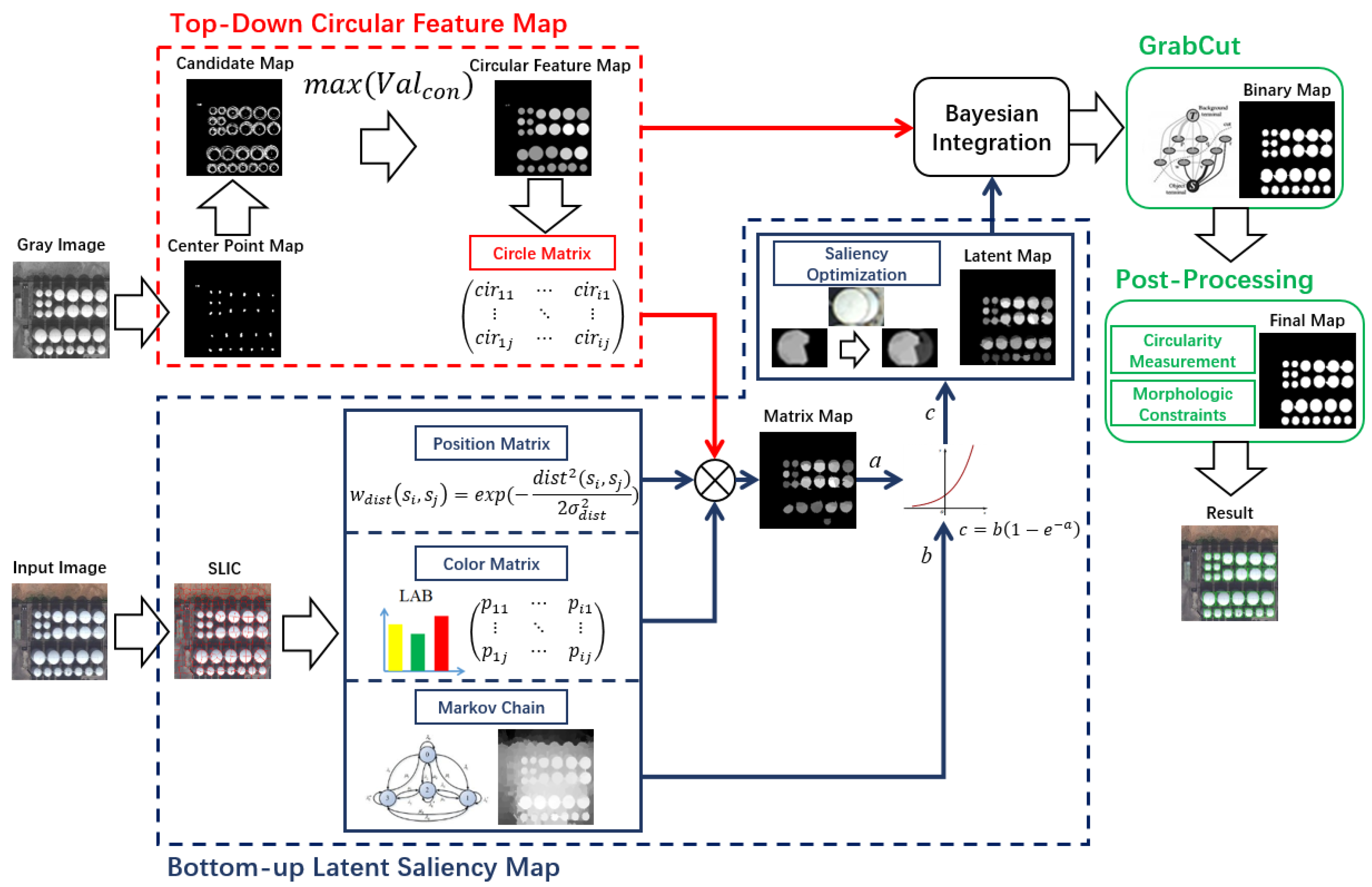
As shown in Figure 1, the US-CMC model is mainly divided into the following steps. Firstly, we use the SLIC [30] method to segment the image into super-pixels, and then we use a Color Markov Chain to obtain a coarse saliency region. Then we calculate the color and position matrix of super-pixel blocks and use them to obtain the saliency image. Secondly, we use the radial symmetry method to get information about the circular shapes in the image. Thirdly, The final grayscale image is obtained by Bayesian integration. Finally, the binary detection result is obtained by GrabCut and post-processing. Next, we will introduce each step in subsections.
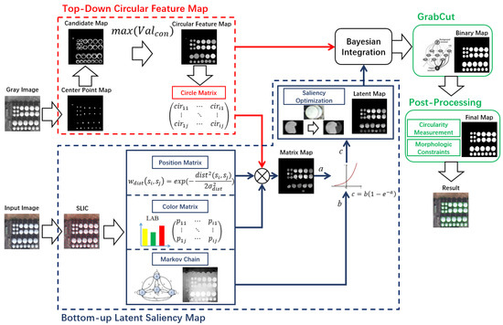
Figure 1.
Flowchart of the unsupervised saliency model with Color Markov Chain (US-CMC) method. First, a bottom-up latent saliency model combined with a circle matrix was applied to get the latent map. At the same time, the radial symmetry method was used to get the circular feature map then combine both maps by using Bayesian integration. Then, after One Cut for GrabCut and post-processing, the final result was obtained.
Because oil tanks are distributed targets, just like the absorption nodes in the Absorbing Markov Chain, each oil tank can be regarded as an absorbed node, and the super-pixels along the image side are regarded as the start nodes to absorb the entire super-pixels. Thus, we use Absorbing Markov Chain to help us with oil tank detection. a Markov chain is a relatively common and familiar random process. A Markov chain containing an absorption state is called an Absorbing Markov Chain. Given a series of data , the process starts from one of these states and moves continuously from one state to another. If the chain is currently in state , the probability of moving to state is called the transition probability, represented by . Therefore, the Markov chain can be determined by the transfer matrix P. For any Absorbing Markov Chain with k absorption states and m transient states, the canonical form of the above transition matrix P can be obtained as follows:
where Q is the probability transfer matrix of the transient state, the element in R means the transition probability between the transition and the absorption state, and I is the identity matrix of . We can get another matrix based on the matrix Q:
The element in N gives the expected number of times that the process changes to the transient state if it starts at the transient state . The final absorption probability matrix is as follows:
In the past, the saliency model based on an Absorbing Markov Chain used the absorption time to determine the saliency value. What we propose is a Color Markov Chain model that judges the saliency value based on the contrast of the image in CIE Lab color. The Color Markov Chain is a random walk model that is used to detect saliency regions in the image. Due to the segment representation by the super-pixel method, we can identify the image as . The vertex V is represented by a super-pixel, and E is a set of undirected edges containing the connectivity between two super-pixels. The edge connecting the two nodes i and j is denoted as , and represents the weight of the edge based on the similarity between the features defined on the nodes i and j. We use the CIE Lab color space to define the color characteristics of each super-pixel node because the CIE Lab color model describes how the color is displayed based on a human’s perception of color. The weight relationship expression between adjacent nodes i and j is:
We take all three channels of the CIE Lab color in the super-pixel block as the feature quantity of the two nodes i and j, which are represented by and , and , where , , and are the values of three channels in . , , and are the values of three channels in . The super-pixel result is shown in Figure 2b. is a constant used to control the weight; generally we set to 0.05. Then we get the affinity matrix of the undirected graph . Then we use the edge of the selected image as the absorption node to start the absorb process. At the same time, another affinity matrix between the transient node i and the absorption node j is established, where represents the correlation between nodes i and j in the image. . The is the same as in (4). We find the final correlation matrix , where . Then make , . The final absorption probability matrix B is obtained according to the above formula. Then define the saliency of each node as the dissimilarity with the image boundary. For the transient state in the Color Markov Chain, the probability absorbed by the absorption state actually represents the relationship between them. For each node i in the image, we sort the absorption probability values of all boundary nodes in the image boundary in descending order:

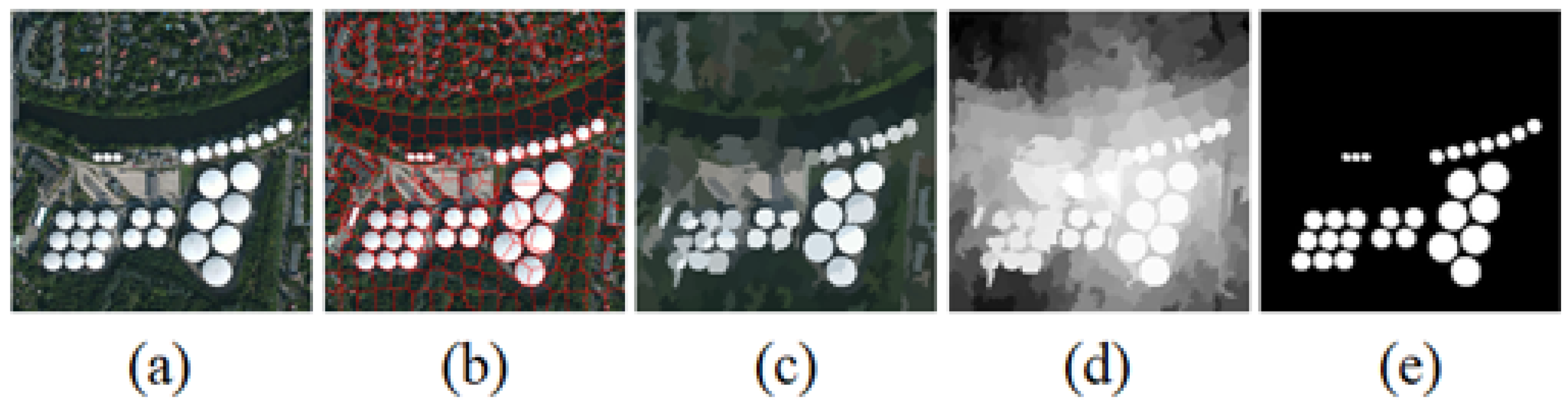
Figure 2.
An example of the process of a Color Markov Chain. (a) is the input image, (b) is the super-pixel segmentation, (c) is the result after averaging, (d) is the result of the Color Markov Chain, and (e) is the ground truth.
We take the first r column of , r is the number of columns in (where ), which is to represent the similarity between node i and the boundary node. And we present as the dissimilarity between node i and boundary nodes. So we get the final saliency value for each node:
In this way, we get a coarse saliency map based on the Color Markov Chain, which is the foreground probability distribution map. The results are shown in Figure 2d. Although it is not very accurate, it suppresses most of the background from the map. It also removes some of the shadow interference. Next we will use the color, position, and shape information of the map to construct a function to extract the features and then will highlight the salient areas we are really interested in.
When the image is divided by super-pixel, the image is labeled as , where n represents the number of super-pixels. In the previous process of the Color Markov Chain, we have formed an undirected graph , so that we can calculate the Euclidean distance of each super-pixel in the CIE Lab color space as the weight value of the edges. We define it as . Then, the Euclidean distance between the center points of the super-pixel blocks and is obtained, and the weight formula of the Euclidean distance is proposed:
We set to 0.25 according to the convention. Finally, we can get the contrast determination formula between two super-pixel blocks:
where is the circle matrix, which is the Euclidean distance of the average gray value in a super-pixel block between the super-pixels and in the circular feature map. The Formula (8) is also the basic formula for contrast optimization of the Color Markov Chain. In this paper, considering the characteristics of remote sensing object detection and the shape characteristics of the oil tank, we should also combine shape features for processing when we optimize the contrast of the Color Markov Chain. For shape features, we extract the circular features by calculating the radial symmetry of the gradients in the image. The method of radial symmetry will be explained in the next section. We integrate the result of the contrast determination formula into the Color Markov Chain as follows:
where is the Euclidean distance of saliency values between each super-pixel block in . Then we sum to get the saliency value of each super-pixel block itself:
The relevant results are shown in Figure 3c. The calculation of the saliency map in the above formula simply uses the method of multiplication and weighted summation, combining various low-level features and clues, and then optimizes the results of the Color Markov Chain. However, this kind of optimization is not enough, obviously. Through experiments, we find that some of the background areas are still not removed. Furthermore, we will optimize the results of the saliency map.

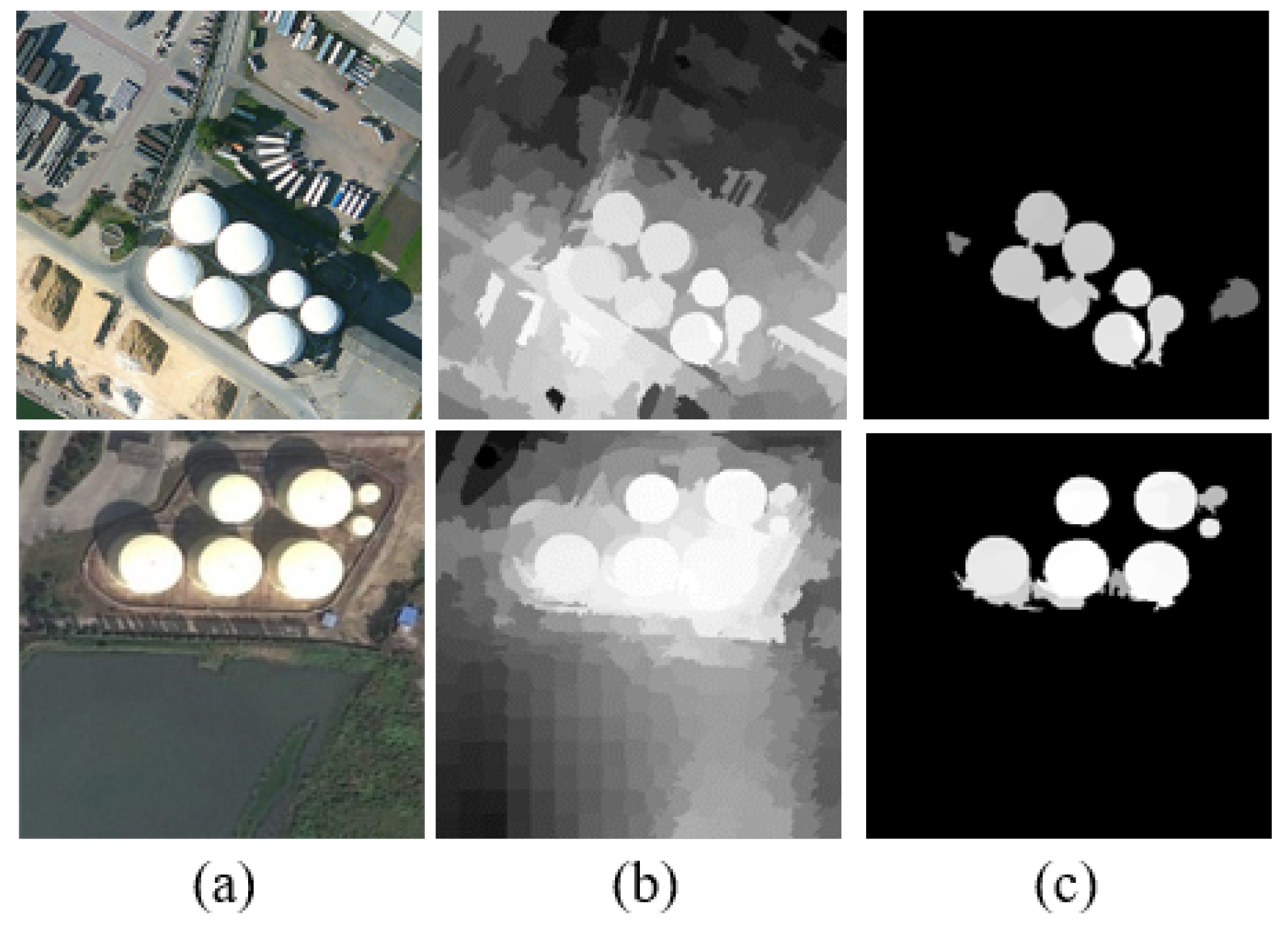
Figure 3.
(a) is the input image, (b) is the result of Color Markov Chain, and (c) is the result after contrast constraint.
2.2. Saliency Map Optimization and Background Suppression
Since the background of the original input image is very complicated, there is a significant disadvantage in some saliency maps where the background of the saliency map is not sufficiently suppressed. To solve this problem, we propose the following two methods. First, we group the nodes of the input image into K clusters by a K-means clustering algorithm in the CIE Lab color space, and then the saliency of each node can be corrected by simple interpolation of nodes in the same cluster. The saliency optimization of the node can be implemented by the following formula:
where m is the number of nodes in the cluster. , and is the sum of the variances in each feature dimension of the CIE Lab space. The term on the left side of Equation (11) represents the saliency of the initial optimization of the node , while the and on the right side of the formula are the original saliency results of the nodes and , respectively. The above parameter is set to 0.5 according to experience.
Although the above interpolation method effectively highlights the foreground of some saliency maps, some parts are still not well suppressed. To further solve this problem, we introduce a simple piecewise function to remove the part that is not saliency, or large, error regions. The function is defined as:
where is the threshold that defines the saliency range, set to 0.6 according to experience, and is the super-pixel. This way we get the final image of the latent map, as shown in Figure 4c.
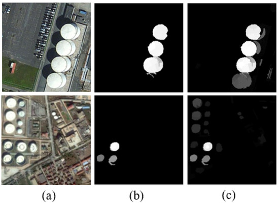
Figure 4.
(a) is the input image, (b) is the result after the above saliency model, and (c) is the latent map.
2.3. Top-Down Circular Feature Map Based on Circular Confidence Value
Oil tanks are often constructed of metal and are cylindrical in shape. In RSIs, the shape of the oil tank often appears round. Therefore, the result of target detection can be obtained by detecting circle areas in the image. However, the satellite may be at a certain angle to the surface of the earth. Especially in some areas with high latitudes, the final result of detection is probably not a regular circle. Therefore, the traditional Hough transform circle detection method is not able to detect most of the oil tanks that appear and even has a large number of misdetection problems. Aiming at this problem, we propose a circle detection method based on improved fast radial symmetric transformation, which can be applied to the above situation and has strong robustness. Though target detection only based on shape is not enough, it gives us a new way to think about the problem. The process is as follows:
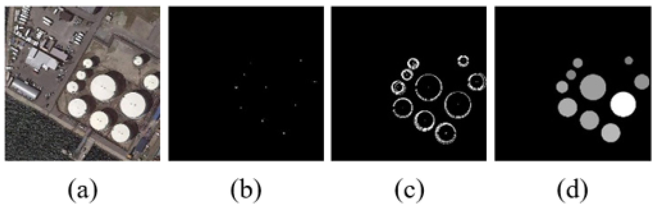
Given a radius interval R, let the radius of oil tank . Then, after obtaining the gradient of the image using Sobel transform, we can get the magnitude, which is called the “impact”, caused by a series of radii r and also calculate the direction of the gradient to determine whether the radius “fits” the gradient to form a circle. In theory, if the pixel is located just at the boundary of the circle with radius , then at , the effect of these pixels will be enriched at the center of the circle so that the approximate center position can be obtained. We can get the confidence value of each center point by adding all the magnitudes together. Then we find the point with and use this point as a center to form a circle with as its radius. We set the confidence value of the center as the gray value of the entire circle after being normalized. Then we can obtain the average distance between the super-pixels and in the circular feature map. Figure 5 shows the circular feature map generation process.
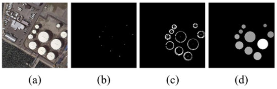
Figure 5.
(a) is the input image, (b) is the center point map, (c) is the candidate map, and (d) is the final circular feature map.
2.4. Fusion of Color Saliency Map and Circular Feature Map
After extracting the shape and color features of the target, we need to integrate these two different modules to achieve a better result. Therefore, we introduce a Bayesian integration function to fuse the results of the above two modules.
We set the latent map to and the result of the circular feature map to . We first define one of the pictures as the foreground map and the other picture as the background map. We calculate the possibilities of both so that we can integrate more information from different saliency maps. First, we use the average gray value of the image as the threshold and then we divide the graph by it. The images are divided into and , respectively, where is the foreground area and is the background area. In each region, we calculate the likelihood by comparing the foreground and background regions of and at pixel z. The formula is as follows:
where is the number of nonzero pixels of the foreground region in the image i, and represents the number of pixels whose saliency regions fall into the foreground bin , which contains . Similarly, represents the number of pixels of the background area i. The formula for calculating the posterior probability using is:
We can also use the formula in (16) to get another posterior probability using .
We then use these two posterior probabilities to calculate the final saliency map, which is as follows:
We should notice that Bayesian integration enforces the two graphs as prior and they cooperate with each other in an efficient manner; then the final result uniformly highlights the salient objects. So we add the two images together so that we can highlight the foreground of the two images at the same time. But the final result we need to get is a binary map. In the current situation, it is difficult to find a suitable threshold to convert the final saliency map into a binary map. The idea of setting a fixed threshold is too simple and easy to get false detections. So we introduce the One Cut for GrabCut [31] method to implement the binarization process. It is an improved version of GraphCut that sets an energy minimization function to calculate the threshold in each image, while also considering the completeness of the segmentation results. Minimized energy can be obtained by the following formula:
where is the saliency map we get, and refers to the saliency value of pixel z. indicates whether this pixel belongs to the foreground, 1 means the foreground, and 0 means the background. is the background and foreground overlap penalty, and are histograms inside object S and background , respectively, and is a smooth term. With One Cut, we can get the binarized form of each map.
2.5. Post-Processing
The post-processing part was introduced because we have obtained the binary map results for the oil tank area, but the result we need to get is a more accurate one. Because Grabcut brings problems such as some small noises, we extract the area information and shape information from all of the noises separately and compare it with the area of the oil tank, then propose a method to remove the noise. We first remove the regions with less than 40 pixels and then solve the circularity for all the remaining connected domain. The circularity formula is as follows:
where is the area of the connected domain i, and is the perimeter of it. Then we will get the circularity and can remove all the parts that do not conform to the circle, and the remaining regions we see as the final oil tank area, so we get the final result.
3. Experimental Results And Discussion
We created a dataset for detection that is comprised of a total of 240 multi-resolution images from Google Earth. The resolution of the test images is . All test images contain at least two or more oil tanks for testing. The full dataset has a total of more than 2200 oil tanks of various colors and luminances. The scales of the oil tanks are from 7 m to 40 m. In addition, we manually mark all of the ground truth to ensure that the ground truth fits perfectly with the oil tank area. At the same time, in order to make the detection task more difficult, we also added nearly 35 test images with similar color and shape interferences for detection. Here is our experiment:
3.1. Parameter Selection
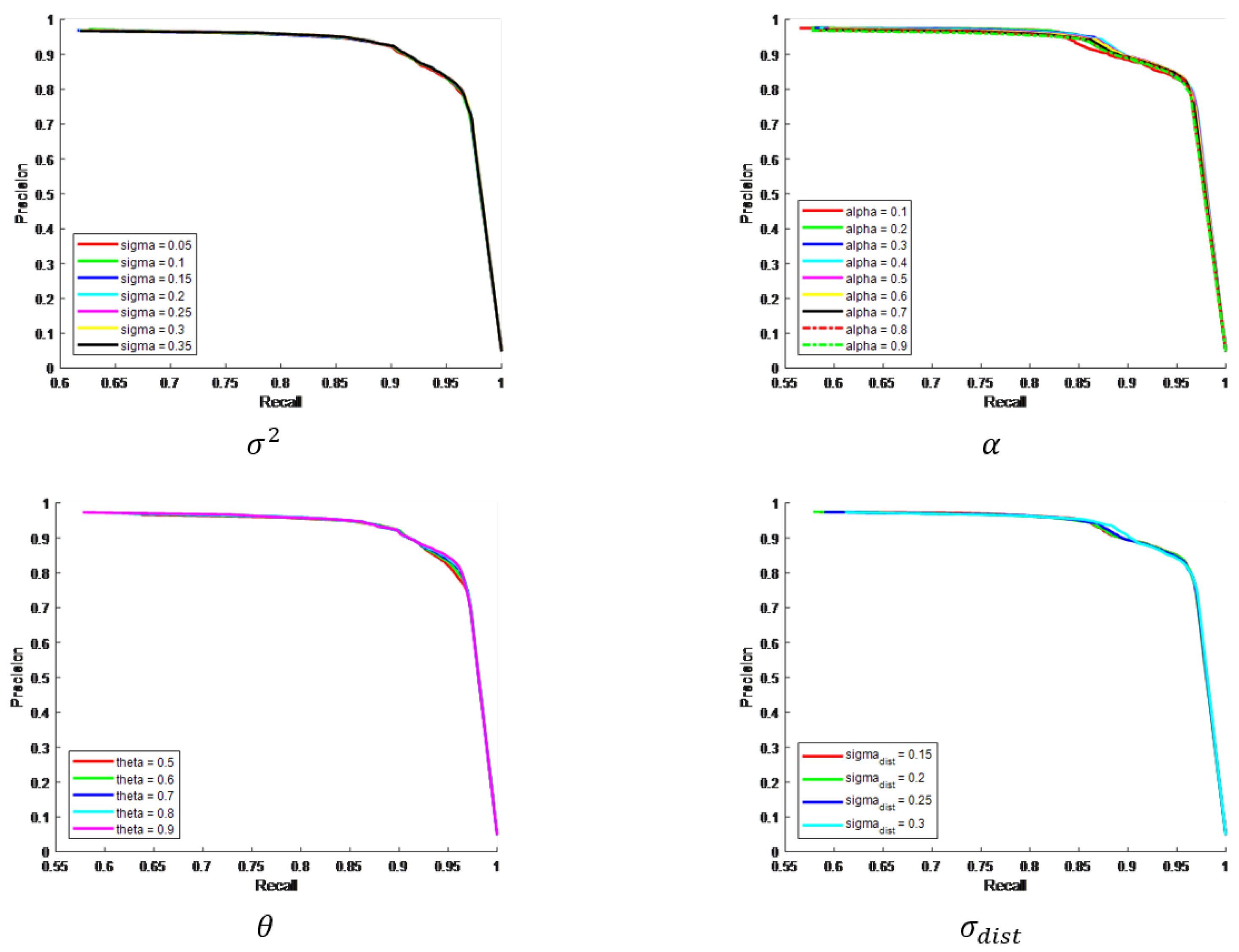
Before comparing the saliency models and oil tank detection methods, we need to use experiments to verify the parameters. For all of the parameters such as , , , and in our text, we supplanted the parameter analysis through a P–R curve to verify the performance of each parameter on our results. As shown in Figure 6, the change of four parameters does not have a significant effect on the P–R curve. Therefore, these four parameter selections are appropriate.
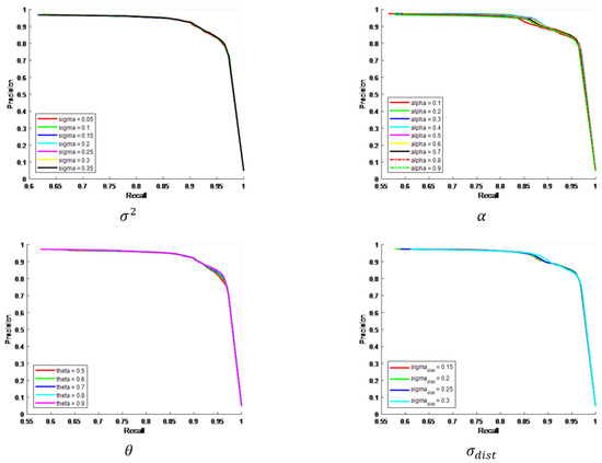
Figure 6.
The P–R curve result of four parameters.
3.2. Comparison with Saliency Models
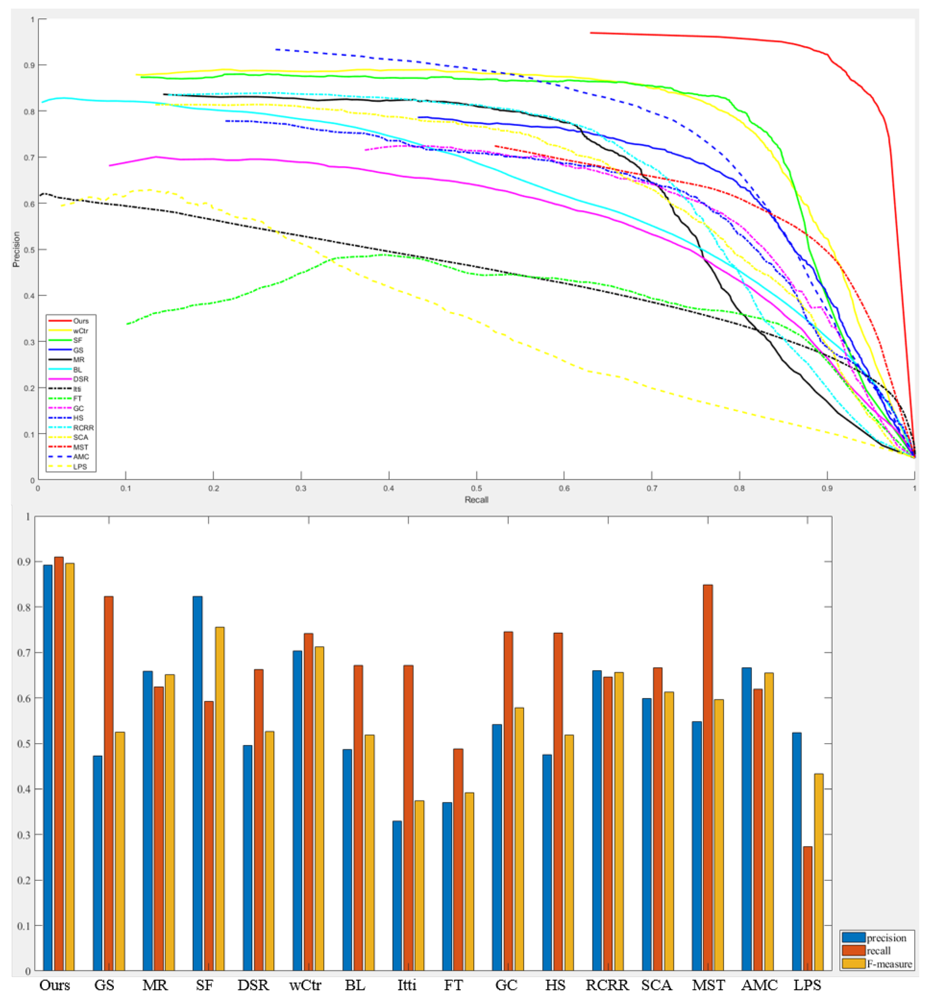
In order to highlight the superiority of our method, we first compare the US-CMC model with 15 currently advanced saliency models, namely wCtr [22], SF [20], GS [24], MR [23], BL [26], DSR [21], FT [17], GC [32], HS [33], RCRR [34], AMC [35], MST [25], LPS [36], SCA [27], Itti [15]. We will use three indicators, mean absolute error(MAE), precision–recall curve(P–R Curve), and F-measure to evaluate the advantages and disadvantages of each model. The mean absolute error formula and the F-measure formula are as follows:
When the test results are evaluated using the F-Measure in this paper, the value of is set to 0.3. Since the P–R curve needs to ensure that the final image is a grayscale image, we compare the results with other saliency models.
As shown in Table 1, Figure 7 and Figure 8, our model is the best of all the saliency detection models and far better than all of the others. This is mainly due to the following reasons: Firstly, previous saliency models are generally designed to solve the problem of natural images. For RSIs, due to their complex background information, saliency models can only judge whether the region is salient by relying on the color information and the position of the parts of interest in the image. Although the color of the oil tank is mostly light, it is still easy to misjudge just according to color information because other light-colored natural objects or buildings are also regarded as oil tanks. At the same time, it is difficult to accurately identify the oil tank because of the similarity in color and texture between oil tank and background. Since it combines a bottom-up low-level feature with a top-down circular feature map, the US-CMC model can be more accurate in identifying the oil tank target. Therefore, our model has better detection performance for oil tanks than the traditional saliency models.

Table 1.
The MAE result.
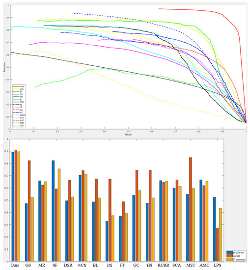
Figure 7.
The result of the P–R curve and F-measure in the experiment.
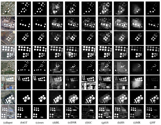
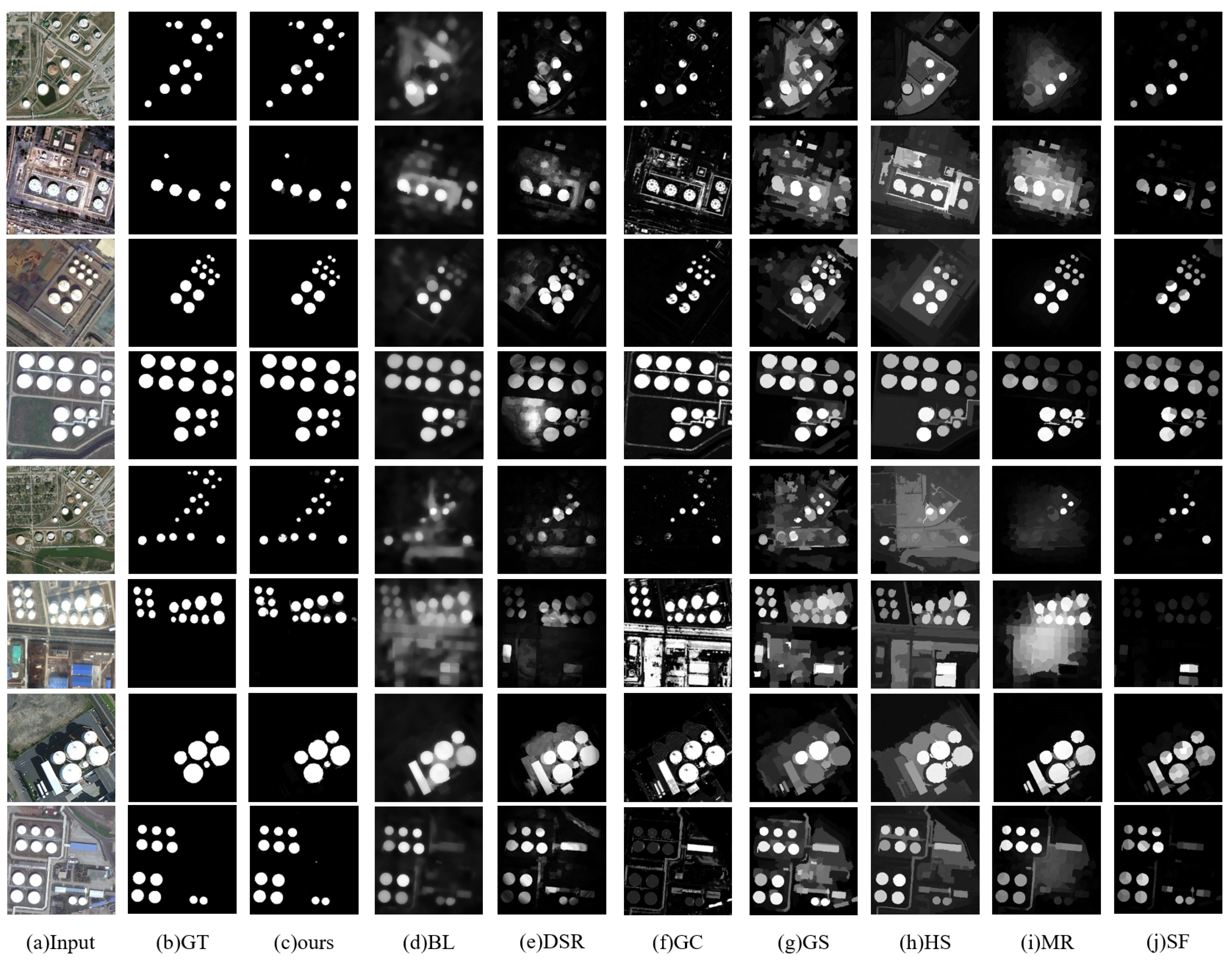
Figure 8.
Comparison of results with other saliency models.
3.3. Comparison with Oil Tank Detection Methods
After comparing it with the saliency detection models, in order to verify the effectiveness of our proposed method, we also need to compare it with the current advanced oil tank detection methods. We compare two different methods of oil tank detection. The first [10] is a supervised algorithm combined with CNN feature extractor and SVM classifier, and the other [7] is an oil tank detection method based entirely on geographic shape information. We randomly select 190 of the 240 images to train the CNN network, and then use the remaining images to compare the effects of the three oil tank detection methods. To evaluate the test results, we define the result of true positives when the Intersection over Union(IoU) value is greater than 0.7 and define false positives as the result of IoU values less than 0.3. This will prevent some unsuccessfully detected oil tanks from being labeled with both false and missed inspections. The test results are shown in Table 2.
Table 2.
IoU test results for three oil tank detection methods.
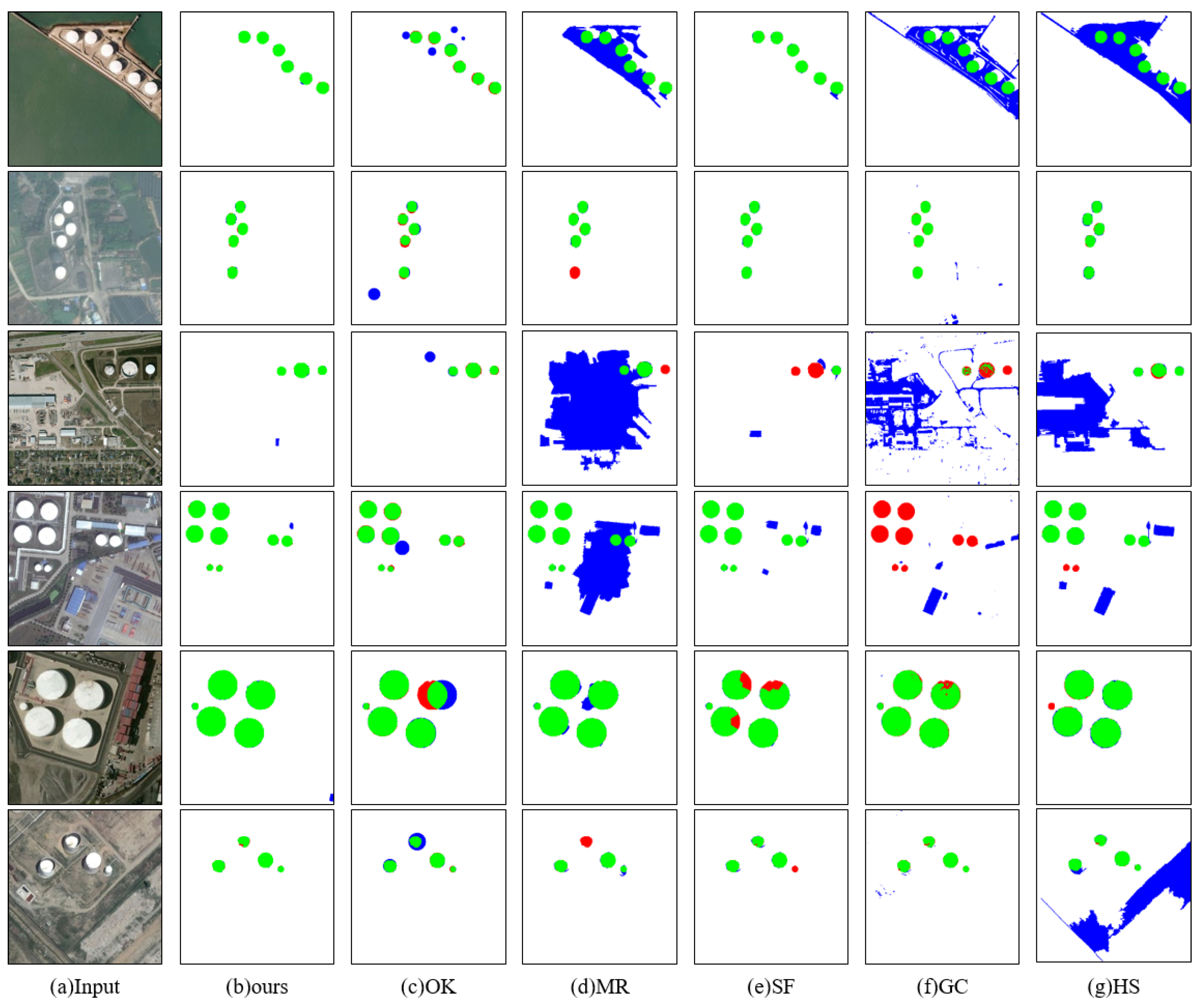
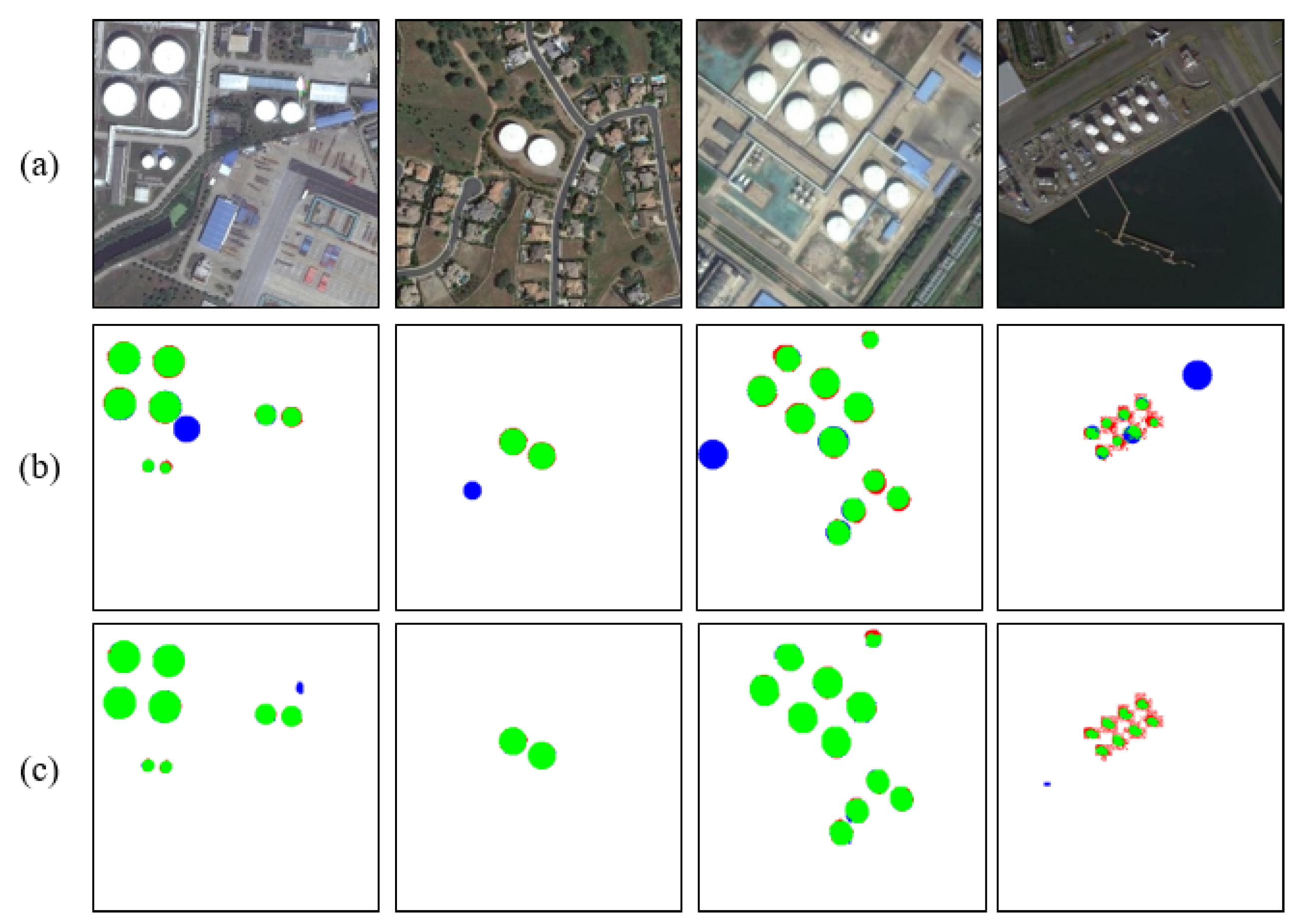
In Table 2, we can see that our method is the best in terms of both the precision rate and the recall rate compared with the other state-of-art detection methods. Although Zhang’s method combines feature extraction and supervised learning with CNN, it requires a large dataset as training set, which undoubtedly consumes human and material resources for marking ground truth and lacks efficiency. In the face of a small training dataset, there is no superiority of the supervised algorithm. The excellent performance of our method shows that even without effective learning, there are still very good performances. As shown in Figure 9c, Ok’s method relies only on the circle shape information obtained from the gradient of the image. It has its own limitations. When the oil tank has a circular shadow, or other non-oil tank areas have a circular gradient, it is easy to lead to false detection. At the same time, many external factors such as illumination will change the gradient of the oil tank contour, and because of its lack of guidance and assistance from other features, they always misjudge the actual size of the oil tank, resulting in false detection results.
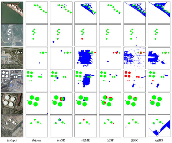
Figure 9.
Comparison of final test results. Green is the positive detection area, blue is the false detection area, and red is the missed detection area.
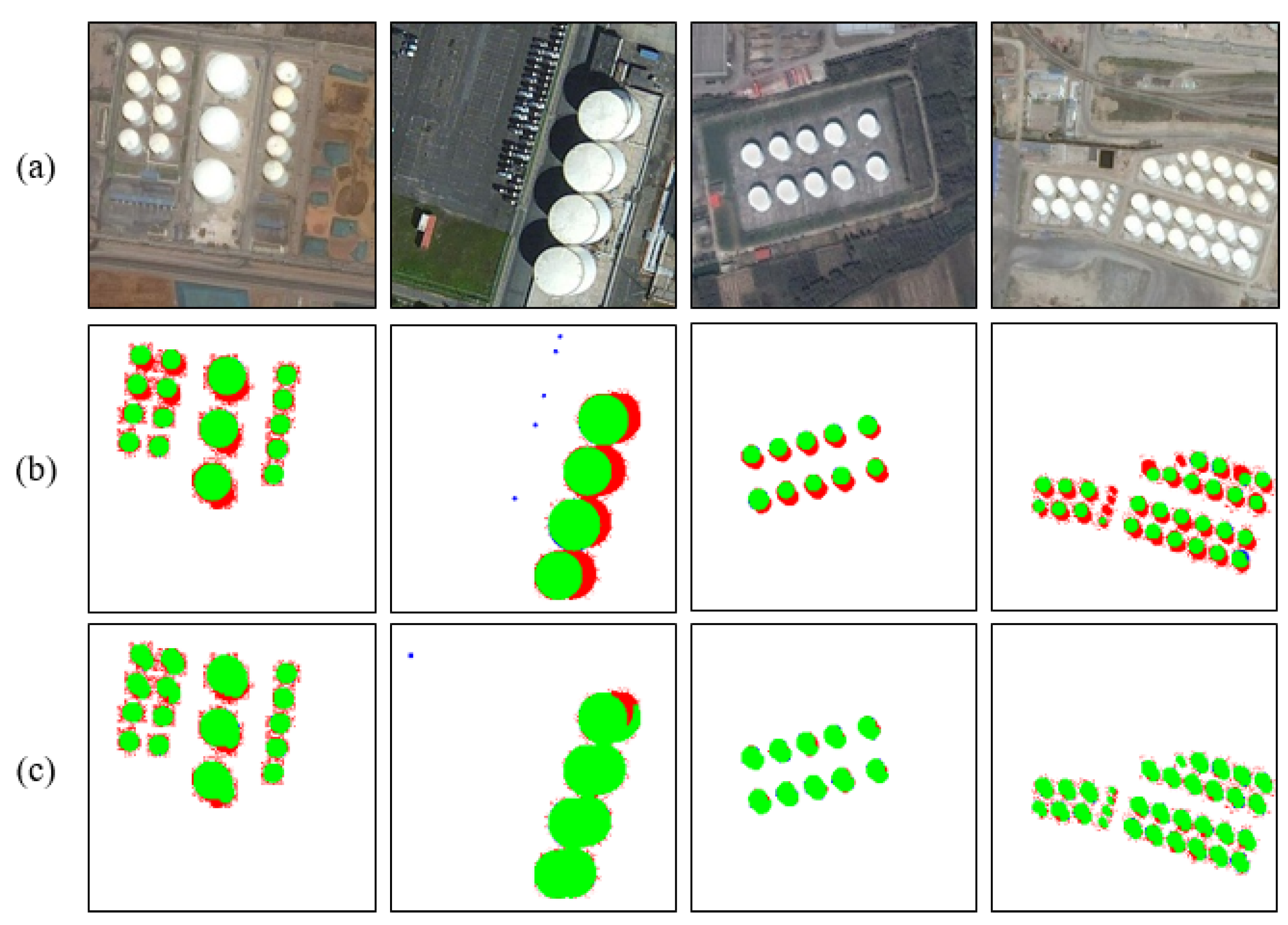
Compared with the radial symmetry detection method separately, we find that our method performs better than the radial oil tank detection method proposed by Ok in the following three cases. Figure 10, Figure 11 and Figure 12 show that our method can overcome these influences well when the oil tank is at a certain angle, or when there are certain non-tank circular zone disturbances and shadow problems caused by the sunlight.

Figure 10.
Comparison of two detection methods when the oil tank is at a certain angle. (a) is the input image, (b) is the method from Ok, (c) is our method.
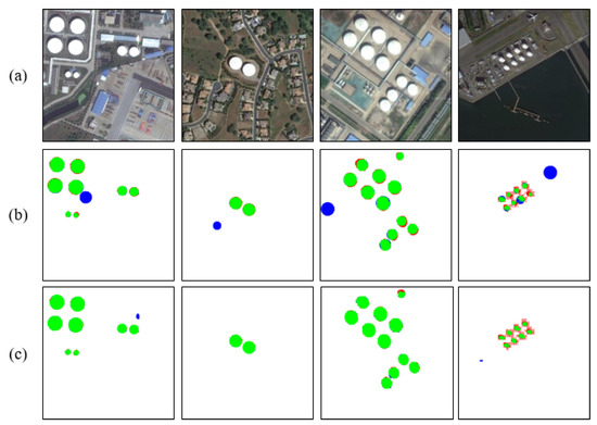
Figure 11.
Comparison of two detection methods when similar shapes occur. (a) is the input image, (b) is the method from Ok, (c) is our method.
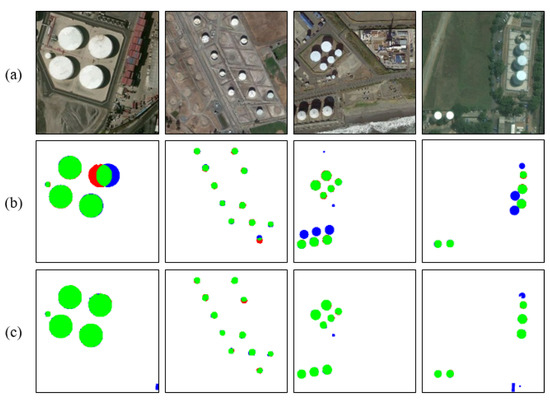
Figure 12.
Comparison of two detection methods when shadow interference occurs. (a) is the input image, (b) is the method from Ok, (c) is our method.
Firstly, our method is based on a US-CMC model. In the process of the Color Markov Chain, due to the color difference with the main part of the oil tank and the similarity with the background, shadows are more easily absorbed. Therefore, the saliency value of a shadow is generally low, while the saliency value of an oil tank’s body is relatively high. With further color constraints, the shadow has been largely eliminated. So this method is robust to the presence of shadows. At the same time, when the oil tank is at a certain angle to the satellite, according to Figure 10, we can see that the body part of the oil tank can be detected well after color interpolation. Therefore, even if the oil tank has a certain angle due to the latitude of the Earth, the oil tank can still be detected completely, while using only one single feature such as the circle is unachievable. Finally, when similar shapes occur, as shown in the second column of Figure 11, there is a roundabout in the input image, which is identified as the oil tank by Ok’s method. However, our method determines this area to be background by comparing with the surrounding area. The input image in the fourth column has an incomplete ring next to the oil tank, which is identified as a true target by Ok’s method. It is obvious that there are great limitations in oil tank detection by relying only on shape detection. Our method can solve such limitations and improve the accuracy of the whole process of detection.
3.4. Robustness for Our Methods
In this section, we will show that our method is good not only when the oil tank is at a certain angle, or has certain non-tank circular zone disturbances and shadow problems caused by the sunlight, but also has excellent results when oil tanks are in misty and dusty condition, as well as in higher resolution visible light remote sensing images.
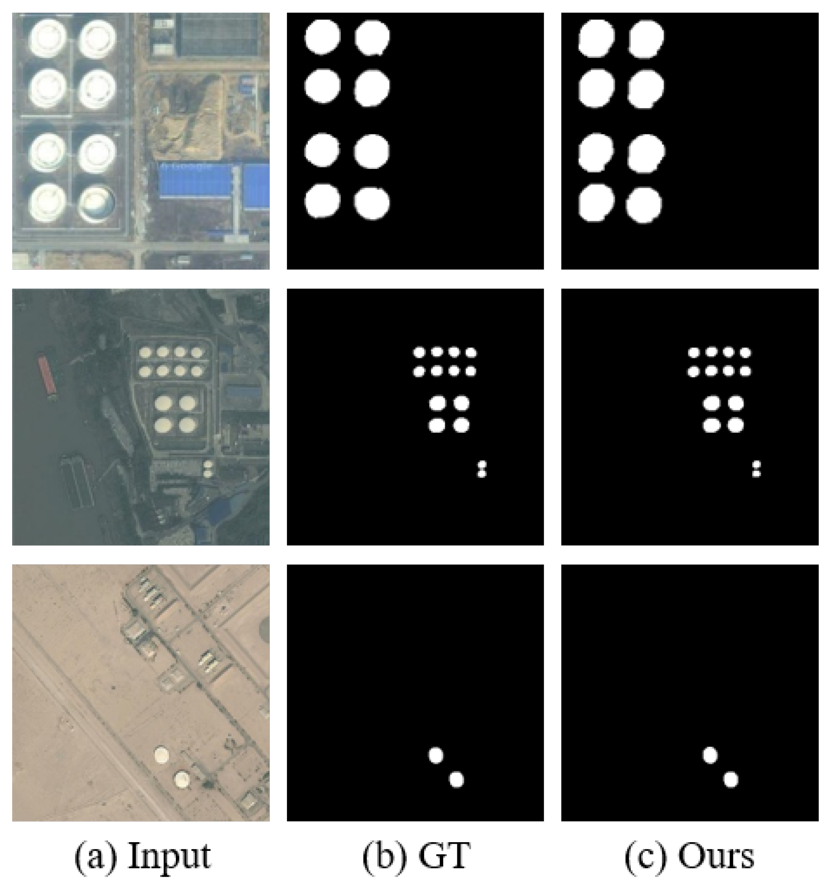
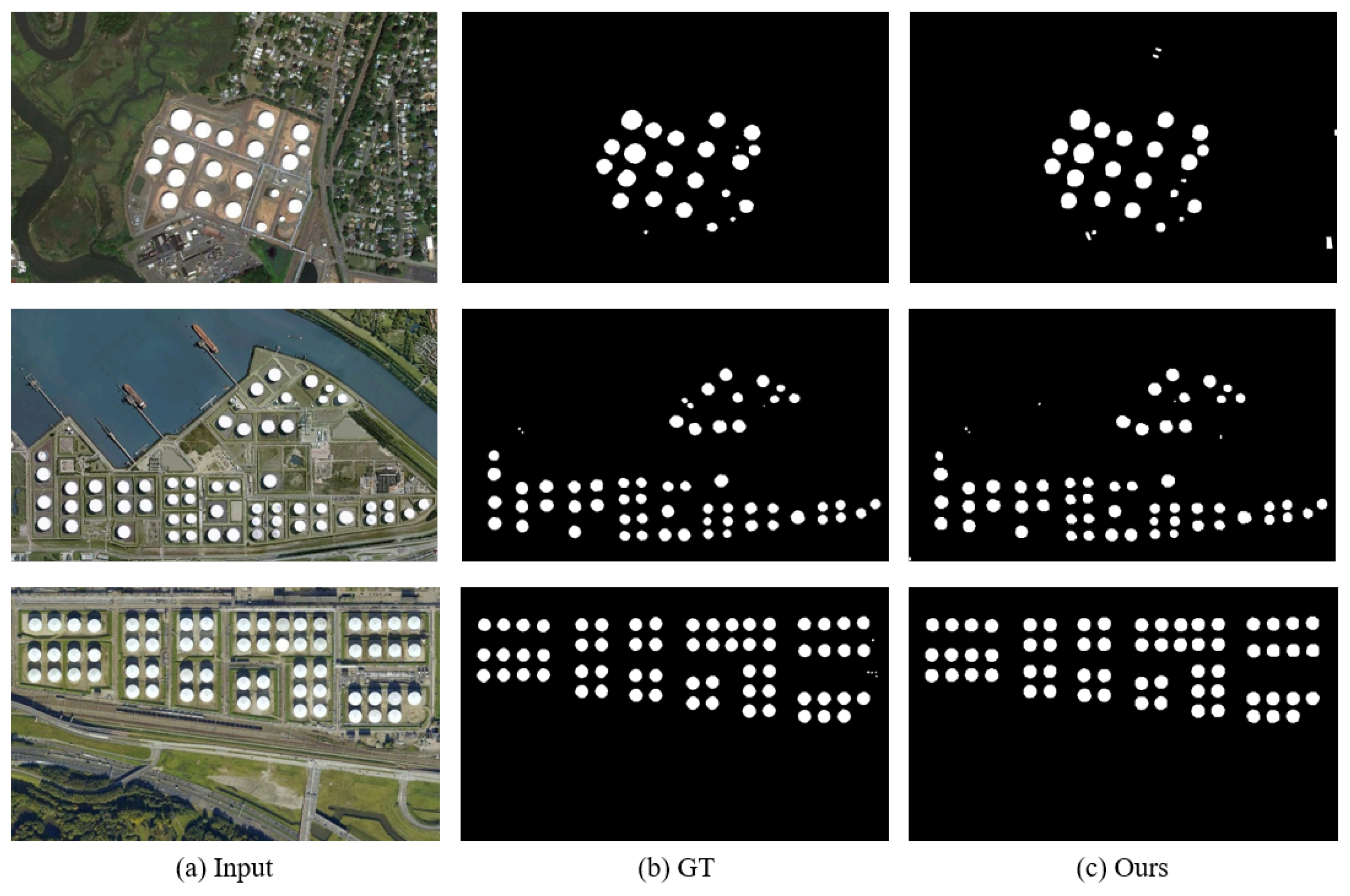
The principle of our algorithm is based on color, gradient, and shape information so that the target existing in the image can be detected. In addition to against disturbances caused by shadows and sensor inclination angle, our method also works well in misty and dusty environments. From the result shown in Figure 13, it can be seen that our method is also excellent. In terms of high resolution, our method can also achieve better results and is robust in high-resolution remote sensing images. The results can be seen in Figure 14. The input images in Figure 14 are all four times bigger than the images in the test dataset.
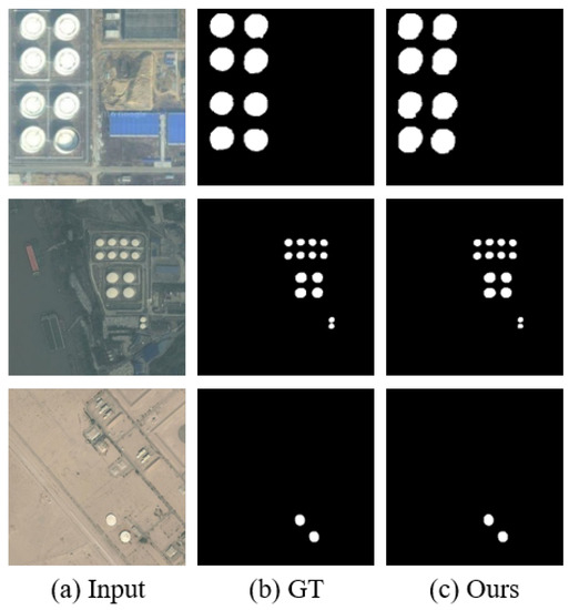
Figure 13.
Our method works in misty and dusty condition. (a) is the input image, (b) is the ground truth, (c) is our method.
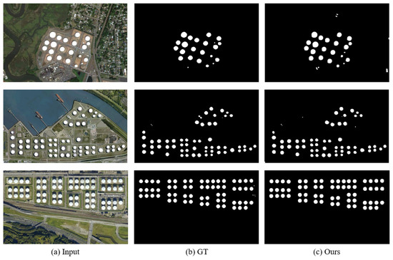
Figure 14.
Our methods works in high resolution images. (a) is the input image, (b) is the ground truth, (c) is our method.
4. Conclusions
According to the characteristics of oil tanks in RSIs, in this paper, we propose an unsupervised oil tank detection method that takes advantage of low-level saliency to highlight latent target areas and introduce a circular feature map to the saliency model to suppress the background. Compared with other saliency models, our model is designed for oil tanks, and can better eliminate the interference of color and texture in similar areas. Our method is also simpler and faster than the learning-based detection method because it does not need sample collection or a training process. Compared with the geometry-based detection method, we incorporate shape information into the saliency model, both using color features to extract the potential target regions and shape information to eliminate the interference of similar regions. Consequently, the US-CMC has outstanding performance in terms of precision rate and recall rate under the conditions with shadows, view angle, and shape interference. Next, we plan to apply the Markov chain to higher-resolution remote sensing images and try to use shape information to absorb and reconstruct the super-pixel blocks in order to obtain better results.
Author Contributions
Z.L. designed and implemented the whole detection model and drafted the manuscript. D.Z. proposed the direction of research and designed the experiment. Z.S. and Z.J. reviewed and edited the manuscript.
Funding
This research was supported by the National Key R&D Program of China under Grant 2017YFC 1405600, the National Natural Science Foundation of China under Grant 61671037, and the Aeronautical Science Foundation of China under Grant 2017ZC51046.
Acknowledgments
The authors would like to thank the editors and anonymous reviewers for their valuable comments, which are very helpful in revising this paper.
Conflicts of Interest
The authors declare no conflict of interest.
References
- Xu, H.; Chen, W.; Sun, B.; Chen, Y.; Li, C. Oil tank detection in synthetic aperture radar images based on quasi-circular shadow and highlighting arcs. J. Appl. Remote Sens. 2014, 8, 397–398. [Google Scholar] [CrossRef]
- Zhang, W.; Hong, Z.; Chao, W.; Tao, W. Automatic oil tank detection algorithm based on remote sensing image fusion. In Proceedings of the IEEE International Geoscience and Remote Sensing Symposium (IGARSS), Seoul, Korea, 25–29 July 2005; pp. 3956–3958. [Google Scholar]
- Atherton, T.J.; Kerbyson, D.J. Size invariant circle detection. Image Vis. Comput. 1999, 17, 795–803. [Google Scholar] [CrossRef]
- Li, B.; Yin, D.; Yuan, X.; Li, G. Oilcan recognition method based on improved Hough transform. Opto-Electron. Eng. 2008, 35, 30–44. [Google Scholar]
- Han, X.; Fu, Y.; Li, G. Oil depots recognition based on improved Hough transform and graph search. J. Electron. Inf. Technol. 2011, 33, 66–72. [Google Scholar] [CrossRef]
- Zhu, C.; Liu, B.; Zhou, Y.; Yu, Q.; Liu, X.; Yu, W. Framework design and implementation for oil tank detection in optical satellite imagery. In Proceedings of the IEEE International Geoscience and Remote Sensing Symposium (IGARSS), Munich, Germany, 22–27 July 2012; pp. 6016–6019. [Google Scholar]
- Ok, A.O.; Baseski, E. Circular oil tank detection from panchromatic satellite images: A new automated approach. IEEE Geosci. Remote Sens. Lett. 2015, 12, 1347–1351. [Google Scholar] [CrossRef]
- Cai, X.; Sui, H.; Lv, R.; Song, Z. Automatic circular oil tank detection in high-resolution optical image based on visual saliency and hough transform. In Proceedings of the 2014 IEEE Workshop on Electronics, Computer and Applications(IWECA), Ottawa, ON, Canada, 8–9 May 2014; pp. 408–411. [Google Scholar]
- Yao, Y.; Jiang, Z.; Zhang, H. Oil tank detection based on salient region and geometric features. In Proceedings of the SPIE/COS Photonics Asia, Beijing, China, 9 October 2014. [Google Scholar]
- Zhang, L.; Shi, Z.; Wu, J. A hierarchical oil tank detector with deep surrounding features for high-resolution optical satellite imagery. IEEE J. Sel. Top. Appl. Earth Obs. Remote Sens. 2015, 8, 4895–4909. [Google Scholar] [CrossRef]
- Wang, Q.; Zhang, J.; Hu, X.; Wang, Y. Automatic Detection and Classification of Oil Tanks in Optical Satellite Images Based on Convolutional Neural Network. In Proceedings of the International Conference on Image and Signal Processing(ICISP), Trois-Rivières, QC, Canada, 30 May–1 June 2016; pp. 304–313. [Google Scholar]
- Cheng, G.; Zhou, P.; Han, J. Learning rotation-invariant convolutional neural networks for object detection in vhr optical remote sensing images. IEEE Trans. Geosci. Remote Sens. 2016, 54, 7405–7415. [Google Scholar] [CrossRef]
- Duda, R.O.; Hart, P.E. Use of the Hough transformation to detect lines and curves in pictures. Commun. ACM 1972, 15, 11–15. [Google Scholar] [CrossRef]
- Zhang, L.; Wang, S.; Liu, C.; Wang, Y. Saliency-Driven Oil Tank Detection Based on Multidimensional Feature Vector Clustering for SAR Images. IEEE Geosci. Remote Sens. Lett. 2014, 1–5. [Google Scholar] [CrossRef]
- Itti, L.; Koch, C.; Niebur, E. A model of saliency-based visual attention for rapid scene analysis. IEEE Trans. Pattern Anal. Mach. Intell. 1998, 20, 1254–1259. [Google Scholar] [CrossRef]
- Hou, X.; Zhang, L. Saliency detection: A spectral residual approach. In Proceedings of the IEEE Conference on Computer Vision and Pattern Recognition (CVPR), Minneapolis, MN, USA, 18–23 June 2007. [Google Scholar]
- Achanta, R.; Hemami, S.; Estrada, F.; Susstrunk, S. Frequency-tuned salient region detection. In Proceedings of the IEEE Conference on Computer Vision and Pattern Recognition (CVPR), Miami, FL, USA, 20–25 June 2009; pp. 1597–1604. [Google Scholar]
- Goferman, S.; Zelnik-Manor, L.; Tal, A. Context-aware saliency detection. In Proceedings of the IEEE Conference on Computer Vision and Pattern Recognition (CVPR), San Francisco, CA, USA, 13–18 June 2010; pp. 2376–2383. [Google Scholar]
- Cheng, M.; Zhang, G.; Mitra, N.J.; Huang, X.; Hu, S. Global contrast based salient region detection. In Proceedings of the IEEE Conference on Computer Vision and Pattern Recognition (CVPR), Colorado Springs, CO, USA, 20–25 June 2011; pp. 409–416. [Google Scholar]
- Perazzi, F.; Krahenbuhl, P.; Pritch, Y.; Hornung, A. Saliency filters: Contrast based filtering for salient region detection. In Proceedings of the IEEE Conference on Computer Vision and Pattern Recognition (CVPR), Providence, RI, USA, 16–21 June 2012; pp. 733–740. [Google Scholar]
- Lu, H.; Li, X.; Zhang, L.; Ruan, X.; Yang, M.H. Dense and sparse reconstruction error based saliency descriptor. IEEE Trans. Image Process. 2016, 25, 1592–1603. [Google Scholar] [CrossRef] [PubMed]
- Zhu, W.; Liang, S.; Wei, Y.; Sun, J. Saliency optimization from robust background detection. In Proceedings of the IEEE Conference on Computer Vision and Pattern Recognition (CVPR), Columbus, OH, USA, 23–28 June 2014; pp. 2814–2821. [Google Scholar]
- Yang, C.; Zhang, L.; Lu, H.; Ruan, X.; Yang, M.H. Saliency Detection via Graph-Based Manifold Ranking. In Proceedings of the IEEE International Conference on Computer Vision and Pattern Recognition (CVPR), Portland, OR, USA, 23–28 June 2013; pp. 3166–3173. [Google Scholar]
- Wei, Y.; Wen, F.; Zhu, W.; Sun, J. Geodesic Saliency Using Background Priors. In Proceedings of the European Conference on Computer Vision (ECCV), Florence, Italy, 7–13 October 2012; pp. 29–42. [Google Scholar]
- Tu, W.; He, S.; Yang, Q.; Chien, S. Real-Time Salient Object Detection with a Minimum Spanning Tree. In Proceedings of the IEEE Conference on Computer Vision and Pattern Recognition (CVPR), Las Vegas, NV, USA, 27–30 June 2016; pp. 2334–2342. [Google Scholar]
- Tong, N.; Lu, H.; Ruan, X.; Yang, M. Salient Object Detection via Bootstrap Learning. In Proceedings of the IEEE Conference on Computer Vision and Pattern Recognition (CVPR), Boston, MA, USA, 7–12 June 2015; pp. 1884–1892. [Google Scholar]
- Qin, Y.; Lu, H.; Xu, Y.; Wang, H. Saliency Detection via Cellular Automata. In Proceedings of the IEEE Conference on Computer Vision and Pattern Recognition (CVPR), Boston, MA, USA, 7–12 June 2015; pp. 110–119. [Google Scholar]
- Lee, G.; Tai, Y.; Kim, J. Deep Saliency with Encoded Low Level Distance Map and High Level Features. In Proceedings of the IEEE Conference on Computer Vision and Pattern Recognition (CVPR), Las Vegas, NV, USA, 27–30 June 2016; pp. 660–668. [Google Scholar]
- Wang, T.; Zhang, L.; Wang, S.; Lu, H.; Yang, G.; Ruan, X.; Borji, A. Detect Globally, Refine Locally: A Novel Approach to Saliency Detection. In Proceedings of the IEEE Conference on Computer Vision and Pattern Recognition (CVPR), Salt Lake City, UT, USA, 18–22 June 2018; pp. 4321–4329. [Google Scholar]
- Achanta, R.; Shaji, A.; Smith, K.; Lucchi, A.; Fua, P.; Süsstrunk, S. SLIC superpixels compared to state-of-the-art superpixel methods. IEEE Trans. Pattern Anal. Mach. Intell. 2012, 34, 2274–2282. [Google Scholar] [CrossRef] [PubMed]
- Tang, M.; Gorelick, L.; Veksler, O.; Boykov, Y. GrabCut in One Cut. In Proceedings of the IEEE International Conference on Computer Vision (ICCV), Sydney, Australia, 1–8 December 2013; pp. 1769–1776. [Google Scholar]
- Cheng, M.; Warrell, J.; Lin, W.; Zheng, S.; Vineet, V.; Crook, N. Efficient Salient Region Detection with Soft Image Abstraction. In Proceedings of the International Conference on Computer Vision (ICCV), Sydney, Australia, 1–8 December 2013; pp. 1529–1536. [Google Scholar]
- Yan, Q.; Xu, L.; Shi, J.; Jia, J. Hierarchical Saliency Detection. In Proceedings of the IEEE Conference on Computer Vision and Pattern Recognition (CVPR), Portland, OR, USA, 23–28 June 2013; pp. 1155–1162. [Google Scholar]
- Yuan, Y.; Li, C.; Kim, J.; Cai, W.; Feng, D.D. Reversion Correction and Regularized Random Walk Ranking for Saliency Detection. IEEE Trans. Image Process. 2018, 27, 1311–1322. [Google Scholar] [CrossRef] [PubMed]
- Sun, J.; Lu, H.; Liu, X. Saliency Region Detection Based on Markov Absorption Probabilities. IEEE Trans. Image Process. 2015, 24, 1639–1649. [Google Scholar] [CrossRef] [PubMed]
- Li, H.; Lu, H.; Lin, Z.; Shen, X.; Price, B. Inner and Inter Label Propagation: Salient Object Detection in the Wild. IEEE Trans. Image Process. 2015, 24, 3176–3186. [Google Scholar] [CrossRef] [PubMed]


© 2019 by the authors. Licensee MDPI, Basel, Switzerland. This article is an open access article distributed under the terms and conditions of the Creative Commons Attribution (CC BY) license (http://creativecommons.org/licenses/by/4.0/).