Article

Remote Sensing of Sea Surface Salinity: Comparison of Satellite and In Situ Observations and Impact of Retrieval Parameters

1
NASA Goddard Space Flight Center, Greenbelt, MD 20771, USA
2
Center of Excellence in Earth Systems Modeling & Observations (CEESMO), Chapman University, Orange, CA 92866, USA
3
Sorbonne Université, CNRS, IRD, MNHN, Laboratoire d’Océanographie et du Climat: Expérimentations et Approches Numériques (LOCEAN), 75005 Paris, France
4
Remote Sensing Systems, Santa Rosa, CA 95401, USA
5
Earth & Space Research, Seattle, WA 98121, USA
*
Author to whom correspondence should be addressed.
Remote Sens. 2019, 11(7), 750; https://doi.org/10.3390/rs11070750
Submission received: 14 February 2019 / Revised: 22 March 2019 / Accepted: 24 March 2019 / Published: 28 March 2019
(This article belongs to the Special Issue Sea Surface Salinity Remote Sensing)

Abstract

:
Since 2009, three low frequency microwave sensors have been launched into space with the capability of global monitoring of sea surface salinity (SSS). The European Space Agency’s (ESA’s) Microwave Imaging Radiometer using Aperture Synthesis (MIRAS), onboard the Soil Moisture and Ocean Salinity mission (SMOS), and National Aeronautics and Space Administration’s (NASA’s) Aquarius and Soil Moisture Active Passive mission (SMAP) use L-band radiometry to measure SSS. There are notable differences in the instrumental approaches, as well as in the retrieval algorithms. We compare the salinity retrieved from these three spaceborne sensors to in situ observations from the Argo network of drifting floats, and we analyze some possible causes for the differences. We present comparisons of the long-term global spatial distribution, the temporal variability for a set of regions of interest and statistical distributions. We analyze some of the possible causes for the differences between the various satellite SSS products by reprocessing the retrievals from Aquarius brightness temperatures changing the model for the sea water dielectric constant and the ancillary product for the sea surface temperature. We quantify the impact of these changes on the differences in SSS between Aquarius and SMOS. We also identify the impact of the corrections for atmospheric effects recently modified in the Aquarius SSS retrievals. All three satellites exhibit SSS errors with a strong dependence on sea surface temperature, but this dependence varies significantly with the sensor. We show that these differences are first and foremost due to the dielectric constant model, then to atmospheric corrections and to a lesser extent to the ancillary product of the sea surface temperature.

Graphical Abstract

1. Introduction

Sea surface salinity (SSS) is a key parameter for physical oceanography and the study of the hydrological cycle. Together with sea surface temperature (SST), it determines surface water density which impacts the vertical flow through the thermohaline component of the ocean circulation. SSS is also a tracer of the water cycle, because it is impacted by precipitations and evaporation, rivers outflow, and ice formation and melt. Until the early 2000’s, SSS had been observed sparsely, largely along commercial shipping lanes or during spatially or temporally limited oceanographic campaigns, resulting in spatial and temporal coverage inadequate for many applications. The sampling largely improved during the second half of the 2000’s due to the rapid expansion of the deployment of the Argo network of free drifting profiling floats. But the spatial and temporal coverage of in situ measurements cannot rival that of satellite observations which constitute a critical component of the ocean observation system. In this context, two satellite missions were launched with the objective of monitoring SSS at a global scale with weekly to monthly temporal resolution. In November 2009, the European Space Agency (ESA) launched the Soil Moisture and Ocean Salinity (SMOS) mission [1,2] dedicated to monitoring SSS and soil moisture. In June 2011, the National Aeronautics and Space Administration (NASA) launched the Aquarius instrument [3,4,5] with a sole focus on SSS remote sensing. SMOS and Aquarius use L-band (1.4 GHz) radiometers as their primary instrument to retrieve SSS. Aquarius also uses an L-band scatterometer to help correct for the impact of sea surface roughness on radiometric measurements. The Aquarius mission ended on June 7, 2015 due to spacecraft failure. SMOS is still ongoing. In January 2015, NASA launched the third spaceborne L-band radiometer with the Soil Moisture Active Passive (SMAP) mission. While the science objective of SMAP is to measure soil moisture and monitor landscape freeze/thaw, its radiometer is also capable of retrieving SSS. The timeline of SSS products available from the three missions is reported in Figure 1; SMOS and Aquarius overlap for almost four years (the whole Aquarius mission lifetime); SMAP overlaps Aquarius during the last two months of Aquarius life; SMOS and SMAP have been overlapping since April 2015.
The main objectives of this paper are to (1) compare the satellite SSS from the three aforementioned sensors and (2) assess the potential impact of calibration approaches and retrieval algorithms on the differences between these satellite SSS products. We assess the impact of the model for the dielectric constant of sea water, the choice of ancillary product for sea surface temperature and the model for correcting for atmospheric emission and absorption. This is done by reprocessing the Aquarius retrievals using the same parameters as those used in SMOS retrievals. In doing so Aquarius measurements are taken as a reference, as they are less subject to contamination by land-sea transition, sun emission, radio-frequency interferences and as Aquarius processing is much lighter than SMOS processing. This will give us insight into the causes for the differences between SMOS and Aquarius SSS. We expect that our conclusions would be the same if we had reprocessed the SMOS data using the Aquarius retrieval parameters, but we have not done so given the complexity of the SMOS processing. The SMAP data are not reprocessed. As shown in the paper, the recently released version 3 of the SMAP product provided some significant improvements but was released too late to include a reprocessing. We use a comparison of satellite SSS retrievals with in situ measurements to assess the accuracy of the various algorithms.
Significant differences have been reported in SSS retrieved by SMOS and Aquarius at regional scales [6,7,8,9,10] and at global scales [11,12]. Differences between Aquarius and SMOS have also been reported at the brightness temperatures (TB) level over selected targets over ocean, land and ice [13], suggesting calibration inconsistencies between instruments or errors in the corrections applied to the antenna temperatures measurements in order to retrieve top of atmosphere brightness temperatures. There are important differences in calibration and retrieval approaches for both instruments that could explain the differences in TB and SSS. For example, pre-launch studies have assessed uncertainties due to forward and retrieval models for L-band remote sensing for Aquarius [14] and for SMOS [15,16,17,18]. Amongst the error source, the uncertainty on the sea water dielectric constant model was found to result in uncertainties in TB between 0.2 K and 1.5 K (depending on the model and incidence angle) mostly dependent on SST, with a smaller dependence on SSS. Because SMOS and Aquarius use different dielectric constant models, it is expected that some of the differences in SSS will be the result of the dielectric constant model differences. We quantify this impact by reprocessing Aquarius observation using the dielectric constant model used for SMOS. Another important input for estimating SSS from TB measurements is the SST. We assess the impact of the difference in ancillary SST used by both SMOS and Aquarius missions also by reprocessing Aquarius retrievals using the SST used for SMOS. Finally, the latest Aquarius product (version 5) uses an updated atmospheric model [19]. We will show the impact of this change on the SSS errors and the comparisons with SMOS SSS. Another difference between SMOS and Aquarius is the treatment of surface roughness. Both missions use significantly different approaches to correct for roughness, SMOS using multi-incidence angle passive measurements and Aquarius using collocated scatterometer observations. This issue is out of the scope of our study. Most of the assessments reported in this paper concern SMOS and Aquarius, but we also present some comparisons with the recently developed SMAP SSS product. However, the overlap period of SMAP with other missions is shorter (~3 years) and the algorithm development is less mature and largely inherited from Aquarius. It is also worth noting that SMAP is not a mission specifically designed for SSS remote sensing and its capabilities have been hindered by the loss of its radar early in the mission (July 2015). Still, we will show that SMAP is already a very capable instrument for SSS remote sensing and further evolution of the retrieval algorithm will likely mitigate current issues.
The paper is structured as follows. We first describe the data used in the study and how there are processed in Section 2 (Materials and Methods). The processing includes preparing the various datasets for inter-comparisons and the reprocessing of Aquarius radiometric data into new SSS products using a modified retrieval algorithm. In Section 3 (Results), we start by discussing the impact of the differences in the dielectric constant model (Section 3.1) and ancillary SST (Section 3.2) on L-band TB and retrieved SSS. Then we present comparisons of SSS from the three satellites products and in situ measurements. The comparisons follow two approaches: An analysis of long term average spatial patterns and statistical distributions (Section 3.3.1); and temporal analysis of SSS variations at selected regions of interest (Section 3.3.2). We discuss the dependence of SSS bias on SST in Section 3.3.3. Then, we analyze the performances of a new Aquarius product that we obtain from reprocessing radiometric observation using the dielectric constant model and ancillary SST used by SMOS (Section 3.3.4). We assess their impact on the retrievals in terms of the differences between SMOS and Aquarius, as well as the difference with in situ Argo SSS for validation. We conclude by discussing the known source of errors for SMOS, Aquarius and SMAP and the path forward to mitigate them.

2. Materials and Methods

All the satellite and the in-situ data are averaged monthly on a Cartesian grid in latitude and longitude at 1° resolution between 180°W and 180°E and 90°S and 90°N. In each grid cell, we compute the mean, median, and standard deviation of salinity, as well as the number of observations. Satellite SSS from ascending and descending orbits are combined. For Aquarius, SSS are averaged together regardless of which beam they are retrieved from. For SMAP, SSS from fore and aft looks are combined. The data sources, their resolution and data versions are described below.

2.1. Satellite Products

2.1.1. Aquarius

We use the Level 2 of Aquarius data, which are reported along track for 1.44 s temporal integration footprints. The data are grouped as full orbits (ascending and descending) with a duration of ~98 min at a rate of ~15 orbit files per day. We grid the Level 2 data into our own Level 3 which is a latitude/longitude gridded product using a drop-in-the-bucket method (i.e., all data falling in a grid cell are averaged together with equal weighting). We do not use existing Aquarius Level 3 products because we need the ability to modify the retrieval algorithm which is applied to the individual 1.44 s footprints. We provide a comparison between our gridded product and the official Level 3 Aquarius product in the supplemental materials. The differences are small and do not impact our conclusions. The Level 2 product contains data related to observations, calibration and retrieval processing, as well as quality control information (see below). It contains individual brightness temperatures for Aquarius’ three beams which we use to reprocess our own SSS using alternative dielectric constant model and ancillary SST products. We use product versions 3.0, 4.0 and 5.0 produced by the Aquarius Data Processing System (ADPS) at the NASA Goddard Space Flight Center (GSFC) and distributed by the NASA Jet Propulsion Laboratory (JPL) Physical Oceanography Distributed Active Archive Center (PO.DAAC, ftp://podaac-ftp.jpl.nasa.gov/allData/aquarius/L2/). The three product versions are used to assess the impact of various changes in the retrieval algorithm. Version 3.0 is the last version that did not include an empirical correction for SST-dependent biases in SSS. Version 5.0 is the latest version available, and the last product delivered for the end of the mission [20].
We apply the following quality control (QC) filters to exclude data which would degrade SSS retrieval before performing the averaging into the gridded product (the number at the end refers to an entry in Table 1):
  • Instrument is not in science mode (1);
  • Observation time is during a reported mission event (such events include Moon interferences, spacecraft maneuvers) (1);
  • Land fraction is larger than 0.01 (2) or ice fraction larger 0.001 (3) (both parameters are between 0 and 1 and represent the gain weighted fractions of land/ice in the antenna field of view);
  • Antenna temperature, top of ionosphere temperature (TOI), or surface brightness temperature in V-pol or H-pol is unphysical (less than 0 K or larger than 300 K) (1);
  • Expected antenna temperature computed with the forward radiative transfer model is unphysical (less than 0 K or larger than 300 K) (1);
  • Retrieved SSS is less than 0 (4);
  • Footprint center is in a region known for frequent radio frequency interference (RFI) contamination (5):
    30°N ≤ latitude ≤ 60°N and 330° ≤ longitude ≤ 360° for ascending orbits
    25°N ≤ latitude ≤ 50°N and 290° ≤ longitude ≤ 310° for descending orbits
    15°N ≤ latitude ≤ 50°N and 120° ≤ longitude ≤ 160° for ascending orbits
  • RFI correction applied to antenna temperature in V-pol or H-pol is larger than 1 K (6);
  • Large brightness temperature of the celestial sky along the direction of the reflected beam at the surface (above 5.18 K) (7).
The impact of the QC filtering on the amount of L2 samples is reported in Table 1. The percentage reduction applies to the amount of ocean data. Are considered ocean data the samples with less than 50% land fraction in the instrument’s field of view (samples with even large amount of sea ice are considered ocean for the purpose of these statistics). We start with 248,856,189 L2 samples for all Aquarius observations from the three beams. They are reduced to 171,113,817 samples for ocean data only (68.76% of data remaining). The table reports the additional reduction in samples for the various flags. The various percentages are not cumulative because there is significant overlap between some filters. The reduction figures are for the number of L2 samples which are 1.44 s samples along satellite track. They are not equivalent to a reduction in the percentage of the ocean surface covered due to an uneven sampling of beam tracks on Earth surface. We also point the reader to a detailed study on the impact of the various flags and their thresholds (ftp://podaac-ftp.jpl.nasa.gov/allData/aquarius/docs/v5/AQ-014-PS-0017_Performance_Degradation_and_QC_Flagging_of_Aquarius_L2_Salinity_Retrievals_V4.pdf). This study was conducted on a pre-version 3 of the product and covers only part of the Aquarius mission. The numbers reported in Table 1 are for V5 over the whole Aquarius mission.
The Aquarius retrieval algorithm includes corrections for contamination by land, RFI and reflected galactic radiation. The filters above are intended to mitigate the uncertainty of these corrections. For example, the regions of severe RFI have been identified as having large and persistent errors in retrieved SSS that could not be mitigated with sufficient accuracy by the RFI filter on Aquarius (note: SMAP benefits from much improved RFI filtering capabilities). Another Aquarius SSS product, the Combined Active Passive (CAP) [21,22], is produced by JPL. It uses an empirical adjustment to the dielectric constant in order to minimize differences between measured and simulated TB using input SSS from the HYCOM numerical model [23]. Because one of our objectives is to assess the impact of the dielectric constant model on the retrievals and the differences between SMOS and Aquarius products, we do not consider this product in our analysis.

2.1.2. SMOS

We use the Level 3 SMOS SSS product distributed by the Centre Aval de Traitement des Données SMOS (CATDS; http://www.catds.fr/) based on the version 5 of the reprocessing identified as CPDC (Centre de Production des Données du CATDS) RE05 MIR_CSF3A. The original maps are monthly averages oversampled on a ~25 km Equal Area Scalable Earth Grid available for the period 01/2010–03/2017 (operational processing started 04/2017 and is still ongoing). We resample the data spatially using a drop-in-the-bucket method (i.e., all data located inside a grid cell are averaged with equal weight irrespective of their distance to the grid cell center) at 1° × 1° resolution in latitude and longitude. SSS are from combined ascending and descending passes. There are several other SMOS SSS products distributed either by the CATDS or the Barcelona Expert Center (BEC, http://bec.icm.csic.es/data/available-products/). These products likely provide higher quality SSS retrievals because they use advanced techniques for error reduction. For example, the CATDS distributed product processed by Ifremer (CEC—Ifremer Dataset V02) applies an empirical adjustment to the SSS in order to calibrate to a monthly climatology using a 5° × 5° spatial filter in latitude and longitude [24]. Other CATDS products (CEC—LOCEAN Debias v0 through v3) [25,26] consider systematic corrections to CATDS RE05 retrieved SSS derived from the self-consistency of SMOS SSS low frequency variations at various locations across swaths in order to reduce latitudinal and coastal biases. BEC employs non Bayesian SSS retrieval and systematic corrections on SSS retrieved from individual TBs [27]. We do not use these products in the present study because we seek to identify the impact of differences in retrieval algorithm parameters largely based on physics-based models (e.g., sea water dielectric constant, atmospheric attenuation) or physical properties (e.g., ancillary sea surface temperature). Calibration or error mitigation techniques mentioned above are designed to reduce spatial (e.g., latitudinal) and temporal (e.g., seasonal) biases and would likely remove some errors caused by differences in retrieval parameters and their dependence on SST and SSS that we seek to assess.

2.1.3. SMAP

We use the SMAP SSS product produced by Remote Sensing System and distributed by the NASA PO.DAAC (ftp://podaac-ftp.jpl.nasa.gov/allData/smap/L3/) in versions 2.0 and the recently released (Nov 2018) version 3.0. We use the level 3 products at a 70 km spatial resolution that are distributed resampled onto a 0.25° fixed Earth grid using a Backus-Gilbert type optimum interpolation (OI) in order to reduce random noise. As for Aquarius, there is a SMAP CAP product that we do not use here due to its empirical corrections.

2.2. In Situ Products

We use in-situ observations from the Argo network of free drifting profiling floats distributed by the Ifremer at ftp://ftp.ifremer.fr/ifremer/argo/dac/. As of 2016, there were ~4000 active floats measuring vertical profiles of pressure, temperature and salinity from 2000 m deep to a few meters deep every 10 days (for most floats). We select Argo measurements having their shallowest observations at depth of 10 m or less, a quality control value of 1 (good) or 2 (probably good) for pressure, salinity and date [28]. Because Argo measurements go through delayed quality control, they sometimes have adjusted values present in the data file. When an adjusted value exists, and its quality control flag is good or probably good, we replace the original salinity, pressure or temperature with the adjusted one. A map of the long-term average SSS from Argo and their variability (i.e., standard deviation over time) is reported in Figure 2. The map is derived from 1,175,056 samples over the period of January 2011–June 2018.

2.3. Calibration and Retrieval Algorithm for Satellite SSS

In the following paragraphs we summarize the approaches used for the calibration and SSS retrievals of SMOS, Aquarius and SMAP. While the different approaches share a lot in common, differences in model and instrument configuration exist. For detailed discussions about instrument calibration for the three instruments, we refer the reader to References [29,30,31,32]. The SSS retrieval algorithm is discussed in References [21,33,34] among others. In Figure 3, we report a simplified schematic of the Aquarius processing to support the following discussion. This discussion should also be helpful to understand our reprocessing of the Aquarius data with alternative models and ancillary data discussed in Section 2.4.

2.3.1. Calibration

All three instruments use hardware calibration and empirical calibration using environmental targets (e.g., celestial sky and reference target over Earth). For example, Aquarius’ hardware calibration uses a combination of Dicke reference load and noise diode (for gain calibration), and alternate observations of the reference load and antenna with or without the added noise diode contribution to convert antenna counts to temperatures [35]. It was expected pre-launch that biases of a few Kelvin were likely to remain after hardware observation due to the uncertainty on the noise diode temperature and antenna pattern. To remove the residual bias, an empirical calibration is performed after the hardware calibration using the global ocean as a reference target, and the celestial sky to validate the adjusted calibration [30,35]. The ocean calibration uses comparisons between measured and simulated antenna temperatures (TA) averaged over seven days to have global coverage and avoid biasing the calibration to a particular region. The forward model uses the same components (e.g., dielectric constant, atmospheric model) and the same ancillary data as for the retrieval, with the addition of SSS reference fields produced by the HYCOM numerical model [23] (until version 4) and a combination of a gridded Argo product and HYCOM where Argo data is missing (version 5). The gridded Argo product is produced by the Scripps Institution of Oceanography and is distributed at www.argo.ucsd.edu/Gridded_fields.html. It was assumed that calibrating on the global average of SSS would mitigate uncertainty in the reference SSS. The impact of the change in reference SSS from V4 to V5 is relatively minor and does not impact our results. Many of the largest differences between the Argo and HYCOM products are in regions excluded during the calibration process (e.g., too close to land or in the high southern latitudes). The impact of the remaining differences on the global bias and its temporal variation is small compared to the differences discussed here. The accuracy of the calibration is further assessed by comparing retrieved SSS to individual in situ Argo SSS [36]. SMOS also uses an empirical approach for its SSS products (this does not apply to its soil moisture product) to remove significant TB bias residuals in its field-of-view after the hardware and cold sky calibration have been applied [37]. SMOS products below Level 2 rely only on hardware calibration and post launch calibration over cold sky [31]. Early in the mission, comparisons between SMOS TB and simulations showed very large biases (several Kelvins) with persistent patterns in the instrument’s field of view [37]. Such biases would severely compromise the retrieval of SSS. They are removed based on the comparisons between measurements and simulations. This is similar in principle to what is done for Aquarius, with a few differences: 1/ SMOS calibrates top of atmosphere brightness temperatures (i.e., apparent temperatures) instead of antenna temperatures (i.e., integrated by the antenna and including all off-Earth contributions); 2/ SMOS uses a region of the Pacific Ocean as its reference target, instead of the global ocean for Aquarius; 3/ the forward model and ancillary data differ between the two sensors (e.g., SMOS reference salinity is from the World Ocean Atlas, WOA). SMAP uses an approach similar to Aquarius in that it uses comparisons of observations and simulations over open ocean and the celestial sky to adjust the calibration [32]. An important point here is that the empirical calibration uses the same radiative transfer model that is used for the retrieval. If models differ between sensors, like for SMOS and Aquarius, it is expected that the TB calibration will differ. When one changes components of the retrieval algorithm (e.g., changing the model for the dielectric constant or the ancillary SST data, see Section 2.4), the calibration needs to be changed accordingly to maintain consistency with the retrieval.

2.3.2. Salinity Retrieval Algorithm

The SSS retrieval algorithm uses the same radiative transfer model as the calibration to remove undesired contributions to the signal (left side of Figure 3 illustrates the process in the case of Aquarius). The Aquarius retrieval process starts with calibrated TA and goes through the following steps: Remove off-Earth contributions (celestial sky, Sun, Moon), correct for the effects of the antenna pattern, correct for Faraday rotation, remove atmospheric effects. At that point, one is left with TB at the ocean surface. The next step is to correct for the surface roughness. Retrievals for SMAP follow a similar approach by first removing unwanted contributions to the signal and then inverting SSS and other parameters using a radiative transfer model. For SMOS, the retrieval uses simulated TB containing all the components projected in the antenna frame. The retrieval is performed with measured and simulated TB in the antenna frame. All three missions retrieve SSS through an iterative algorithm that minimizes an estimator, or cost function, having the following general expression,
χ 2 = θ , p ( T B o b s T B m o d ) 2 σ T 2 + ( P r t r P a n c ) 2 σ P 2 ,
with T B o b s the observed TB, T B m o d the modelled TB using the radiative transfer model, and the normalization parameter σ T 2 which is the estimated variance on TB. The sum of squared differences in TB combines multi-incidence angles θ (for SMOS) and multiple polarizations p (all). For the initial iteration, the difference between observations and model uses ancillary estimation for geophysical parameters, such as SST, SSS, or wind, if needed. Further iterations adjust one or several geophysical parameters to achieve minimization of χ 2 . Additional constraints can be introduced to the retrieval to prevent the process from diverging too far from first guess values and to allow retrieval of additional parameters. The second term of the right member in the equation introduces the difference between retrieved ancillary parameters ( P r t r ) and their prior value derived from ancillary data ( P a n c ). SMOS uses such constraints and retrieves SST and wind speed at the same time as SSS. The Aquarius CAP algorithm uses constraints on wind speed and radar cross section from the Aquarius scatterometer and retrieves SSS and wind speed at the same time [21]. The Aquarius ADPS algorithm used in the product that we assess in this study retrieves SSS from a roughness-corrected TB and does not introduce the wind in the minimization estimator for SSS [38]. Empirical wind speed is derived in a prior step that includes scatterometer observations. The TB used in the minimization varies, with SMOS using the top of the atmosphere TB, Aquarius ADPS and SMAP RSS the surface roughness corrected TB, and the CAP algorithm the surface TB that includes the wind effects.
The flat sea surface TB is computed as,
T B = S S T × ( 1 R ) ,
with the sea water emissivity assumed to be (1 − R) and the Fresnel reflectivity R at vertical and horizontal polarization given by,
R v = | ε r cos θ ε r sin 2 θ ε r cos θ + ε r sin 2 θ | 2 ,
R h = | cos θ ε r sin 2 θ cos θ + ε r sin 2 θ | 2 ,
where θ is the incidence angle and ε r is the sea water dielectric constant. The TB dependence on SSS is from ε r and its dependence on SST is from both ε r and the transformation from emissivity to TB. Theoretical models predict a small dependence of the roughness contribution to TB on SSS and SST [16], but it is of second order compared to the flat surface component.

2.4. Reprocessing of Aquarius SSS with Modified Model and Ancillary Data

To assess the impact of differences in processing of the SMOS and Aquarius data on the SSS products, we reprocess the Aquarius retrievals changing some of the retrieval parameters. We start with the Aquarius version 3 product because it is the last version to not include empirical tuning designed to mitigate SST-dependent biases in SSS. In the reprocessing, we use:
  • The Klein and Swift (KS) model [39] for the sea water dielectric constant, instead of the Meissner and Wentz (MW) model [40,41];
  • The Operational Sea Surface Temperature and Sea Ice Analysis (OSTIA) SST produced by the U.K. Met Office [42]; instead of the National Oceanic and Atmospheric Administration (NOAA) Optimally Interpolated SST Version 2 [43] (NOAA OI V2) for the ancillary SST;
  • The atmospheric attenuation model by Liebe et al. [44] instead of the model by Wentz and Meissner [45].
The KS model and the OSTIA ancillary SST are used in the SMOS processing. The MW model is used in the Aquarius product and the NOAA OI V2 ancillary SST was used for Aquarius until V4. As of V5, Aquarius uses the SST product by the Canadian Meteorological Center [46]. The ancillary SST is used to compute ε r and TB. The dielectric constant ε r is used to compute the Fresnel reflectivity for a flat surface. Because its impact on the roughness component of TB is small, and Aquarius and SMAP retrievals use an empirical correction for roughness, this effect is not accounted for here. We reprocess the flat surface emissivity only.
We also change the atmospheric attenuation model used in Aquarius until V4, replacing it with the one recently introduced in V5. The latter model is a return to the original model by Liebe et al. [44]. As discussed in Reference [38], a modified atmospheric model was being used in the Aquarius SSS algorithm from the beginning of the mission until recently, namely for products V1 through V4. The modification was introduced for microwave radiometers operating at higher frequencies as it was shown to improve performances. The temperature dependence of the oxygen component in the absorption model is given by the expression ( 300 / T a i r ) α , with T a i r the atmospheric temperature in Kelvin, and α the exponent that was changed from 0.8 to 1.5 in Reference [45]. Recent assessments suggested that this change was not warranted at L-band, so the exponent was changed back to 0.8 in V5, which is also consistent with the model used for the SMOS algorithm. The changes are the largest (−0.2 K) at the high Northern and Southern latitudes.
When changing the model for the SSS retrieval, it is also necessary to recompute the Aquarius TB calibration over oceans. Therefore, we have recomputed the full time series (~46 months) of Aquarius surface TB (roughness corrected) at each footprint (1.44 s temporal resolution) for each change (i.e., using the KS model, the OSTIA SST, and both the KS model and OSTIA SST). We applied a correction to TB calibration derived from the 7-day sliding average of the global difference TB[new]–TB[old] with the new TB using the modified model and the old TB the one found in the Aquarius product (Table 2). In the case where only the dielectric constant model is changed to the KS model, the calibration correction is −0.113K, −0.120K, −0.130K in V-pol and −0.095K, −0.089K, −0.083K in H-pol for the inner, middle and outer beams, respectively. It is almost constant in time with a small seasonal signal about +/−0.015K. Recalibration due to the change of ancillary SST to OSTIA results in a much smaller adjustment of about −0.01 K or less (Table 2) with a small interannual variation (~ 0.005 K) and no clear seasonal signal. This small value is due to the small difference in ancillary SST products’ global average and the small dependence of TB on SST at the most common SST (15–20 °C). Larger differences exist at regional scales (Section 3.2). The impact of changing both the dielectric constant model and the ancillary SST is also reported in Table 2.
The recalibration offsets reported above are indicative of the intrinsic uncertainties on the absolute calibration of L-band TB. Other model parameters are also likely to add to the calibration uncertainty, such as atmospheric attenuation, impact of surface roughness or antenna spillover. Therefore, each sensor’s TB calibration is dependent on the forward model assumed to a certain extent. Because the same forward model is also used in the retrieval algorithm, the calibration of the SSS product should be minimally impacted by the model constant biases. But it is somewhat dependent on the reference SSS field used, both the data source (e.g., HYCOM or WOA) and the reference period and space (e.g., monthly climatology, global or regional SSS).

3. Results

We first discuss how the differences in dielectric constant impact modeled TB and retrieved SSS for a large range of SSS and SST (Section 3.1). In Section 3.2 we present the differences in ancillary SST products and their variability for four years covering the Aquarius era and discuss the potential impact on retrieved SSS. Finally, we present the comparison between SSS products of SMOS, Aquarius and SMAP, and report the impact of changing the dielectric constant model and ancillary SST on these comparisons (Section 3.3).

3.1. Brightness Temperature and SSS Differences Due to Differences in Dielectric Constant Models

Differences in TB due to differences in the dielectric constant model are reported in Figure 4a as a function of SSS and SST. We report the vertical polarization only as it is the most sensitive to SSS. The results in horizontal polarization exhibit a similar pattern but with differences in TB about 25% less. On the right side of the figure we report the corresponding differences in retrieved SSS. To compute the error in SSS, the KS model is used for the forward model that computes TB given assumed SSS0 and SST0 (reported along the x- and y-axis) and the MW model is used to retrieve SSS1 from TB and the same SST0. The difference between SSS1 and SSS0 is reported on the figure. The SSS and SST ranges reported ((28–40) psu and [−2, +31] °C) cover most oceanic waters, especially when considering open oceans. Fresher SSS can be found close to large river mouths and higher SSS in concentration basins, such as the Red Sea. The green dashed curve reports the limits of the likely SSS/SST combinations. The limits are computed from all Argo SSS and SST measurements between 2000 and 2018 totaling 1,840,082 observations. The number of observations per combination of SST/SSS is accumulated in 0.1 °C by 0.1 psu grid cell and a combination of SST/SSS is considered likely if at least 5 Argo observations occurred during the whole Argo history. As an example of the unlikely combination, SSS much larger than 35 psu are seldom observed in water colder than 12 °C. High salinities usually result from excess evaporation that requires high insolation and limited precipitations and vertical mixing (i.e., low wind) occurring mostly at low to mid latitudes and in small basins like the Mediterranean Sea. Very fresh waters with salinity lower than 32 psu are found in warmer (>24 °C) or colder (<7 °C) waters and usually result from large river runoff (e.g., cold waters of the Arctic basins, Amazon, Congo and Ganges river plumes in warm waters) or ice melt.
The differences in TB are between −0.25 K and +0.40 K with the KS model predicting TB smaller than MW at most SST (>4 °C) and SSS. The horizontal stratification of the contours in Figure 4 shows that the difference is mostly a function of SST (reported on the y-axis) and varies much less with SSS (reported on the x-axis). For the most common oceanic conditions (33.75 psu < SSS < 35.75 psu), TB from the KS model is ~0.1 K cooler than TB from MW in warm waters, and 0.2 K cooler in more temperate waters (around 10–15 °C). The differences are the largest (in absolute values) in the cold and fresh waters, at or below 0 °C for SSS fresher than 35 psu, with TB from the KS model being larger than MW by ~0.4 K. The change of sign in TB differences occur around 3.5 °C where both KS and MW models predict the same TB. The average global difference in TB (as reported previously in Table 2) is about 0.12 K and can be inferred from Figure 4a considering that most global SSS are around 35 psu and an effective SST of ~18 °C.
The differences in retrieved SSS resulting from the TB differences discussed above are reported in Figure 4b. The pattern in SSS difference is very similar to the pattern in TB difference, with mostly a dependence on SST and a much lower dependence on SSS. For the warmer waters, the SSS difference is ~0.2 psu, or about 30% larger than the value of TB difference in Kelvin. When the temperature decreases, the sensitivity of TB to SSS decreases and the ratio of SSS difference to the TB difference increases. In temperate waters around 15 °C, the SSS difference is 0.4 psu, twice the difference in TB of 0.2 K. In the cold waters around 0 °C, the error in SSS increases very significantly (1 psu or more) due to two confounding factors: Larger differences in TB and a reduction of the TB sensitivity to SSS to a third of what it is in warm waters (~0.25 K/psu). It is important to note that these are not the differences that will be observed between two SSS products using different dielectric constant models because of the re-calibration process discussed in Section 2.4. This process effectively shifts the zero difference in SSS occurring around 3.5 °C in Figure 4b (consistent with the 0 difference in TB on the left side figure) to the SST and SSS most representative of the region used for the calibration. In the case of Aquarius, which uses global data to calibrate, this will be around the global average SST and SSS.

3.2. Differences in Ancillary Sea Surface Temperature Products

Comparisons between OSTIA [42] and NOAA OI V2 SST [43] products are reported in Figure 5. We use daily products and average them over seven days on global maps at 0.25° resolution in latitude and longitude. SST in grid cells where the sea ice fraction from the OSTIA product is 0.15 or larger are excluded from the comparisons. (We do not use the sea ice fraction from NOAA due to known inconsistencies with L-band observations [47]). Using maps between Sept 2011 and August 2015 we compute times series for the followings statistical parameters for weekly global SST: 1) median and mean of the SST differences; 2) percentiles of the absolute value of the SST differences from 70% to 99%. We compute x as the ith percentile of X if the probability of X to be equal to or less than x is i%:
P ( X x ) = i ,
with
X = | S S T O S S T N | ,
where X is the absolute value of the difference between OSTIA (O) and NOAA OI V2 (N) SST on a global weekly map. Computing the percentiles using the absolute value of the SST differences prevents cancellation of areas of positive and negative differences. The 70% percentile is close to the standard deviation of the difference for normal distribution and is more robust to large outliers for non-normal distributions. The higher percentiles provide information of less common but potentially much larger differences in SST products.
The top row in Figure 5 reports difference maps between the OSTIA and NOAA products for two different weeks chosen to be representative of somewhat smaller and larger differences in SST products (as reported in Figure 5c). The histogram in Figure 5d is computed from the map in Figure 5b. The time series of statistical indexes are reported in Figure 5c. The mean and median global differences are small, usually between ±0.1 °C, and stable in time. Most of the differences (70%) are below 0.5 °C, varying between 0.3 °C and 0.45 °C. There are always a few percent (2–5% depending on the season) of the ocean with differences larger than 1 °C. Differences larger than 3 °C are seldom seen but still represent ~1% of the globe in the summer of 2012. There are seasonal variations visible in all the percentile curves, with the larger variations at the higher percentiles exceeding 0.5 °C. The largest differences occur during the northern hemisphere (NH) summer between July and September. It should be noted that not removing ice fractions above 0.15 would increase the differences by up to 0.15 °C (mean) and 0.5 °C (99th percentile) due to the very large differences in products in the Arctic ocean under the ice cover, but these data are not relevant for our application. As reported in the top row of Figure 5, SST differences exhibit large spatial patterns with positive and negative differences that tend to cancel each other when averaged globally. In NH Winter (Figure 5a), OSTIA SST tend to be colder at higher latitudes and warmer in the mid and lower latitudes (with notable exceptions). In NH summer, the patterns tend to be more mixed, and positive and negative large differences can be observed next to each other in the mid and high latitudes. The histogram in Figure 5d shows that most of the differences are below 0.5 °C and that differences larger than 1 °C are in the wings of the distribution that extend to substantial SST differences with rare occurrences.
The impact of SST differences on the SSS retrievals will depend on (1) the sensitivity of TB to SST and (2) the sensitivity of SSS to TB. Because both sensitivities change with SST, the impact of SST differences will show regional and seasonal dependencies. We show an example of the impact on retrieved SSS for one week in Figure 6. The first plot (left, a) is the SST difference interpolated at each Aquarius footprint location combining all beams for the week reported in Figure 5b (ascending passes only). The figure in the middle (b) shows the resulting difference in modeled surface TB in V-pol. For most mid-latitudes, the impact on TB is relatively small, less than 0.1 K, because TB sensitivity to SST is small around 15–20 °C. The impact on TB is larger in the cold waters at high latitudes and at low latitudes where SST is warmer than 20 °C, due to increased TB sensitivity to SST. TB sensitivity to SST also change signs: In the cold waters a positive SST difference leads to increased TB while in the warm waters of the lower latitudes a positive SST difference lead to decreased TB. The impact of SST differences on retrieved SSS is shown in the figure on the right (c). It can be very significant (larger than 1 psu) at high latitudes due to the combined effect of increased TB sensitivity to SST and reduced TB sensitivity to SSS in cold waters. The latter amplifies the impact of errors in TB. Both these effects result in differences of up to 1 psu at high latitudes when the same differences in SST result in much smaller differences in SSS of −0.2 psu at lower latitude.
While the differences in SST ancillary product result in significant regional changes in TB, it does not impact significantly Aquarius calibration which uses observations averaged globally over seven days. Figure 7 reports changes in TB due to the differences in SST products for the duration of the Aquarius mission. We interpolate both SST products at each Aquarius 1.44 s footprint and compute the corresponding TB for a flat surface. The grey dots report the TB difference for each footprint, and the red curve reports the 7-day global average difference. The latter is very small (≪0.1 K, see average values in Table 2, middle columns) and temporally stable. While not covering the whole globe, daily averages (not shown) are close to weekly average with an additional small noise of less than 5 mK. The per footprint TB difference shows significantly larger differences, of a few tenths of a Kelvin and up to ~1 K occasionally (outer beam, V-pol). The large variability is due to differences in SST products that vary with time and location and due to the large changes in the sensitivity of TB to changes in SST over the range of observed SST. Figure 7 is for the middle beam at V-pol. All channels show similar result regarding the global average; the scatter in the per-footprint data is larger in V-pol and increases (decreases) with increasing incidence angle at V-pol (H-pol).

3.3. Comparison of SSS Products

We follow a two parts approach to compare the SSS from the various satellite sensors and the in situ SSS. First in Section 3.3.1 we discuss the global spatial patterns and statistical distribution averaged over long periods of time. Second, in Section 3.3.2 we address SSS temporal variability by looking at time series over a few regions of interest. In Section 3.3.3 we report on the observed relationship between SSS bias and SST for various versions of the Aquarius and SMAP products. In Section 3.3.4 we analyze the impact of the model parameters on the comparisons between SMOS, Aquarius and Argo SSS products.

3.3.1. Spatial Patterns and Statistical Distribution

Maps of global SSS average over long time periods are reported in Figure 8. We use the Aquarius era (Sept 2011–May 2015) for Argo, SMOS and Aquarius on the left, and the period April 2015–June 2018 for Argo, SMOS and SMAP on the right. SMAP SSS is not available until April 2015 so it has a short overlap with the Aquarius era, and a direct comparison with Aquarius is not possible. Some of the differences observed between SMAP and Aquarius will be due to the different time period they cover, but the major patterns are expected to be similar.
All products show similar large-scale structures and very similar overall dynamic range with SSS mostly between 32.5 psu and 37 psu (see also SSS histograms, statistics in Table 3 and discussion below). There are only a few regions with SSS less than 30 psu (e.g., close to large river mouths and in the Arctic Ocean) or larger than 38 psu (e.g., Mediterranean Sea, Red Sea). For all products, the Atlantic Ocean is in general saltier than the Pacific Ocean, and fresher regions include high precipitation and upwelling regions, such as the equatorial Pacific Ocean, the Bay of Bengal, and the Indonesian Archipelago. The ocean gyres, marked with high SSS and low temporal variability (≤0.13 psu, see below) at their center are clearly visible in the Atlantic North and South, the Pacific North and South and the Indian Ocean.
Some differences between the SSS products already appear clearly in the maps in Figure 8, but more subtle differences can be identified from the map of difference between satellite and Argo SSS reported in Figure 9. SMOS SSS exhibits much fresher SSS in coastal regions, a feature extending hundreds of kilometers away from land and ice boundaries. It is particularly visible in Figure 8 around Australia and the southern parts of Africa and South America. This coastal freshening is spurious and is due to the larger brighter temperature of land (and ice) compared to the ocean, entering the instrument’s main beam or side lobes. In the case of SMOS, this contamination also occurs through the complex process of image reconstruction from its spatial interferometer measurements. In addition to land and ice contamination, RFI can be a significant contributor to coastal spurious freshening in the Northern hemisphere (e.g., near Alaska, Greenland, the Arabian Sea and Sea of China). Lower SSS also occur to a smaller extend around small islands, further away from large land masses, such as around Hawaii south of the North Pacific Gyre and the Reunion and Mauritius islands east of Madagascar. Too fresh salinities along the coasts has been an ongoing problem in previous versions of SMOS products and it has been partially mitigated in the latest versions by improving the flagging of land contamination. This problem is still the focus of research and further improvements are likely to come in future versions thanks to improved image reconstruction (see Figure 5 in Reference [31]). In addition, as discussed previously, other SMOS products use empirical land contamination corrections on TB or on SSS which extend to more than 1000 km from continents [25,26]; these corrections are not considered here in order to avoid side effects. Improving the correction is the focus of research for the next versions of the SSS products. Aquarius and SMAP use a correction on TB to mitigate the impact of land contamination that is derived from radiative transfer simulations of the sidelobe contribution. It is efficient at correcting the land contamination to the first order, but fresh biases persist at some locations (too little correction), and salty biases are created possibly due to over-correction (e.g., around Hawaii, Indonesian archipelago and South and East of Australia). Improving the correction is also the focus of research for the next versions of the Aquarius and SMAP products. To this date, there is no correction for the impact of sea ice contamination. A model is used to compute the fraction of ice in the observations, and data suspected to be impacted are flagged and removed from the product [47]. Correcting for the ice impact requires accounting for sea ice TB at L-band, which is a complex issue as ice TB could depend on poorly known factors, such as sea ice thickness and ice age, or the presence of snow at the surface [47,48,49].
The Atlantic Ocean North of 45°N (e.g., Labrador Sea and West of Northern Europe) and the Norwegian Sea are significantly fresher in the SMOS product than in the other products (Argo, Aquarius and SMAP). In the other high Northern latitudes waters not covered by Argo, SMOS tends to be fresher than SMAP and Aquarius in the Barents Sea, in the Baffin Bay. In the high Southern latitudes, below the Antarctic convergence (45–60°S), SMOS SSS are significantly saltier than the other products. These large SSS differences are associated with very cold waters. The possible impacts of the ancillary SST products and dielectric constant model on these differences are assessed in Section 3.3.4. At lower latitude, the SMOS product exhibits a less salty peak in the southern Atlantic gyre off the coast of Brazil. Argo, Aquarius and SMAP show peaks of 37.8 psu, while SMOS peak is 0.5 psu fresher. The map of the difference with Argo (Figure 9a) shows that the fresher peak in SMOS is likely due to land contamination that extends as far as the southern Atlantic gyre. In the warmer waters at low latitudes, the three satellites tend to exhibit small fresh biases, except in the Eastern equatorial Pacific were salty biases appear with differing intensity and latitudinal width depending on the product. SMOS exhibit the largest salty biases over a narrow band around the equator. SMAP and Aquarius salty biases are smaller and more extended north and south of the equator. The salty-biased equatorial region and the fresh-biased inter-tropical regions around it (at 10–20° latitude) are characterized by strong and highly variable precipitations changing seasonally. Large precipitations can create salinity vertical gradients [50] that could partly explain the discrepancies between satellite and in situ observations (e.g., fresh biases), because measurements by satellite are sensitive to the first few centimeters of water and Argo measurement usually occur a few meters under the surface. Previous studies have found effects between −0.1 and −0.4 psu/(mm/hr) varying with location and wind speed [50]. It is worth noting that the impact of evaporation has been found to have a very small impact on salinity stratification and is unlikely to impact significantly the large scales and long term comparisons presented here [50]. Differences in spatial and temporal sampling between satellites and in situ measurements are also likely causes for differences near the equator.
SMAP and Aquarius largely share the same retrieval algorithm. Consequently, their SSS products tend to exhibit similar features, especially compared to SMOS. Both SMAP and Aquarius SSS are saltier in the Eastern North Atlantic, west of Europe, compared to the fresher waters extending from the Labrador Sea in the west North Atlantic, in agreement with Argo in situ data. They also exhibit saltier waters in the Southern Atlantic gyre and in the Arabian Sea, compared to SMOS. There are also some notable differences between SMAP and Aquarius, for example in the equatorial Pacific, where SMAP fresh water is more extended westward than Aquarius. Similarly, the fresh water patterns around the Indonesian archipelago differ noticeably. These regions have substantial seasonal and inter-annual variability, and because the data are reported for different periods and length of time for SMAP and Aquarius, the differences are due to natural variability [51]. This is supported by the Argo maps for both periods, which exhibit similar differences as Aquarius and SMAP. The maps of SSS difference between SMAP and Argo computed for the SMAP period in Figure 9c exhibits similar or smaller errors in these regions (e.g., southwest of Sumatra and Java islands) than the difference map with Aquarius (Figure 9b).
One common feature of the three satellite products is the larger SSS biases in the Southern Ocean, close to or south of the Antarctic Convergence (AC) whose approximate location is reported in Figure 9 by the green line. While these biases have been reduced with recent revisions of the various SSS products, they have been a persistent issue that has not yet been completely mitigated and whose cause is still being investigated. The AC is the region separating the cold Antarctic waters from the warmer sub-Antarctic waters south of the Atlantic, Pacific and Indian oceans, where southern waters sink below waters in the North. The AC and other fronts a few degrees north of it (Subtropical Front and Subantarctic Front [52]) exhibit sharp SSS or SST spatial gradients. We computed SSS and SST meridional gradients from the Argo monthly maps used in this study and reported their long-term average in Figure 10. SSS and SST gradients are particularly large at the Antarctic convergence for longitudes between 12°E and 80°E. Because Argo sampling can be spatially sparse, we have also assessed the consistency of these gradients with cruise measurements from the RV Polarstern around the longitude 12°E and have found gradients of ~0.75 psu per degree of latitude and 3.5 °C per degree of latitude in SSS and SST respectively. We postulate that part of the difference between satellite and in situ SSS around the AC could be due to the difference in the spatial scale of the measurements. The potential impact of the very cold temperatures south of the AC will be investigated in the next sections.
Histograms for the monthly SSS maps of SMOS, Aquarius, SMAP and Argo are reported in Figure 11. Associated statistical measures (median, percentiles) are reported in Table 3 and are computed over the periods reported in Table 4. For SMOS we filter out data closer than 1000 km from the coast to avoid land contamination (the histogram is renormalized to have the same number of samples as Argo so that the area below the Argo and SMOS curves is the same). Because the histogram for SMAP SSS was computed over a different period (04/2015–06/2018) compared to the other histograms (Aquarius era: 09/2011–05/2015), we compare it to an Argo histogram computed for the SMAP period. There is good agreement between the various products in general. While SSS can span a large range, most SSS are confined to a relatively narrow 2 psu window around ~35 psu. Small values of 25 psu or less can be found in the Arctic and very close to large river mouths (not reported on the histogram). Large values of 39–42 psu are found in small concentration basins (e.g., Red Sea). However, most SSS (68%) are between 33.8 psu and 35.8 psu (Table 3, columns 4 and 5). The median of the global SSS is close between Argo and Aquarius, which is expected because Aquarius brightness temperature calibration relies on globally gridded optimally interpolated Argo fields (or previously on a numerical model for SSS, which assimilates the Argo measurements). SMOS median SSS is just a little bit fresher, a difference that could be due to the removal of coastal data. Reintroducing these data would further increase the fresh bias by ~0.11 psu however, which is expected as these data are clearly freshly biased by large amounts. Another possible cause for the difference is that SMOS is calibrated regionally, using only a portion of the South Pacific Ocean [53]. Aquarius and SMAP use global data. SMAP median SSS is also close to Argo’s for the same period. The other statistical measures are also in good agreement between the latest SMAP and Aquarius products and Argo, with the differences being 0.05 psu or less. The agreement is also good for SMOS except for the 2.5 percentile where SMOS is higher by ~0.5 psu, likely owing to the absence of the plateau around 33 psu (arrow #3 in Figure 11).
There are some important differences in the shape of the histograms for the various SSS products. The Argo histogram for the Aquarius period (Figure 11a) exhibits 2 peaks (arrows #1 and #2 in the plot) at 33.85 psu and 35.55 psu and two plateaus (arrows #3 and #4 in the plot) at 32.5–33.5 psu, and 36.5 psu that are not matched by all satellite products. The right-hand peak at 35.5 psu (arrow #2) is reproduced only by the Aquarius product. It is missing in both SMOS and SMAP products. A clue to the cause for this peak is given by the absence of the peak in the Argo histograms for the SMAP period (Figure 11b). The grid cells contributing to the peak are mostly located around the South African coasts, eastward into the Southern Indian Ocean, along the Southern and Eastern Australian coasts and eastward into the Southern Pacific Ocean. The large fresh biases, due to land contamination in most of these regions, explains the absence of this peak from the SMOS histogram (either because the data are excluded or at a different location in the histogram if they are included). The absence of the peak for the SMAP histogram is consistent with the Argo histogram over the SMAP era indicating a change in sampled locations coupled with possible changes in geophysical conditions. The peak in Argo SSS around 33.85 psu (arrow #1) occurs near and south of the AC (green line in Figure 9 between 45°S and 60°S) and in high precipitation regions in the equatorial Pacific and around the Indonesian archipelago. Near and south of the AC, SMOS and Aquarius are significantly saltier than Argo (>0.5 psu) which explains the absence of the peak at 33.85 psu in their histograms and the increased density around 34.3 psu compared to Argo. The plateau around 32.5 psu (arrow #3 for Argo, SMAP and Aquarius) is missing from the SMOS histogram, due to the biases in the North Pacific Ocean above 40°N (e.g., Gulf of Alaska, East of Japan, West of Canada) and in the Bay of Bengal. The plateau around 36.5 psu (arrow #4) is missing in the SMOS histogram, due to biases in the Arabian sea and along the East Northern American coast (north of 20°N).

3.3.2. Temporal Variability

We selected 12 regions of interest (ROI) in which we average the monthly SSS from Argo and the satellite products. The boundaries of the ROI are reported in Table 5. Because the coverage of an ROI by Argo will change in time, we compute the satellite average using only grid cells in the ROI that have a corresponding Argo sample. The ROI are reported in 
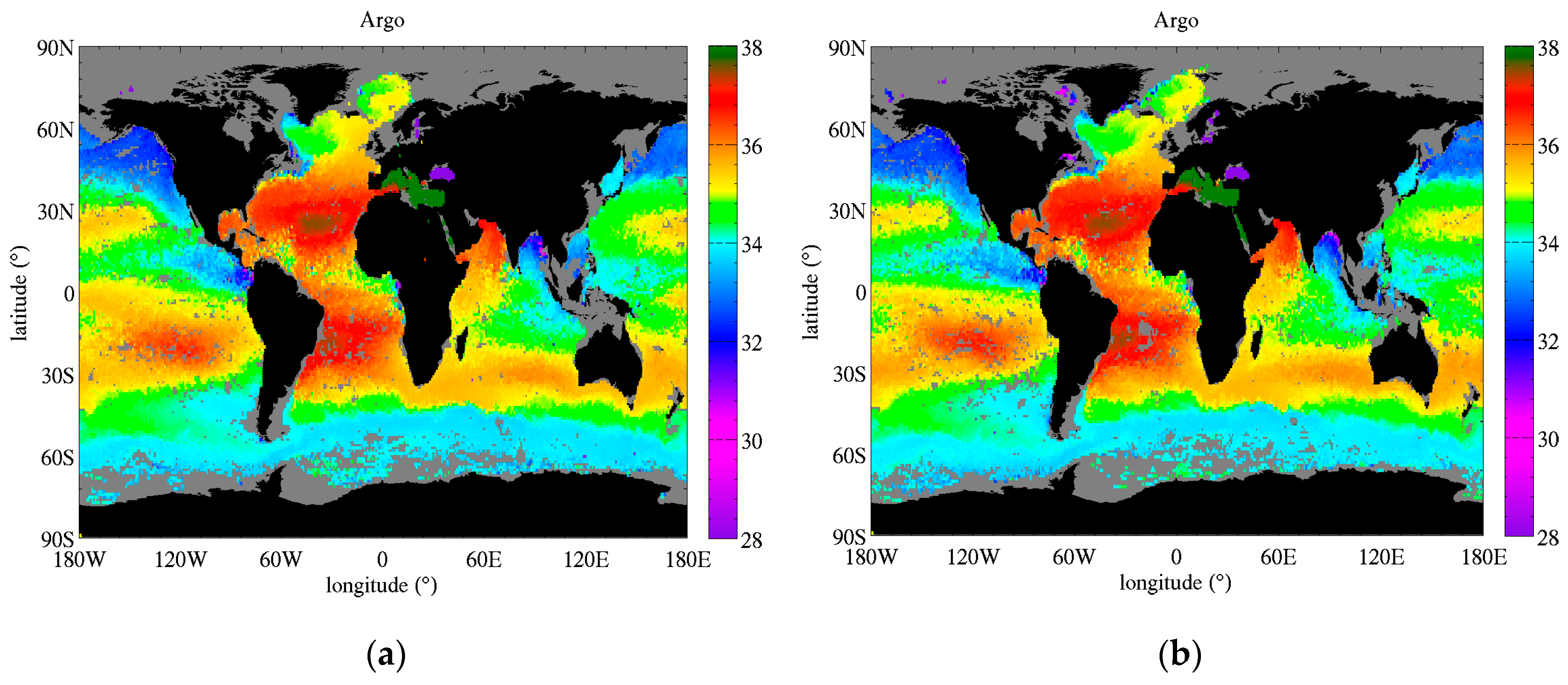
Figure 2 over a map of Argo SSS (top) long term average and (bottom) standard deviation over the period 01/2011–06/2018. They cover various SSS and SST average value, as well as various temporal variability (Table 6). The five oceanic gyres in the Atlantic (#1, 2), Pacific (#5, 6) and South Indian (#8) oceans have SSS which is relatively high (35.3–37.5 psu) and stable (STD 0.07–0.11 psu). Highly variable regions, such as the equatorial Pacific upwelling region (#4), the Amazon plume (#3) and the Tropical Indian Ocean (#10) show seasonal variations of about 0.5–1.0 psu driven by changing fresh water influx from river outflow and large precipitations, and advection by coastal currents and the South Equatorial Current in the Indian Ocean. Low SSS (32.7–33.9 psu) are persistently observed in cold waters at high latitudes (#7, 11, 12), and occur seasonally in big river mouths and plumes (#3). The time series of Argo, SMOS, Aquarius and SMAP SSS in the ROI are reported in Figure 12 and Figure 13. The SMAP and Aquarius SSS are those distributed at the PO.DAAC (Section 2.1).The temporal average and standard deviation of the difference between satellite and Argo SSS are reported for each region in Table 7 and Table 8, respectively. Because SMAP V3 was recently released, we also report results for V2 to emphasize the changes in the latest version of the product. This is discussed at the end of the section. The first paragraph focusses on the latest SMAP, Aquarius and SMOS products.
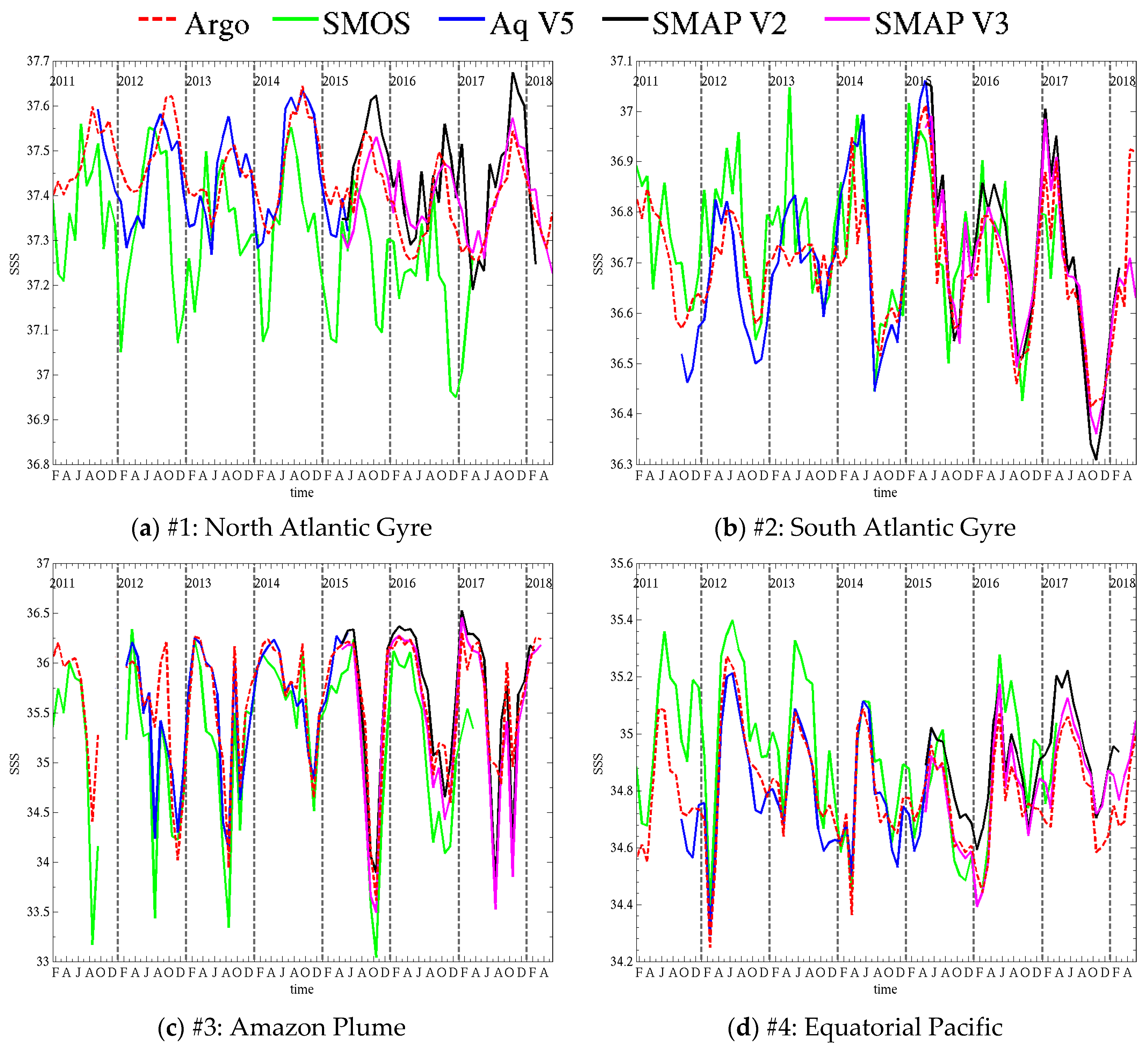
In both Atlantic gyres (#1, #2, Figure 12a,b), SSS seasonal variations are of the order of 0.2–0.3 psu. SMAP V3 and Aquarius show the best performances with overall good agreement in timing and amplitude of the cycles. In the North Atlantic gyre (#1, Figure 12a) SMOS peaks too early in the year compared to Argo and is biased fresh, with too strong freshening events in winter. In the South Atlantic gyre (#2, Figure 12b), SMOS timing is better but the signal is noisier. It does not exhibit excessive freshening like in the North, but there are a few salty peaks (e.g., April 2013) that are not consistent with Argo. The noise is likely due, in part, to our averaging only grid cells where Argo samples exist. Averaging SMOS SSS over the whole ROI would likely smooth out the curves. All the satellites products manage to capture sharp variations, such as the 0.5 psu drop in May–Aug 2014 and 0.4 psu increase in Dec 2014–Apr 2015. Smaller features, such as the peak in Oct 2014, are also reproduced by both SMOS and Aquarius. The Pacific gyres (#5, #6, 
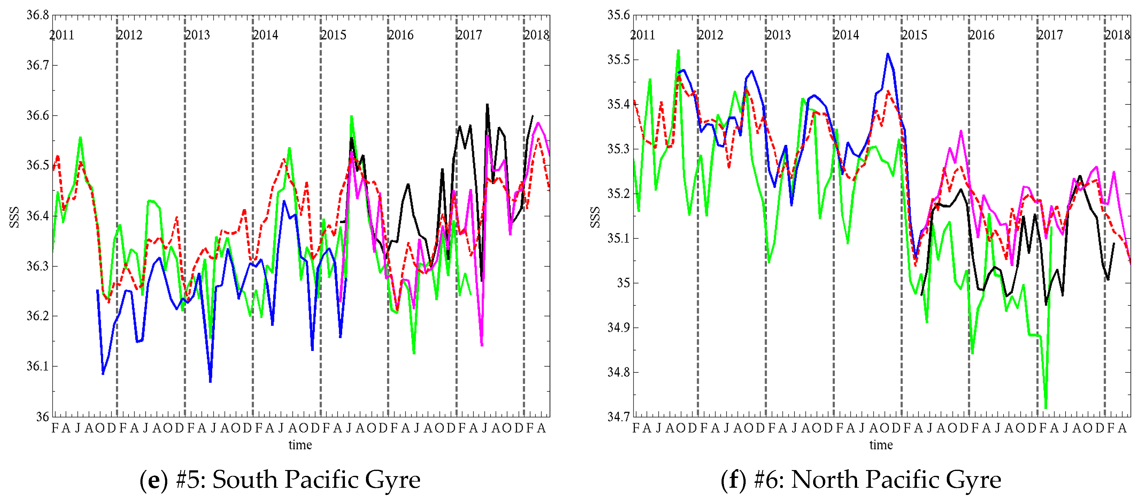
Figure 12e,f) have smaller seasonal variations, of the order of 0.1 psu, but show larger interannual variations. In the Southern Pacific gyre (#5, Figure 12e), SSS drops twice by 0.25 psu, once in the second half of 2011 and once in 2015. After both drops, SSS follows an increasing trend over a few years. Both the drops and trends are well captured by the satellite products. SMOS in particular shows good agreement with Argo in 2011 and limited bias over the whole time series. Aquarius is biased fresh by almost 0.1 psu. SMAP V3 has a good match in phase and amplitude, albeit with a little noise in the signal. In the Northern Pacific gyre (#6, 
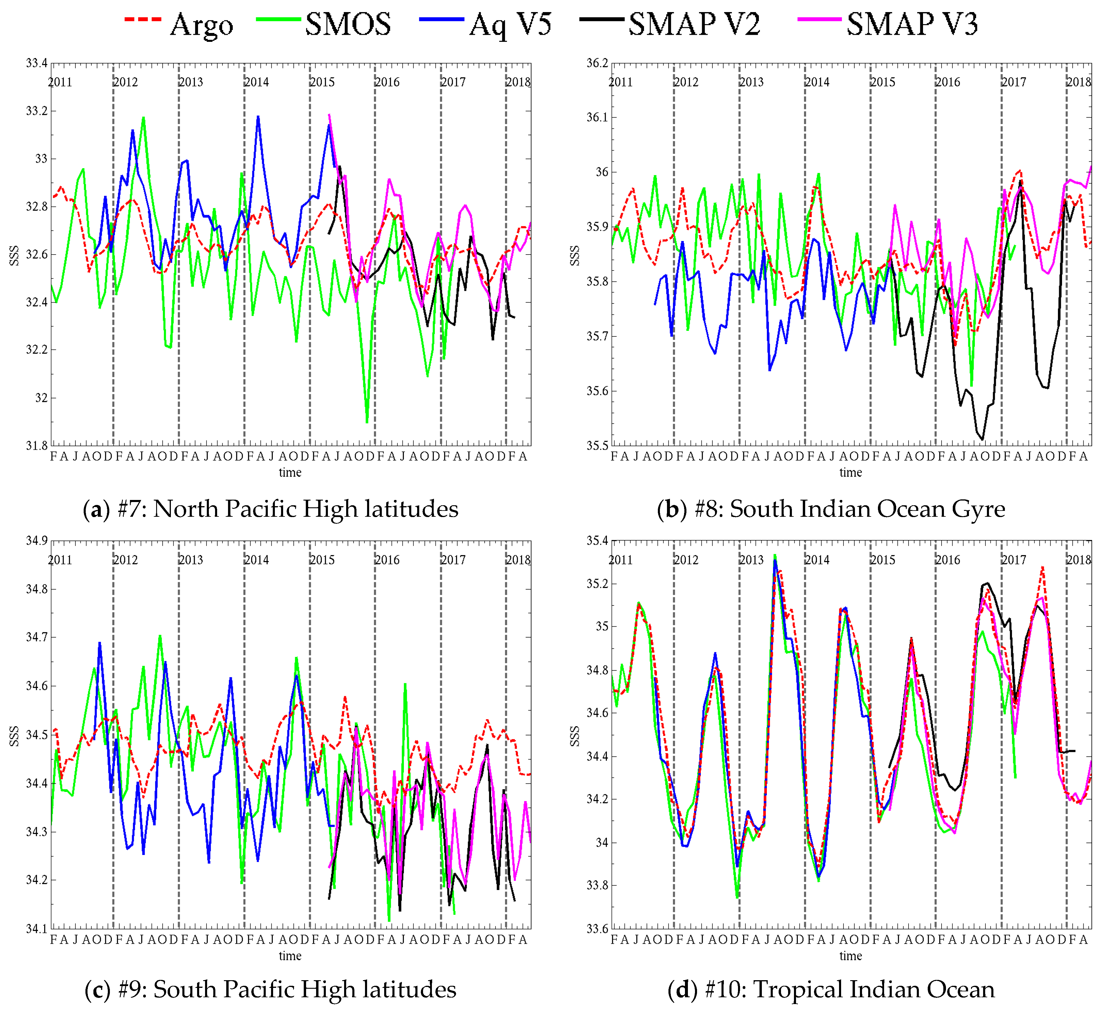
Figure 12f), the seasonal cycles are also small (~0.1 psu) and the largest signal is a 0.35 psu drop in between November 2014 and April 2015. SMOS and Aquarius reproduce accurately the timing of the drop, but the amplitude differs slightly. Both satellites show larger seasonal cycles than Argo, and SMOS is biased fresh (0.1 psu) and tends to peak ahead of Argo during the period 2011–2013. SMAP V3 has the best match to Argo with very small bias (0.02 psu) and good agreement in the seasonal cycles. In the South Indian gyre (#8, Figure 13b), Argo shows similar seasonal cycles almost every year (excluding 2015 and 2016) with peaks early in the year, and peak to peak variations ~0.12 psu. SMOS exhibits a small bias (0.01 psu) but large discrepancies in seasonal variations, except in 2014 and during the 0.2 psu increase from 2016 to 2017. Aquarius has much better seasonal variations, peaking early in the year when Argo does, but is freshly biased by 0.09 psu. SMAP V3 shows the best overall agreement with a small bias and good seasonal variations, although it shows amplified peaks in 2015 and 2016. In the highly variable regions that are the Amazon Plume (#3, Figure 12c), the Equatorial Pacific (#4, Figure 12d) and the Tropical Indian Ocean (#10, Figure 13d), where seasonal variations commonly reach and exceed 0.5 psu, satellite products agree well with Argo overall. In the Amazon Plume (#3, Figure 12c), which shows the largest variations up to 2.5 psu, the timing between satellite and in situ is good with a few exceptions. SMOS tends to be fresh compared to Argo, it has lower SSS peaks and much larger freshening events (up to 1 psu fresher) in the periods July-October. SMAP agrees well with Argo except for the 2017 freshening where it shows a much larger freshening. Overall, Aquarius bias is the smallest and it appears to track seasonal changes the best (e.g., peaks in May and Sept 2013). In a region where SSS is so variable in space and time, it is likely that mismatches between satellite and in situ observation times, locations and scales are causing some of the discrepancies being observed. In the Equatorial Pacific (#4, Figure 12d), seasonal changes are about 0.5 psu, with a larger change of 1 psu in early 2012. All the variations are well captured by SMAP and Aquarius. SMOS tends to overestimate the peak SSS, but the cycles timing is good. The Tropical Indian Ocean (#10, Figure 13d) has a seasonal variation of 0.5 psu–1 psu. All satellites show a very good match to Argo both in timing and amplitude. However, SMOS performances appear to decline starting in 2015 when it starts to underestimate the peaks by 0.1–0.2 psu. All high latitudes ROI (#7, #9, #11, #12, Figure 13a,c,e,f) show decreased performances of the satellite products, with increased bias or standard deviation of the differences with Argo. In the North Pacific high latitudes (#7, Figure 13a), SMAP and Aquarius reproduce well the timing of the seasonal cycles, but the peaks are too high by a few tenths of a psu. SMOS hardly shows seasonal cycles, except maybe in 2011, 2012 and 2016, with large errors in timing or amplitude. In the high latitudes of the South Pacific (#9, Figure 13c) and South Atlantic (#11, Figure 13e), both timing and amplitude of the satellite cycles show significant discrepancies with Argo and SSS is biased by −0.1–+0.2 psu depending on the product. In the high latitudes of the Indian Ocean (#12, Figure 13f), the agreement in the timing and amplitude of the seasonal cycles of all satellites is much better than in the other Southern high latitudes, especially for SMAP V3, but some biases and too salty peaks still occur.
The latest version of the SMAP RSS product (V3) shows improvements over V2 on multiple aspects. Both versions generally have a good agreement with Argo regarding the phase of seasonal variations, including small seasonal cycles in the gyres (#1, #6, Figure 12a,f) and the larger variations in the meanders of the Amazon plume (#3, Figure 12c). However, V2 tends to overestimate the amplitude of these variations at several locations (Gyres #1, #2 and equatorial Pacific #4, Figure 12a,d,f), with peaks too salty by ~0.1 psu. V3 shows substantial improvement in the agreement of the peaks with Argo. In the North Pacific Gyre (#6, Figure 12f), V2 is freshly biased (0.08 psu) and exhibits too large drops in SSS during the first half of the year. V3 improves the bias by 0.06 psu (now slightly too salty) and substantially improves the dynamic range of the seasonal variation by mitigating the drops. In the Amazon Plume (#3, Figure 12c), both versions are generally in agreement, but V2 over-estimates the high salinities in the first half of the year, where V3 matches Argo better. However, the drops in V3 in July and October 2017 are still too large with SSS too low by more than 1 psu compared to Argo. As discussed previously, it is likely that differences in space and time sampling between satellite and in situ observations contribute to the differences in this highly variable region. The Tropical Indian Ocean (#10, Figure 13d) is another variable region and V3 improves on the seasonal variations with SSS decreasing faster and lower after reaching peak value compared to V2 which has peaks that are too wide and underestimates the freshening early in the year by ~0.15 psu. There are a few locations where the seasonal cycles differ between satellite and in situ. In the South Pacific gyre (#5, Figure 12e), V2 exhibits large peaks (Apr 2016, March 2017) not present in Argo. V3 improves SMAP SSS here, but there are still some large variations (e.g., 0.25 psu drop in May 2017) not agreeing with Argo. In the North Pacific high latitude region (#7, Figure 13a), V2 seasonal cycles peak too late compared to V3 and Argo. V3 cycles are in better phase but peaks are too salty. The South Indian gyre (#8, Figure 13b) also shows very substantial improvements in the seasonal cycles of V3 compared to V2 that shows largely overestimated drops in SSS during the southern hemisphere spring, and too fresh peaks early in the year. Finally, all the southern high latitude locations exhibit a significant discrepancy between SMAP SSS (both versions) and Argo, with satellite SSS more variable than in situ. V3 improves on V2 in the high latitudes of the Atlantic (#11, Figure 13e) and Indian (#12, Figure 13f) oceans in terms of bias and slightly in terms of variations. Over all the ROI, V3 reduces the average difference between SMAP SSS and Argo by 0.02–0.11 psu compared to V2 (Table 7), with the mean reduction being 0.07 psu. Its impact on the standard deviation of the difference between SMAP and Argo is relatively small, a reduction of ~0.01 psu on average with larger reductions of 0.023 and 0.033 psu in the North Pacific High latitudes (#7) and Tropical Indian Ocean (#10). This small value is to be compared to the small natural variation of SSS itself, which shows standard deviations of less than 0.2 psu at most locations. In addition, SMAP V3 either improves peaks and troughs, that involve few data points, or corrects biases, limiting its impact on a metric like the standard deviation.

3.3.3. SST-Dependent Bias

A recurring feature of various revisions of SSS products has been the dependence of the SSS biases on SST. This signature is not obvious in the products reported in Figure 9 because of semi-empirical corrections that have been applied to mitigate it in recent years. We report here a summary of various versions of Aquarius and SMAP product that illustrate the issue before examining possible causes in the next section. The SMAP and Aquarius SSS are those distributed at the PO.DAAC (Section 2.1).
The last version of the Aquarius product to not include an empirical correction for the SST-dependent bias was version 3. A map of the SSS difference with Argo for this product (Aquarius SSS-Argo SSS) is reported in Figure 14 (top left, a) and the SSS bias as a function of SST for V3 through V5 is reported in Figure 14 (bottom left, c). SSS errors in Aquarius V3 clearly exhibit a very strong dependence on SST, with SSS too fresh by up to 0.2 psu in warm (>22 °C) waters and too salty by ~0.25 psu in waters between 5 °C and 15 °C. Because of the strong latitudinal dependence of SST, the SSS difference map shows a dipole pattern with too fresh waters at low latitudes and too salty waters at high latitudes, with the separation around 20°N and 30°S. Subsequent versions 4 and 5 have included algorithm enhancements designed to empirically mitigate the SST-dependent bias. The latest version 5 includes a dependence on SST in the surface roughness correction and a modified atmospheric model that substantially decrease the SST-dependent bias. Similar plots for SMAP V2 and V3 products are reported in Figure 14 (top right (b) and bottom right (d)). SMAP V2 also showed substantial SST-dependent bias. However, the dipole pattern is inverted compared to Aquarius, with lower latitude biased salty and higher latitudes biased fresh. The latest version of the SMAP product (V3) is based on the Aquarius V5 algorithm with specific adjustments for SMAP that significantly mitigate the SST-dependent bias compared to V2.
A comparison of the latest SMOS, Aquarius and SMAP products is reported in Figure 15. The left (a) panel reports the SSS bias between satellite and in situ computed as the median of the SSS difference over SST bins 1 °C wide. The right (b) panel reports the variable error computed as the 68% quantile (Q68) of the absolute value of the SSS difference (which matches the standard deviation in case of a normal distribution). Biases in satellite products (Figure 15a) compared to Argo are small over a large range of temperatures. SMOS shows the best overall performance between 4 °C and 24 °C, with a small bias (<0.1 psu) fairly constant in SST. However, the bias dramatically increases for very cold waters (below 4 °C) to exceed +0.8 psu at −1 °C. This bias is much larger than with any other products at any temperature, even including products with strong SST-dependent biases reported in Section 3.3.3. SMOS bias also increases to −0.2 psu in warm waters (30 °C). The increase is not unusual among satellite products which tend to be fresher than in situ observations, and this could reflect in part a difference between shallow (~2 cm) satellite measurement and deeper (5–10 m) Argo measurements. But the amplitude of this bias is larger by 0.1–0.15 psu compared to SMAP and Aquarius and may include additional sources of errors. The latest SMAP and Aquarius products also have small biases over a large range of SST and match the Argo data much better for waters warmer than 24 °C and colder than 4 °C. This is in part due to the empirical adjustments to mitigate the SST-dependent biases. However, not all biases are removed and investigation of the sources of the bias should prove useful in improving the algorithm corrections.
The variable error (Figure 15b) is very similar between the various retrievals. The Q68 is ~0.2 psu for temperatures warmer than 15 °C. There is an increasing trend in the error with decreasing temperature between 22 °C (0.15–0.18 psu) and −2 °C (0.4–0.7 psu). An increase in retrieval random error with decreasing SST is expected because of the reduced radiometric sensitivity to SSS in cold waters. This is illustrated by the inverse of the radiometric sensitivity to SSS reported as a function of SST in Figure 15b (dashed magenta curve labelled dS/dTB, scaled to match the other curves at 18 °C). The decrease in radiometric sensitivity makes the retrievals more sensitive to all source of errors, be it radiometric noise or uncertainty on ancillary parameters, such as SST. In addition, the increase in sensitivity to SST in cold waters amplifies the error due to SST uncertainties. SMAP and Aquarius show the best performances in waters colder than 15 °C, with SMOS error being 0.22 psu larger around 2 °C. Above 10 °C, all satellite products show performance closer to each other, with SMAP having errors smaller by less than 0.03 psu compared to Aquarius, and SMOS being at most 0.07 psu higher. All products also show a small upward trend in warm waters that could be partially due to the impact of precipitation-driven stratification [22,50]. The radiometric sensitivity to SST also increases again in warm waters and there could be an associated impact of uncertainty in SST. The large reduction of samples at the cold end of the temperature range could also contribute to the increase in variable error.
While the empirical algorithm adjustments manage to largely remove the SST-dependent biases, they tend to lack a physical explanation and do not completely resolve the issue. For that reason, we investigate possible causes for the SST-dependent bias in the next section. A better understanding should provide clues for improving further the algorithm.

3.3.4. Impact of the Dielectric Constant Model and Ancillary Temperature on SSS Differences

In the previous section, we showed that differences between the satellite SSS products and in situ SSS exhibit strong regional and seasonal signals that correlate significantly with SST. In this section we quantify the potential impact of some of the models and ancillary data used in the SSS retrieval algorithm. We assess the impact of the differences in the dielectric constant model, ancillary SST products and of the atmospheric model, recently modified for Aquarius, by reprocessing the Aquarius data using alternative parameterizations. We start the reprocessing from the Aquarius top of atmosphere TB from Version 3 because it is the last version to not include an empirical correction for the SST-dependent bias. We successively introduce changes to V3 of the retrieval algorithm, one at a time, to identify their impact. We first change the dielectric constant model to the one by Klein and Swift [39], then change to the ancillary OSTIA SST (both used in the SMOS processing). Finally, we change the atmospheric attenuation model to the one used in V5 which is a return to the original model by Liebe et al. [45].
Each time a change to the retrieval algorithm is applied, the TB is recalibrated as discussed in Section 2.4. In the following, we report the impacts of algorithm changes on the SST-dependent bias (Figure 16). SMOS differences with Argo are computed for distances to the coast of 1000 km or more to mitigate the impact of land contamination on the SSS differences. This does not change substantially our results and essentially shifts the SMOS curves in Figure 16 upwards by 0.03 psu (warm waters) to 0.15 psu (cold waters) compared to the results including also coastal data.
Changing the dielectric constant model for the Aquarius SSS retrievals has a very large impact (changes from solid blue to dashed blue curve in Figure 16). Using the KS model reduces biases for SST between 5 °C and 22 °C compared to the MW model (used in Aquarius V3) and significantly reduces the dependence on SST. There is little change above 22 °C as both models agree and result in fresher SSS compared to Argo measurements. One striking feature of the new curve is the very large increase in bias below 5 °C. In the very cold waters, below 0 °C, the bias now exceeds 1.4 psu. Overall, the KS model brings the Aquarius SST-dependent bias in much better agreement with SMOS bias. But now the Aquarius bias in cold waters is too large, even compared to the already significant SMOS bias of 0.8 psu. Next, we introduce the OSTIA SST in the Aquarius retrieval (blue dotted curve in Figure 16). As illustrated by the example reported in Section 3.2, the impact of the OSTIA SST on the SST-dependent bias is relatively small because of the averaging over large regions and long periods (4 years of data in Figure 16). The impact of differences in ancillary SST can be large locally (>1 psu), but spatial and temporal averaging over large scales, such as latitudinal bands and several seasons, will mitigate the differences. The impact on the average SSS difference is small (±0.01 psu) above 10 °C; it increases slightly in very cold water to result in a bias reduced by ~0.05 psu at 5 °C and ~0.1 psu at 0 °C. The small reduction in bias brings Aquarius results slightly closer to SMOS. An assessment of several SST products for the Aquarius processing identified the CMC product as the one producing the smaller SSS errors compared to in situ data; this product was adopted for the Aquarius final release and the latest SMAP products [46]. Finally, we change to the Liebe atmospheric model in the Aquarius retrieval (blue curve with circles). The new atmospheric model decreases the retrieved SSS by 0.45 psu on average at the cold end (0 °C) and increases it by 0.07 psu at the warm end (30 °C). The bias is very significantly reduced in cold waters. Introducing these three changes (KS model for dielectric constant, OSTIA SST, and Liebe model for atmospheric attenuation) brings the Aquarius retrieval very close to SMOS at almost every temperature. This illustrates the importance of the ancillary data on the performance of the algorithm and suggests that models used in the algorithm (e.g., for the dielectric constant and atmosphere) contribute to the SST-dependent bias. But both sensors still produce too salty retrievals compared to Argo measurements in cold waters, which is likely due to inaccuracies in the KS dielectric constant model. Comparatively, the MW model performs much better in cold waters, but results in more variability of the SSS bias with SST for waters warmer than 5 °C. A new model for the dielectric constant based on extensive laboratory measurements at 1.4 GHz is being developed at George Washington University [54] and may help resolve this issue.

4. Discussion

The latest versions of the SMOS, Aquarius and SMAP SSS products show improved performances with only small biases remaining in open oceans and good accuracy on seasonal and interannual variability. The improvements come in part from empirical adjustments in the retrieval algorithms. The SST-dependent bias correction used by Aquarius and SMAP significantly improves SSS products, but issues remain in cold waters. High southern latitudes still suffer from significant biases, and seasonal variability is still not accurately captured by the satellites. SMOS SSS also exhibit large biases and increased noise in cold waters. While other factors may contribute to the performance issues in cold water, such as sea ice whose presence and quantity can be uncertain [47] and rougher sea surfaces, we find that the model for the dielectric constant of sea water is still questionable and has a significant impact on the retrievals. The KS model used by SMOS results in smaller biases at many temperatures but lead to very large and temperature dependent biases in cold waters. Our results with the KS model are consistent with assessments of microwave radiometers at higher frequencies which found that corrections to TB at the cold end (0 °C) needed to be larger than at the warm end (30 °C) by 0.5 K and 3.7 K at 6 GHz [55] and 37 GHz [56] respectively. It is therefore critical to improve the current dielectric constant models. Recent laboratory measurements performed at L-band at the George Washington University (GWU) [57] have led to a new model that shows promising results with the Aquarius data [54]. These measurements are currently being enhanced by adding more samples at more SST and SSS. When the analytical model using GWU measurements is updated to include the latest measurements, we plan to assess its performances with Aquarius and SMAP data. For SMOS, a product called CEC-LOCEAN DEBIAS v3 includes SST-dependent corrections to the KS model derived from assessments reported here. The capability of the updated GWU model to replace the empirical correction for SMOS should also be tested.

5. Conclusions

We compare satellite SSS products from SMOS, Aquarius and SMAP with in situ measurements from the Argo network of drifting profiling floats. The latest versions of the products show a significant reduction in bias and variable errors in satellite SSS and convergence in the performances of the three sensors. The satellites mostly reproduce the same large-scale patterns as Argo and have small biases in the open ocean overall. Coastal regions benefit from improved corrections compared to previous versions but exhibit larger errors than open oceans. Salty bias at some coastal locations is likely the result of over correction of land contamination. Improving land correction is the focus of current research for future versions of SSS products. The dynamic range of satellite SSS is similar to Argo, with most values between 33.85 psu and 35.85 psu. SMOS shows more prevalent SSS in the range 33.2–33.6 psu than the other products, and all sensors fail to reproduce some of the Argo SSS histogram features due to various regional biases. Time series at various locations around the globe show the good performance of the satellites in reproducing seasonal and interannual changes reported by the in situ data, but disagreements in phase and amplitude of the signals are not uncommon, especially in the high latitudes. Algorithm improvements are still needed for these locations and an example of possible gains is illustrated with SMAP. We have assessed the recently released version 3 of the SMAP product and show that it reduces significantly previous large-scale biases that were correlated with SST and that it improves substantially the seasonal and inter-annual variability, which are now in better agreement with in situ observations. Among the main discrepancies remaining between SSS products is the SST-dependent bias. It varies significantly between products, and results in latitudinal patterns in the satellite SSS error maps when compared to in situ observations. The SST-dependent bias is mitigated through empirical corrections in the retrieval algorithms, but the actual causes for it are not clearly established. We have assessed three possible causes: The sea water dielectric constant model, the ancillary product for SST and the atmospheric model. We find that the impact of the ancillary SST product can be large at small space and time scales. In the cold water of the high latitudes the large SST discrepancies between product are amplified by a lower sensitivity of TB to SSS which results in differences of 1 psu or more in retrieved SSS. However, the impact of the SST ancillary product is relatively small when errors are averaged at large scales or over time. As such, its impact is small on the SST-dependent bias and is mostly noticeable in very cold water (~0.1 psu at 0 °C). We find that the SST-dependent bias is mostly impacted by the dielectric constant model and the atmospheric attenuation model. When substituting the models used for SMOS into the processing of Aquarius observations, we find a much-improved match in the dependence of SSS bias to SST between both sensors. Using the KS dielectric constant model instead of the MW model reduces the mean SSS error by up to 0.2 psu and reduces its variability in the range 5–22 °C. In waters warmer than 20 °C, both dielectric constant models perform similarly to each other. In waters colder than 5 °C, the KS model exhibits very problematic performances. Considering the large errors it produces (>1 psu), and the fast change in the bias with SST (1 psu over a 5 °C range), it appears that the accuracy of the KS model is questionable below 5 °C. This result is consistent with the assessment of microwave radiometers at higher frequencies which found an increase in the KS model bias in cold waters [55,56]. It is doubtful that all the SST-dependent error can be attributed to the dielectric constant model, as other factors can commingle their error and its dependence on SST (e.g., roughness model). In fact, we find that the impact of the atmospheric attenuation and emission model in the latest Aquarius product has a strong correlation with SST. The impact of the new model is larger in cold waters and improves significantly the match with SMOS and generally reduces Aquarius biases. Future research on sea water dielectric constant and atmospheric attenuation at low microwave frequencies will be essential in order to move away from empirical adjustments that are currently necessary to ensure good and consistent performance across all ocean temperatures.

Author Contributions

Conceptualization, E.P.D.; Data curation, E.P.D., J.B. and T.M.; Formal analysis, E.P.D., D.M.L.V., J.B., T.M. and G.L.; Funding acquisition, E.P.D. and D.M.L.V.; Investigation, E.P.D., D.M.L.V., J.B. and T.M.; Methodology, E.P.D.; Software, E.P.D.; Supervision, D.M.L.V. and G.L.; Validation, E.P.D.; Visualization, E.P.D.; Writing—original draft, E.P.D.; Writing—review & editing, E.P.D., D.M.L.V., J.B., T.M. and G.L.

Funding

This research was funded by the National Aeronautics and Space Administration, grant numbers NNX14AR31G and 80NSSC18K1443, and by the CNES/CATDS (Centre Aval de Traitement des Données SMOS) and ESA Climate Change Initiative projects.

Acknowledgments

We would like to thank the Aquarius Cal/Val and Science teams for the useful discussions concerning this study.

Conflicts of Interest

The authors declare no conflict of interest. The funders had no role in the design of the study; in the collection, analyses, or interpretation of data; in the writing of the manuscript, or in the decision to publish the results.

References

  1. Font, J.; Camps, A.; Borges, A.; Martin-Neira, M.; Boutin, J.; Reul, N.; Kerr, Y.H.; Hahne, A.; Mecklenburg, S. SMOS: The challenging sea surface salinity measurement from space. Proc. IEEE 2010, 98, 649–665. [Google Scholar] [CrossRef]
  2. Kerr, Y.H.; Waldteufel, P.; Wigneron, J.-P.; Delwart, S.; Cabot, F.; Boutin, J.; Escorihuela, M.-J.; Font, J.; Reul, N.; Gruhier, C.; et al. The SMOS Mission: New Tool for Monitoring Key Elements of the Global Water Cycle. Proc. IEEE 2010, 98, 666–687. [Google Scholar] [CrossRef]
  3. Lagerloef, G.; Colomb, F.R.; Le Vine, D.; Wentz, F.; Yueh, S.; Ruf, C.; Lilly, J.; Gunn, J.; Chao, Y.; deCharon, A.; et al. The Aquarius/SAC-D Mission: Designed to Meet the Salinity Remote-Sensing Challenge. Oceanography 2008, 21, 68–81. [Google Scholar] [CrossRef] [Green Version]
  4. Le Vine, D.M.; Lagerloef, G.S.E.; Torrusio, S.E. Aquarius and remote sensing of sea surface salinity from space. Proc. IEEE 2010, 98, 688–703. [Google Scholar] [CrossRef]
  5. Le Vine, D.M.; Dinnat, E.P.; Meissner, T.; Yueh, S.H.; Wentz, F.J.; Torrusio, S.E.; Lagerloef, G. Status of Aquarius/SAC-D and Aquarius Salinity Retrievals. IEEE J. Sel. Top. Appl. Earth Obs. Remote Sens. 2015, 8, 5401–5415. [Google Scholar] [CrossRef]
  6. Grodsky, S.A.; Reul, N.; Lagerloef, G.; Reverdin, G.; Carton, J.A.; Chapron, B.; Quilfen, Y.; Kudryavtsev, V.N.; Kao, H.Y. Haline hurricane wake in the Amazon/Orinoco plume: AQUARIUS/SACD and SMOS observations. Geophys. Res. Lett. 2012, 39, 4–11. [Google Scholar] [CrossRef]
  7. Grodsky, S.A.; Reverdin, G.; Carton, J.A.; Coles, V.J. Year-to-year salinity changes in the Amazon plume: Contrasting 2011 and 2012 Aquarius/SACD and SMOS satellite data. Remote Sens. Environ. 2014, 140, 14–22. [Google Scholar] [CrossRef]
  8. Gierach, M.M.; Vazquez-Cuervo, J.; Lee, T.; Tsontos, V.M. Aquarius and SMOS detect effects of an extreme Mississippi River flooding event in the Gulf of Mexico. Geophys. Res. Lett. 2013, 40, 5188–5193. [Google Scholar] [CrossRef] [Green Version]
  9. Hernandez, O.; Boutin, J.; Kolodziejczyk, N.; Reverdin, G.; Martin, N.; Gaillard, F.; Reul, N.; Vergely, J.L. SMOS salinity in the subtropical North Atlantic salinity maximum: 1. Comparison with Aquarius and in situ salinity. J. Geophys. Res. C Ocean. 2014, 119, 8878–8896. [Google Scholar] [CrossRef] [Green Version]
  10. Garcia-Eidell, C.; Comiso, J.C.; Dinnat, E.; Brucker, L. Satellite observed salinity distributions at high latitudes in the Northern Hemisphere: A comparison of four products. J. Geophys. Res. Ocean. 2017, 122, 7717–7736. [Google Scholar] [CrossRef]
  11. Ebuchi, N.; Abe, H. Evaluation of sea surface salinity observed by Aquarius and SMOS. In Proceedings of the International Geoscience and Remote Sensing Symposium (IGARSS), Melbourne, Australia, 21–26 July 2013; pp. 656–659. [Google Scholar]
  12. Dinnat, E.; Boutin, J.; Le Vine, D.; Yin, X. Inter-Comparison of Aquarius and SMOS Calibration and Impact on Sea Surface Salinity Products. In Proceedings of the American Geophysical Union, Fall meeting, San Francisco, CA, USA, 15–19 December 2014. [Google Scholar]
  13. Pablos, M.; Piles, M.; Gonzalez-Gambau, V.; Vall-Llossera, M.; Camps, A.; Martinez, J. SMOS and Aquarius radiometers: Inter-comparison over selected targets. IEEE J. Sel. Top. Appl. Earth Obs. Remote Sens. 2014, 7, 3833–3844. [Google Scholar] [CrossRef]
  14. Yueh, S.H.; West, R.; Wilson, W.J.; Li, F.K.; Njoku, E.G.; Rahmat-Samii, Y. Error sources and feasibility for microwave remote sensing of ocean surface salinity. IEEE Trans. Geosci. Remote Sens. 2001, 39, 1049–1060. [Google Scholar] [CrossRef]
  15. Dinnat, E.P.; Boutin, J.; Caudal, G.; Etcheto, J.; Waldteufel, P. Influence of sea surface emissivity model parameters at L-band for the estimation of salinity. Int. J. Remote Sens. 2002, 23, 5117–5122. [Google Scholar] [CrossRef]
  16. Dinnat, E.P.; Boutin, J.; Caudal, G.; Etcheto, J. Issues concerning the sea emissivity modeling at L band for retrieving surface salinity. Radio Sci. 2003, 38. [Google Scholar] [CrossRef] [Green Version]
  17. Boutin, J.; Waldteufel, P.; Martin, N.; Caudal, G.; Dinnat, E. Surface salinity retrieved from SMOS measurements over the global ocean: Imprecisions due to sea surface roughness and temperature uncertainties. J. Atmos. Ocean. Technol. 2004, 21, 1432–1447. [Google Scholar] [CrossRef]
  18. Waldteufel, P.; Floury, N.; Dinnat, E.P.; Caudal, G. Ionospheric effects for L-band 2-D interferometric radiometry. IEEE Trans. Geosci. Remote Sens. 2004, 42, 105–118. [Google Scholar] [CrossRef]
  19. Meissner, T.; Wentz, F.J.; Le Vine, D.M. Aquarius Salinity Retrieval Algorithm Algorithm Theoretical Basis Document (ATBD) End of Mission Version. RSS Technical Report 120117; Remote Sensing Systems: Santa Rosa, CA, USA, 2017; p. 104. [Google Scholar]
  20. Le Vine, D.M.; Dinnat, E.P.; Meissner, T.; Wentz, F.J.; Kao, H.Y.; Lagerloef, G.; Lee, T. Status of Aquarius and salinity continuity. Remote Sens. 2018, 10, 1585. [Google Scholar] [CrossRef]
  21. Yueh, S.; Tang, W.; Fore, A.; Hayashi, A.; Song, Y.; Lagerloef, G. Aquarius geophysical model function and combined active passive algorithm for ocean surface salinity and wind retrieval. J. Geophys. Res. Ocean. 2014, 119, 5360–5379. [Google Scholar] [CrossRef] [Green Version]
  22. Tang, W.; Yueh, S.; Fore, A.; Neumann, G.; Hayashi, A.; Lagerloef, G. The rain effect on Aquarius’ L-band sea surface brightness temperature and radar backscatter. Remote Sens. Environ. 2013, 137, 147–157. [Google Scholar] [CrossRef]
  23. Chassignet, E.; Hurlburt, H.; Metzger, E.J.; Smedstad, O.; Cummings, J.; Halliwell, G.; Bleck, R.; Baraille, R.; Wallcraft, A.; Lozano, C.; et al. US GODAE: Global ocean prediction with the HYbrid Coordinate Ocean Model (HYCOM). Oceanography 2009, 22, 64–75. [Google Scholar] [CrossRef]
  24. Boutin, J. CATDS Ocean Salinity Level 3 products–Differences & Pros/Cons. Available online: http://www.catds.fr/content/download/68781/file/OS_L3_products_Differences_and_ProsCons.pdf (accessed on 26 March 2019).
  25. Kolodziejczyk, N.; Boutin, J.; Vergely, J.L.; Marchand, S.; Martin, N.; Reverdin, G. Mitigation of systematic errors in SMOS sea surface salinity. Remote Sens. Environ. 2016, 180, 164–177. [Google Scholar] [CrossRef]
  26. Boutin, J.; Vergely, J.L.; Marchand, S.; D’Amico, F.; Hasson, A.; Kolodziejczyk, N.; Reul, N.; Reverdin, G.; Vialard, J. New SMOS Sea Surface Salinity with reduced systematic errors and improved variability. Remote Sens. Environ. 2018, 214, 115–134. [Google Scholar] [CrossRef]
  27. Olmedo, E.; Martínez, J.; Turiel, A.; Ballabrera-Poy, J.; Portabella, M. Debiased non-Bayesian retrieval: A novel approach to SMOS Sea Surface Salinity. Remote Sens. Environ. 2017, 193, 103–126. [Google Scholar] [CrossRef]
  28. Carval, T.; Keeley, R.; Takatsuki, Y.; Yoshida, T.; Loch, S.; Schmid, C.; Goldsmith, R.; Wong, A.; McCreadie, R.; Thresher, A.; et al. Argo User ’s Manual; Ifremer: Brest, France, 2017. [Google Scholar]
  29. Piepmeier, J.; Brown, S.; Gales, J.; Hong, L.; Lagerloef, G.; Le Vine, D.; de Matthaeis, P.; Meissner, T.; Bindlish, R.; Jackson, T.; et al. Aquarius Radiometer Post-Launch Calibration for Product Version 2; National Aeronautics and Space Administration: Washington, DC, USA, 2013.
  30. Dinnat, E.P.; Le Vine, D.M.; Piepmeier, J.R.; Brown, S.T.; Hong, L. Aquarius L-band Radiometers Calibration Using Cold Sky Observations. IEEE J. Sel. Top. Appl. Earth Obs. Remote Sens. 2015, 8, 5433–5449. [Google Scholar] [CrossRef]
  31. Martín-Neira, M.; Oliva, R.; Corbella, I.; Torres, F.; Duffo, N.; Durán, I.; Kainulainen, J.; Closa, J.; Zurita, A.; Cabot, F.; et al. SMOS instrument performance and calibration after six years in orbit. Remote Sens. Environ. 2016, 180, 19–39. [Google Scholar] [CrossRef] [Green Version]
  32. Peng, J.; Misra, S.; Piepmeier, J.R.; Dinnat, E.P.; Hudson, D.; Le Vine, D.M.; De Amici, G.; Mohammed, P.N.; Bindlish, R.; Yueh, S.H.; et al. Soil Moisture Active/Passive L-Band Microwave Radiometer Postlaunch Calibration. IEEE Trans. Geosci. Remote Sens. 2017, 55, 5339–5354. [Google Scholar] [CrossRef]
  33. Zine, S.; Boutin, J.; Font, J.; Reul, N.; Waldteufel, P.; Gabarro, C.; Tenerelli, J.; Petitcolin, F.; Vergely, J.L.; Talone, M.; et al. Overview of the SMOS sea surface salinity prototype processor. IEEE Trans. Geosci. Remote Sens. 2008, 46, 621–644. [Google Scholar] [CrossRef]
  34. Meissner, T.; Wentz, F.J.; Ricciardulli, L. The emission and scattering of L-band microwave radiation from rough ocean surfaces and wind speed measurements from the Aquarius sensor. J. Geophys. Res. C Ocean. 2014, 119, 6499–6522. [Google Scholar] [CrossRef] [Green Version]
  35. Piepmeier, J.R.; Hong, L.; Pellerano, F.A. Aquarius L-Band Microwave Radiometer: 3 Years of Radiometric Performance and Systematic Effects. IEEE J. Sel. Top. Appl. Earth Obs. Remote Sens. 2015, 8, 5416–5423. [Google Scholar] [CrossRef]
  36. Lagerloef, G.; Kao, H.-Y.; Meissner, T.; Vazquez, J. Aquarius Salinity Validation Analysis; Data Version 4.0; National Aeronautics and Space Administration: Washington, DC, USA, 2015.
  37. Yin, X.; Boutin, J.; Spurgeon, P. First assessment of SMOS data over open ocean: Part I-pacific ocean. IEEE Trans. Geosci. Remote Sens. 2012, 50, 1648–1661. [Google Scholar] [CrossRef]
  38. Meissner, T.; Wentz, F.J.; Le Vine, D.M. The salinity retrieval algorithms for the NASA Aquarius version 5 and SMAP version 3 releases. Remote Sens. 2018, 10, 1121. [Google Scholar] [CrossRef]
  39. Klein, L.A.; Swift, C.T. An improved model for the dielectric constant of sea water at microwave frequencies. IEEE J. Ocean. Eng. 1977, AP-25, 104–111. [Google Scholar] [CrossRef]
  40. Meissner, T.; Wentz, F.J. The complex dielectric constant of pure and sea water from microwave satellite observations. IEEE Trans. Geosci. Remote Sens. 2004, 42, 1836–1849. [Google Scholar] [CrossRef] [Green Version]
  41. Meissner, T.; Wentz, F.J. The Emissivity of the Ocean Surface Between 6 and 90 GHz Over a Large Range of Wind Speeds and Earth Incidence Angles. IEEE Trans. Geosci. Remote Sens. 2012, 50, 3004–3026. [Google Scholar] [CrossRef]
  42. Donlon, C.J.; Martin, M.; Stark, J.; Roberts-Jones, J.; Fiedler, E.; Wimmer, W. The Operational Sea Surface Temperature and Sea Ice Analysis (OSTIA) system. Remote Sens. Environ. 2012, 116, 140–158. [Google Scholar] [CrossRef]
  43. Reynolds, R.W.; Smith, T.M.; Liu, C.; Chelton, D.B.; Casey, K.S.; Schlax, M.G. Daily high-resolution-blended analyses for sea surface temperature. J. Clim. 2007, 20, 5473–5496. [Google Scholar] [CrossRef]
  44. Liebe, H.J.; Rosenkranz, P.W.; Hufford, G.A. Atmospheric 60-GHz oxygen spectrum: New laboratory measurements and line parameters. J. Quant. Spectrosc. Radiat. Transf. 1992, 48, 629–643. [Google Scholar] [CrossRef]
  45. Wentz, F.J.; Meissner, T. Atmospheric absorption model for dry air and water vapor at microwave frequencies below 100GHz derived from spaceborne radiometer observations. Radio Sci. 2016, 51, 381–391. [Google Scholar] [CrossRef]
  46. Meissner, T.; Wentz, F.J.; Scott, J.; Vazquez-Cuervo, J. Sensitivity of Ocean Surface Salinity Measurements From Spaceborne L-Band Radiometers to Ancillary Sea Surface Temperature. IEEE Trans. Geosci. Remote Sens. 2016, 54, 7105–7111. [Google Scholar] [CrossRef]
  47. Dinnat, E.P.; Brucker, L. Improved Sea Ice Fraction Characterization for L-Band Observations by the Aquarius Radiometers. IEEE Trans. Geosci. Remote Sens. 2017, 55, 1285–1304. [Google Scholar] [CrossRef]
  48. Tian-Kunze, X.; Kaleschke, L.; Maaß, N.; Mäkynen, M.; Serra, N.; Drusch, M.; Krumpen, T. SMOS-derived thin sea ice thickness: Algorithm baseline, product specifications and initial verification. Cryosphere 2014, 8, 997–1018. [Google Scholar] [CrossRef]
  49. Maaß, N.; Kaleschke, L.; Tian-Kunze, X.; Drusch, M. Snow thickness retrieval over thick Arctic sea ice using SMOS satellite data. Cryosphere 2013, 7, 1971–1989. [Google Scholar] [CrossRef] [Green Version]
  50. Boutin, J.; Chao, Y.; Asher, W.E.; Delcroix, T.; Drucker, R.; Drushka, K.; Kolodziejczyk, N.; Lee, T.; Reul, N.; Reverdin, G.; et al. Satellite and In Situ Salinity: Understanding Near-surface Stratification and Sub-footprint Variability. Bull. Am. Meteorol. Soc. 2016, 97, 1391–1408. [Google Scholar] [CrossRef]
  51. Hasson, A.; Puy, M.; Boutin, J.; Guilyardi, E.; Morrow, R. Northward Pathway Across the Tropical North Pacific Ocean Revealed by Surface Salinity: How do El Niño Anomalies Reach Hawaii? J. Geophys. Res. Ocean. 2018, 123, 2697–2715. [Google Scholar] [CrossRef]
  52. Chaigneau, A.; Morrow, R. Surface temperature and salinity variations between Tasmania and Antartica, 1993–1999. J. Geophys. Res. 2002, 107, 22–27. [Google Scholar] [CrossRef]
  53. Yin, X.; Boutin, J.; Spurgeon, P. Biases between measured and simulated SMOS brightness temperatures over ocean: Influence of sun. IEEE J. Sel. Top. Appl. Earth Obs. Remote Sens. 2013, 6, 1341–1350. [Google Scholar] [CrossRef]
  54. Zhou, Y.; Lang, R.H.; Dinnat, E.P.; Le Vine, D.M. L-Band Model Function of the Dielectric Constant of Seawater. IEEE Trans. Geosci. Remote Sens. 2017, 55, 6964–6974. [Google Scholar] [CrossRef]
  55. Shibata, A. Description of GCOM-W1 AMSR2 Sea Surface Temperature Algorithm. In Descriptions of GCOM-W1 AMSR2 Level 1R and Level 2 Algorithms; Japan Aerospace Exploration Agency: Tokyo, Japan, 2013; p. 119. [Google Scholar]
  56. Shibata, A. A change of microwave radiation from the ocean surface induced by air-sea temperature difference. Radio Sci. 2003, 38. [Google Scholar] [CrossRef]
  57. Lang, R.; Zhou, Y.; Utku, C.; Le Vine, D. Accurate measurements of the dielectric constant of seawater at L band. Radio Sci. 2016, 51, 2–24. [Google Scholar] [CrossRef] [Green Version]
Figure 1. Timeline of satellite sea surface salinity (SSS) products availability. The Soil Moisture and Ocean Salinity (SMOS) SSS is available starting Jan 2010 (onward). The Aquarius product is available from Aug 25, 2011 until June 7, 2015 when the spacecraft bus failed. The Soil Moisture Active Passive (SMAP) product is available starting April 2015 (onward).
Remotesensing 11 00750 g001
Figure 2. Map of long-term SSS patterns and variability derived from in situ Argo measurements. (a) Map of the average Argo SSS in 1° × 1° grid cells in latitude and longitude over the period Jan 2011–June 2018. (b) Standard deviation over time of monthly 1° × 1° average Argo SSS maps. The numbered red and black boxes report the limits for the regions of interest used to assess temporal variability of SSS (see text).
Remotesensing 11 00750 g002aRemotesensing 11 00750 g002b
Figure 3. Schematic of Aquarius empirical calibration and SSS retrieval algorithm. The first step (top left) is to calibrate the antenna temperatures (TA) measured by the sensor using the forward radiative transfer model that will also be used in the retrieval to compute expected TA (right hand side of the diagram). This step assumes a reference SSS (e.g., from a numerical model) and uses the same ancillary data (e.g., sea surface temperature, wind, atmospheric parameters, …) that are used in the retrieval step. Global averages over seven-day periods for TA are used in the calibration to mitigate the impact of uncertainty in the reference SSS and other errors. The retrieval steps are illustrated on the left side, starting with TA calibrated at the top, going down the chain to remove unwanted contributions and ultimately retrieve TB at the ocean surface corrected for surface roughness. The last step is retrieving the SSS from the roughness-corrected TB. Other SSS product algorithm will differ slightly. More details are given in Section 2.3.
Remotesensing 11 00750 g003
Figure 4. Differences in TB and SSS due to differences between the dielectric constant model by Klein and Swift [39] and Meissner and Wentz [41]. (a) Differences in brightness temperature at L-band for a flat surface and an incidence angle of 38° (similar to Aquarius middle beam). (b) Differences in retrieved SSS when assuming KS the truth (i.e., used to compute TB from assumed SST0 and SSS0) and using MW for retrieving SSS from TB and the same SST0. The shaded area reports unlikely combinations of SSS and SST (i.e., less than 5 Argo records over the last period 2000–2018).
Remotesensing 11 00750 g004
Figure 5. Differences in weekly average SST between OSTIA and National Oceanic and Atmospheric Administration (NOAA) OI V2 products. Difference maps are averaged weekly from daily products at 0.25° resolution in latitude/longitude during the period September 2011–August 2015. The top row (a,b) shows two examples of SST differences maps. The dates are chosen to show examples of (a) smaller (Feb 2012) and (b) larger (July 2012) differences in SST. Grey areas report sea ice fraction (from OSTIA) of 0.15 or above. The temporal evolution of SST differences is reported in panel (c) through several statistical indicators. The curves report the time series of (red) mean and (dashed-black) median difference in global weekly maps and the percentiles of the absolute value of the SST differences between 70% and 99% (see text in Section 3.2). Panel (d) reports the histogram of SST difference for the map reported in (b) (y-axis unit is 1000 grid cells).
Remotesensing 11 00750 g005aRemotesensing 11 00750 g005b
Figure 6. Impact of SST differences on TB and retrieved SSS. (a) Map of SST differences (°C) between OSTIA and NOAA OI interpolated at the Aquarius ground tracks (same week as in (b) in Figure 5, ascending orbits). (b) Differences in TB (K) for a flat surface due to the differences in SST in the left figure. (c) Differences in retrieved SSS (psu) due to differences in TB reported in the middle figure.
Remotesensing 11 00750 g006
Figure 7. Differences in Aquarius TB due to differences between OSTIA and NOAA OI versus time, for the middle beam in vertical polarization. The TB difference is (grey) for each Aquarius 1.44 s footprint and (red) averaged globally over seven days.
Remotesensing 11 00750 g007
Figure 8. Global map of SSS from satellite sensors and in situ measurements averaged over several years. On the left: (a) Argo SSS, (c) SMOS SSS, and (e) Aquarius SSS are averaged over the Aquarius era (i.e., Sept 2011–May 2015). On the right: (b) Argo SSS, (d) SMOS SSS, and (f) SMAP SSS are averaged over the period April 2015–June 2018. Grey color reports missing data.
Remotesensing 11 00750 g008aRemotesensing 11 00750 g008b
Figure 9. Map of SSS difference between satellite retrievals and in situ Argo observations for (a) SMOS, (b) Aquarius V5, and (c) SMAP V3. The maps are computed from long-term averages of monthly SSS maps over the Aquarius era (i.e., Sept 2011–May 2015) for SMOS and Aquarius, and the period April 2015–June 2018 for SMAP. The green dashed line between 60°S and 45°S marks the average location of the Antarctic convergence that parts cold and dense surface Antarctic waters and sub-Antarctic regions North of it.
Remotesensing 11 00750 g009
Figure 10. Maps of meridional gradients of (a) SSS in psu per degree of latitude and (b) SST in °C per degree of latitude computed from monthly Argo maps. The magenta line reports the approximate location of the Antarctic Convergence.
Remotesensing 11 00750 g010
Figure 11. Histogram of SSS from (red) Argo in situ measurements and satellite SSS measurements by (a) SMOS and Aquarius, and (b) SMAP. They are computed from global monthly maps at 1° × 1° resolution in latitude and longitude over the period (a) Sept 2011–May 2015 and (b) April 2015–June 2018. The x-axis sampling is 0.05 psu; the x-axis is cropped between 30 and 40 psu.
Remotesensing 11 00750 g011
Figure 12. Time series of SSS from (red) Argo, (green) SMOS, (blue) Aquarius and (black) SMAP for regions of interest 1–6 reported in Figure 2.
Remotesensing 11 00750 g012aRemotesensing 11 00750 g012b
Figure 13. Time series of SSS from (red) Argo, (green) SMOS, (blue) Aquarius and (black) SMAP for regions of interest 7–12 reported in Figure 2.
Remotesensing 11 00750 g013aRemotesensing 11 00750 g013b
Figure 14. SST dependence of SSS bias for various versions of SMAP and Aquarius products. Top row (a,b) reports maps of SSS difference between satellite and in situ for (a) Aquarius V3 and (b) SMAP V2 averaged over several years from monthly products. The bottom row (c,d) reports the SSS difference between satellite and in situ SSS as a function of SST for (c) Aquarius V3 (red), V4 (green) and V5 (blue) and (d) SMAP V2 (green) and V3 (blue). The vertical bars in the background report the statistical distribution of the samples as a function of SST (amplitude is normalized to the amplitude of SSS curves).
Remotesensing 11 00750 g014
Figure 15. SSS (a) bias and (b) variable difference between satellite retrievals and in situ Argo measurements as a function of SST for SMOS CPDC RE05, and the latest Aquarius (V5) and SMAP (V3) versions. SMOS includes filtering of land contamination by removing data closer than 1000 km from the coast. The vertical bars in the background report the statistical distribution of the samples as a function of SST. The magenta dashed curve in the right (b) panel reports the relative change in the inverse of the radiometric sensitivity to SSS as a function of SST, scaled to match SSS error curves at 18 °C.
Remotesensing 11 00750 g015
Figure 16. Comparison of SST-dependent bias between SMOS and Aquarius and impact of retrieval parameters. The plot reports the difference between satellite and in situ SSS binned as a function of SST and computed from monthly SSS maps over the period Sept 2011–May 2015. Satellite SSS are (Red) SMOS, and (Blue) Aquarius V3. The Aquarius V3 curves are for (plain) the nominal product, (dashed) V3 reprocessed using the KS dielectric constant model, (dotted) using KS model and OSTIA ancillary SST, and (plain and circles) using the KS model, the OSTIA SST and the adjusted atmospheric model from Aquarius V5.
Remotesensing 11 00750 g016
Table 1. Reduction in the amount of Aquarius L2 samples over ocean due to filtering based on quality control flags.
QC FlagData Reduction
(1) Non science mode, event, anomalous TA, TOI TB or surface TB1.92%
(2) Land contamination13.50%
(3) Sea ice contamination24.62%
(4) SSS less than 024.51%
(5) Regions of severe radio frequency interference (RFI)2.67%
(6) Large RFI correction applied2.72%
(7) Celestial Sky Contamination5.94%
(8) All flags39.69%
Table 2. Recalibration offset for Aquarius brightness temperatures in Kelvin applied when changing the dielectric constant model to Klein and Swift (KS) and/or the ancillary SST product to Operational Sea Surface Temperature and Sea Ice Analysis (OSTIA) in the retrieval algorithm.
KSOSTIA SSTKS and OSTIA
V-polH-polV-polH-polV-polH-pol
Beam 1−0.113−0.095−0.009−0.007−0.121−0.102
Beam 2−0.120−0.089−0.010−0.007−0.128−0.094
Beam 3−0.130−0.083−0.010−0.006−0.138−0.088
Table 3. SSS distribution statistics for satellite products and in situ observation from the Argo network (all values in psu). The SMOS, Aquarius and the top Argo row are computed for the Aquarius era (Sept 2011–May 2015), the second Argo row and SMAP results are computed during the SMAP era (04/2015–06/2018).
Median2.50%16%84%97.50%
Argo34.9032.7533.9235.7436.85
SMOS CPDC (filtered land)34.8233.2333.9935.7636.90
Aquarius V534.8532.7133.9735.6936.85
Argo (SMAP period)34.8332.6533.9035.8437.00
SMAP V334.7832.6133.8535.8537.00
SMAP V234.7832.4133.7835.8637.23
Table 4. Start and end date for the statistics of the differences between satellite products and Argo in situ data.
SMOS CPDCAquarius V3Aquarius V5SMAP V2SMAP V3
Start DateJan-2011Sep-2011Sep-2011Apr-2015Apr-2015
End DateMar-2017Apr-2015May-2015Feb-2018Jun-2018
Table 5. Longitude and latitude (in °) limits for the regions of interest in Figure 2.
Region nameLong. WestLong. EastLat. NorthLat. South
North Atlantic Gyre−42.5−282428
South Atlantic Gyre−16.8−10.5−24.7−17.3
Amazon Plume−46.5−43411
Equatorial Pacific−132.8−93.4−2.62.6
South Pacific Gyre−146.3−108.6−23.4−16.6
North Pacific Gyre−165.1−134.823.731.8
North Pacific High latitudes−180.2−144.14650
South Indian Ocean Gyre75.299.2−33.1−26.7
South Pacific High latitudes−172−140−51.5−46.8
Tropical Indian Ocean6884−11.5−4.5
South Atlantic High latitudes−208−50−45
Table 6. Argo SSS and SST median and STD in regions of interest.
ROI #Region NameMedian SSS (psu)STD SSS (psu)Median SST (°C)STD SST (°C)
1North Atlantic Gyre37.420.0923.961.77
2South Atlantic Gyre36.700.1323.231.67
3Amazon Plume35.820.6327.870.94
4Equatorial Pacific34.780.1925.071.77
5South Pacific Gyre36.370.0825.901.29
6North Pacific Gyre35.260.1122.531.73
7North Pacific High latitudes32.640.107.412.82
8South Indian Ocean Gyre35.850.0720.891.77
9South Pacific High latitudes34.480.059.971.30
10Tropical Indian Ocean34.610.3928.510.85
11South Atlantic High latitudes33.830.055.391.19
12South Indian Ocean High latitudes33.910.137.191.35
Table 7. Average (median) difference (psu) between satellite SSS and Argo SSS.
ROI#Region NameSMOS CPDCAquarius V5SMAP V2SMAP V3
1North Atlantic Gyre−0.14−0.030.060.01
2South Atlantic Gyre0.04−0.020.050.02
3Amazon Plume−0.31−0.010.13−0.06
4Equatorial Pacific0.10−0.030.120.04
5South Pacific Gyre−0.04−0.080.070.00
6North Pacific Gyre−0.100.02−0.080.02
7North Pacific High latitudes−0.160.11−0.100.02
8South Indian Ocean Gyre0.01−0.09−0.120.03
9South Pacific High latitudes−0.04−0.09−0.14−0.12
10Tropical Indian Ocean−0.07−0.020.11−0.03
11South Atlantic High latitudes0.120.22−0.140.07
12South Indian Ocean High latitudes0.070.22−0.140.03
Table 8. Standard deviation (psu) of the difference between satellite and Argo SSS.
ROI#Region NameSMOS CPDCAquarius V5SMAP V2SMAP V3
1North Atlantic Gyre0.1340.0620.0820.065
2South Atlantic Gyre0.0970.0860.0620.078
3Amazon Plume0.4000.3170.3570.367
4Equatorial Pacific0.1290.0690.0780.075
5South Pacific Gyre0.0740.0690.0950.077
6North Pacific Gyre0.1180.0450.0600.047
7North Pacific High latitudes0.2120.1110.1420.119
8South Indian Ocean Gyre0.0790.0460.0810.053
9South Pacific High latitudes0.1160.1040.0980.092
10Tropical Indian Ocean0.1170.0930.1060.073
11South Atlantic High latitudes0.1710.1550.1200.116
12South Indian Ocean High latitudes0.1700.1340.1070.100

