Metrics of Lidar-Derived 3D Vegetation Structure Reveal Contrasting Effects of Horizontal and Vertical Forest Heterogeneity on Bird Species Richness

Abstract

The structural heterogeneity of vegetation is a key factor for explaining animal diversity patterns at a local scale. Improvements in airborne light detection and ranging (lidar) technologies have enabled researchers to study forest 3D structure with increasing accuracy. Most structure–animal diversity work has focused on structural metrics derived from lidar returns from canopy and terrain features. Here, we built new lidar structural metrics based on the Leaf Area Density (LAD) at each vegetation height layer, and used these metrics to study how different aspects of forest structural heterogeneity explain variation in bird species richness. Our goals were to test: (1) whether LAD-based metrics better explained bird species richness compared to metrics based on the top of the canopy; and (2) if different aspects of structural heterogeneity had diverse effects on bird richness. We used discrete lidar data together with 61 breeding landbird points provided by the National Ecological Observatory Network at five forest sites of the eastern US. We used the lidar metrics as predictors of bird species richness and analyzed the shape of the response curves against each predictor. Metrics based on LAD measurements had better explanatory power (43% of variance explained) than those based on the variation of canopy heights (32% of variance explained). Dividing the forest plots into smaller grids allowed us to study the within-plot horizontal variation of the vertical heterogeneity, as well as to analyze how the vegetation density is horizontally distributed at each height layer. Bird species richness increased with horizontal heterogeneity, while vertical heterogeneity had negative effects, contrary to previous research. The increasing capabilities of lidar will allow researchers to characterize forest structure with higher detail. Our findings highlight the need for structure–animal diversity studies to incorporate metrics that are able to capture different aspects of forest 3D heterogeneity.

1. Introduction

Habitat structural heterogeneity has long been recognized as a key factor for explaining biodiversity patterns at a local scale [1,2]. High structural heterogeneity may promote species coexistence by generating varied resources, shelters, and microclimates, thus providing a greater number of niches for species to occupy [3,4]. In forests, plant communities represent the main structural component producing habitat heterogeneity, and this heterogeneity has been shown to influence biodiversity and species distributions [5,6] of birds [1,7,8], mammals [9,10], reptiles [11], and invertebrates [12].

Quantifying forest structural heterogeneity via field measurements is an ongoing challenge because it is both logistically difficult and expensive [13]. However, recent advances in airborne light detection and ranging (lidar) technologies have enabled three-dimensional (3D) measurement of forest structure with increasing accuracy. Improvements in spatial extent, resolution and cost-effectiveness have turned lidar into an effective tool for studying 3D forest structure at scales relevant to animal diversity [13,14,15]. Despite the ability of lidar pulses to penetrate the top layers of the forest, most animal diversity studies hitherto have focused on building lidar-derived structural metrics using only canopy cover, or the variation in canopy height [14]. Although these canopy-based metrics often show important relationships with certain animal species or communities, such as birds [16,17], structural metrics that capture the entire 3D forest structure may offer greater predictive power for the study of biodiversity across multiple taxa than previous metrics.

Because discrete return lidar instruments can provide several signal returns per pulse and several points per square meter, the vertical distribution of lidar returns is often used to characterize the vertical profile of vegetation, which offers important information about the understory forest structure and, therefore, might be useful for predicting local biodiversity patterns. For example, Goetz et al. [17] used the height of the understory layer relative to the overstory lidar returns as a predictor of abundance of the Black-throated Blue Warbler.

One shortcoming of metrics focusing on a vertical vegetation profile is that often they do not account for the horizontal variation in the vertical profile [5]. However, the horizontal variation of the vertical profile is a unique component of the vegetation structural heterogeneity and could have different effects than vertical variation on animal taxa. While there have been many studies examining the effect of horizontal vegetation heterogeneity on species richness [18], most of them focused on non-structural features such as heterogeneity in plant diversity [19] or structural features measured at a single vertical stratum such as canopy height or trunk diameter heterogeneity [5]. Few studies have attempted to examine the horizontal heterogeneity of vegetation structure across the full vertical profile of the forest. With the new capabilities of lidar instruments for characterizing vertical profiles, the identification of structural elements that contribute to heterogeneity and enhance diversity needs further investigation [14].

A second shortcoming is that these methods did not consider the attenuation of the lidar pulse passing through the canopy, a factor that can vary for different forest types and whose effects, if disregarded, can lead to a potential underestimation of the vegetation density at the lower layers [20]. The leaf area density (LAD, [21]) is a structural attribute based on the concept of the leaf area index (LAI), a common remote sensing metric in vegetation growth studies [22] that quantifies the ratio between leaf area and per unit ground surface. The LAD can be estimated from discrete lidar in order to study the distribution of plant density across the vertical profile. When appropriately calibrated with vegetation attenuation coefficients for a given lidar pulse density and for a particular grid size, LAD can provide reliable measurements of plant densities for all layers of the canopy [23,24]. Structural metrics based on LAD measurements have been used mainly for studying forest inventory attributes such as standing volume and biomass [25,26]. Despite its potential, the use of LAD measurements to characterize forest structural heterogeneity (both vertically and horizontally) and relating it to animal diversity has not been explored to the best of our knowledge.

In this study, we built new lidar-derived metrics of forest structural heterogeneity and used them to predict bird species richness across different forest plots in the eastern US. The ability of birds to fly and sample all three dimensions of their habitat means that the 3D vegetation structure is often a strong influence on the ecology of a species [14], making them an excellent and interesting case-study for examining structural heterogeneity–diversity relationships. We created a suite of LAD-based metrics to capture both the vertical and the horizontal components of structural heterogeneity. Our objectives were to test: (1) whether our LAD-based 3D heterogeneity metrics had better explanatory power for bird species richness than existing canopy height-based metrics, and (2) if different aspects of structural heterogeneity had different effects on bird richness. We used discrete airborne lidar data provided by the National Ecological Observatory Network (NEON) at five forested sites in the eastern US. We used surveys of plant structure and composition to compare our lidar metrics against field-based measurements, and 61 breeding landbird point counts to study vegetation structural heterogeneity–diversity relationships. Finally, we created random forests models of bird species richness and we analyzed the importance and the shape of the relationships between each lidar-derived metric and bird species richness.

2. Materials and Methods

2.1. Study Area

We used data from vegetation field-based surveys, airborne lidar, and breeding bird surveys from five NEON terrestrial sites located in forested areas of the eastern US (Figure 1). NEON is a research platform that provides open access to continental-scale ecological observations. NEON partitions the US into 20 ecological domains based on ecoclimatic conditions and each domain contains at least one core site where instrumental data are located in a remote area. For each main NEON site, field observations, airborne remotely sensed data, and mobile ground-based observing system data will be collected over a 30-year period [27]. For this study, we selected three NEON ecological domains (D01, D02, and D07) comprising sites dominated by evergreen and deciduous forests to represent forest structural variability. Within these domains, we selected five field sites based on the temporal proximity of the data acquisition, including Great Smoky Mountains National Park (GRSM), Harvard Forest (HARV), Barlett Experimental Forest (BART), Smithsonian Conservation Biology Institute (SCBI), and the Smithsonian Environmental Research Center (SERC) (

Table 1. Description of the National Ecological Observatory Network (NEON) sites with the number of bird and woody plant vegetation structure (WPVS) plots we used for each site.

Domain	Site	Description	N° of WPVS Plots (20 m × 20 m or 40 m × 40 m)	N° of Bird Plots (200 m × 200 m)
D01 Northeast	Harvard forest (HARV)	Northern, central, and transition forests with patches of conifer-dominated bogs and forest plantations.	16	12
	Barlett Experimental Forest (BART)	Thirty percent of the forest is managed. Includes a wide range of forest patch sizes and structural distributions.	30	9
D02 Mid-Atlantic	Smithsonian Conservation Biology Institute (SBCI)	Mainly deciduous forest with a well-defined ground cover and understory strata.	19	18
	Smithsonian Environmental Research Center (SERC)	Mainly deciduous forest with abundant patches of cultivated fields.	37	19
D07 Appalachians & Cumberland Plateau	Great Smoky Mountains National Park (GRSM)	Mainly deciduous forest with coniferous forest at higher altitudes. Thirty-six percent of the forest is old growth with more than 5000 plant species.	4	3

).

2.2. Field-Based Vegetation Structure Data

In order to compare lidar-derived measurements with field-based vegetation structure data, we used the woody plant vegetation structure (WPVS) dataset from NEON [28]. The data were collected in twenty 20 m × 20 m plots distributed evenly and in twenty or thirty (depending on the site) 40 m × 40 m ‘tower plots’ (where NEON ground-based observing systems are located). Data sampling occurred in areas with woody or non-herbaceous vegetation from July to December (only after most of the annual growth of the season had been completed). We used a total of 106 plots for which lidar data were available for the year 2016 (Table 1).

We used three structural variables measured in the field: height, stem diameter, and crown diameter. These variables were available from NEON for single bole trees with a diameter at breast height (DBH) thicker than 10 cm, multi-bole trees (individual with multiple boles at breast height), small trees (individual with the potential to grow into a single or multi-bole tree not exceeding 4–5 m tall), saplings (individual no taller than 130 cm) and single shrubs (individuals with multiple primary stem, which never exceed 130 cm tall). Measurements of DBH were taken typically at 130 cm above ground level, except for single shrubs, for which the diameter at decimeter height was reported. Crown diameter was measured at its maximum diameter and only at the randomly distributed plots. We used the standard deviation at the plot level of each variable to represent structural heterogeneity.

2.3. Lidar Data

We used discrete return lidar data acquired by NEON in the fall of 2016. The NEON Airborne Operation Platform (AOP) operated two Optech ALTM Gemini (Vaughan, ON, Canada) and one Riegl LMS-Q780 lidar systems (Horn, Austria) to obtain both full waveform and discrete data. The AOP operated at an altitude of 1800 m, covering an area of approximately 10 km × 15 km with a flight line overlap of 30%. The average half scan angle was 18.5${}^{\circ }$ and the pulse rate was 100 kHz. The lidar produced approximately four laser points per square meter, with a maximum of five returns per point.

In this study, we used Level 1 discrete return lidar point cloud data from 2016 [29]. The Level 1 data product provided geolocated X, Y, and Z coordinates, plus a relative signal intensity for each return. The X and Y values are reported in the output horizontal projection and the Z values are reported in absolute elevation. Level 1 point cloud data also provided a point classification, enabling the topographic correction and the identification of vegetation-related returns. We first clipped point cloud data for each vegetation and bird plots. The point clouds matched the extent of the plots: 20 m × 20 m for distributed plots, 40 m × 40 m for tower plots, and 200 m × 200 m for bird plots. Pre-processing of the lidar data consisted of noise filtering and terrain flattening. We applied a noise filter in order to delete data outliers by detecting points with Z values on the 95th percentiles. By doing this, we could effectively discard negative values as well as points located far from the top of the canopy (typically created by atmospheric effects). To perform terrain flattening, we created a digital terrain model (DTM) by interpolating return points classified as ground. Interpolation was done using a k-nearest neighbor with an inverse-distance weighting algorithm. We then used the DTM to normalize the elevation of lidar returns that result in actual heights of canopy elements above the ground. We used points classified as vegetation to calculate the structural metrics, and we deleted points below 0.5 m to avoid errors caused by confusion between ground and vegetation, which can lead to an overestimation of the vegetation density near the ground [23]. We performed pre-processing and analysis of the lidar data using the lidR 2.0 [30] package in R [31].

2.4. Lidar-Derived Metrics

2.4.1. Canopy Height Metrics

We calculated two main groups of canopy height metrics. The first group was based on lidar’s first returns, which typically represent “top-of-the-canopy” points. We calculated the maximum ($maxheight$), mean ($mheight$), and standard deviation ($sdheight$) of vegetation height based on first returns for each plot. The second group of canopy height metrics were based on canopy models instead of on first returns. We first obtained a digital surface model for each plot using a p2r algorithm [30], which creates an output raster based on the elevation of the highest lidar returns at each pixel. Mean ($mcanopy$) and standard deviation ($sdcanopy$) values were calculated from the canopy models for each plot. We used the lidR 2.0 and the raster [32] packages in R to calculate the above-mentioned metrics.

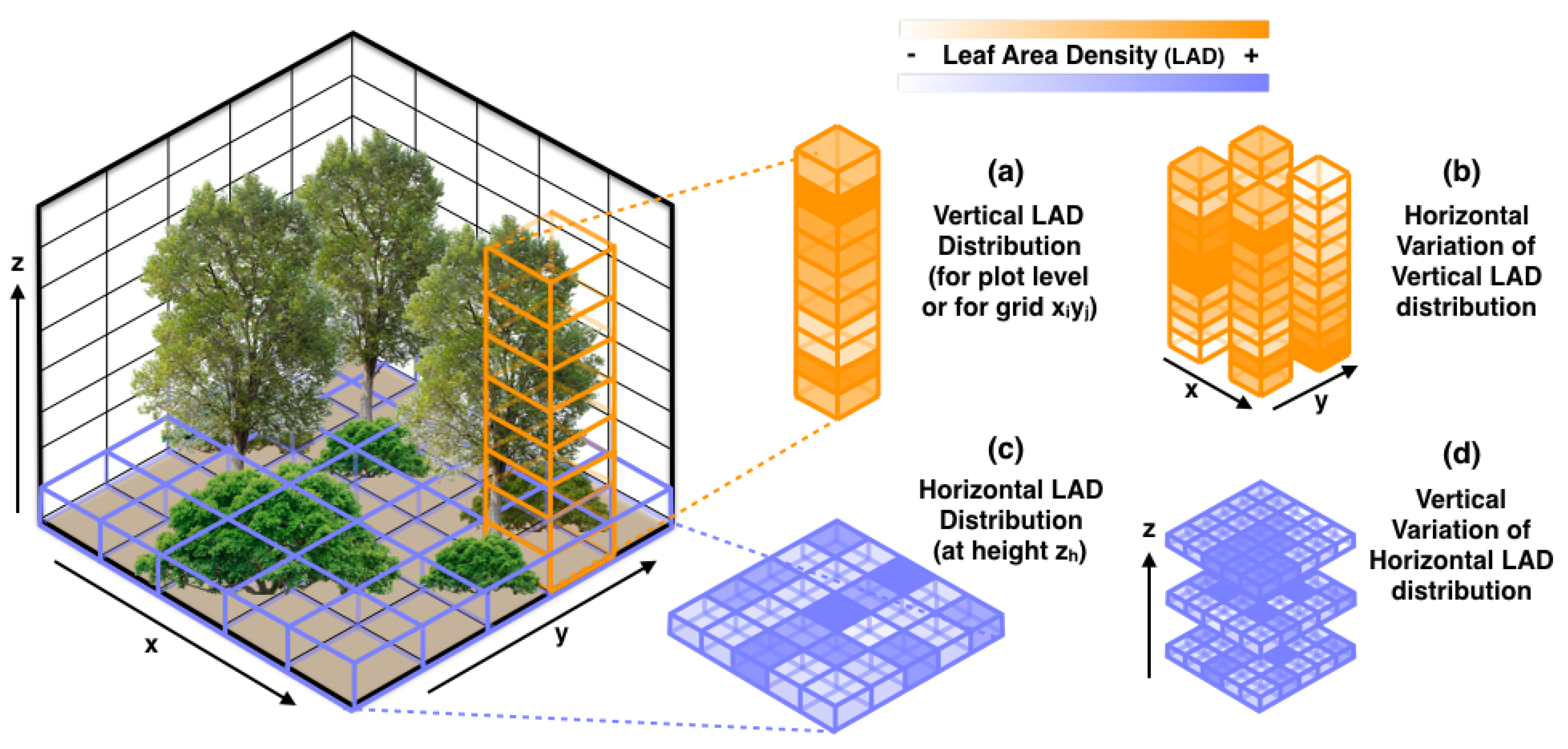
2.4.2. LAD-Based Metrics

To capture the 3D structural diversity that occurs below the top of the canopy, we used all lidar returns to estimate vegetation density at different height layers. Leaf area density (LAD), measured from lidar point-cloud data, is becoming a popular estimate of the total leaf area per unit of volume, as it can provide important information about the productivity and vertical structure of the forest [33]. LAD estimation relies on the concepts of leaf area index (LAI) and gap fraction (GF), which have been widely used in remote sensing studies of horizontal distribution of vegetation [34,35]. LAI represents the projected total surface area of leaves per unit ground surface area, while GF is interpreted as the light transmittance across a forest layer if a random leaf distribution is assumed [36]. The Beer–Lambert Law allows the measurement of LAI in terms of GF as:

$$LAI\left(z\right)=-\frac{ln\left(GF\right(z\left)\right)}{k},$$

(1)

where $GF\left(z\right)$ is the GF from the top of the canopy to the height z and k is an extinction coefficient [36]. When working with lidar data, the space can be divided into volumetric pixels (hereafter voxels) of height $\Delta z$, and $GF$ can be estimated by counting the number of returns above and below the target voxel i in a vertical column. We can define LAD for the voxel i as:

$$LA{D}_i=-\frac{ln\left(G{F}_i\right)}{k\Delta z};G{F}_i=-\frac{N_{be}}{N_{tot}{N}_{ab}},$$

(2)

where $N_{ab}$ is the number of lidar returns above the voxel, $N_{be}$ is the number of returns below the voxel, and $N_{tot}$ is the total number of returns in the vertical column [25]. Although a coefficient of extinction (k) of 0.5 has been assumed in some studies as a proxy to characterize the vegetation properties of many forest types [25,37], its value depends on the scale at which the LAD is measured and also on the lidar sensor properties. In this study, we used k values based on [23], who calibrated these values for the NEON lidar data at different scales, using field-based data calculations of the LAI and the GF.

We calculated the LAD for each 1 × l × l m voxel (where l = 20 or 40 m for vegetation plots and 200 m for bird plots, coinciding with the sampling dimensions of these plots) in each lidar plot. We derived two metrics to describe the vertical variation: the standard deviation, $sdlad=\sqrt{\frac{1}{H-1}{\sum }_{h=1}^H{(LA{D}_h-\overline{LAD})}^2}$, where H is the total number of height layers and $\overline{LAD}$ is the mean LAD across voxels, and the coefficient of variation, $cvlad=sdlad/\overline{LAD}$.

We built a second group of LAD-derived metrics in order to characterize the horizontal variation of the vertical vegetation profile. We divided every plot horizontally into smaller grids of 10 m × 10 m because this resolution is broad enough to obtain reliable LAD measurements [23] while providing enough grids to analyze the horizontal variation of the LAD distribution at a bird plot level (200 m × 200 m). However, due to the small size of the vegetation plots, 10 m × 10 m grids would have resulted in an insufficient amount of LAD vertical profiles to be able to estimate their horizontal variation. We used grids of 4 m × 4 m instead for the vegetation plots. We then calculated the LAD for each 1 m high interval at each grid (i.e., 10 m × 10 m × 1 m voxels in the case of bird plots), to obtain a LAD vertical profile at the grid level (see Figure 2a).

We calculated the mean LAD values across all voxels, $mlad=\frac{1}{IJH}{\sum }_{i=1}^I{\sum }_{j=1}^J{\sum }_{h=1}^{H}LA{D}_{ijh}$, where I and J are the number of grid cells along the x- and y-axes, respectively, and H is the number of height layers. Then, we used a Shannon entropy index [38] to characterize the LAD variation across all voxels. For the LAD Shannon entropy index, we first created LAD bins by calculating the range of LAD values for all plots and dividing by 50. Each bin represents a LAD range of equal width (e.g., LAD[0–0.05], LAD[0.5–0.10], etc.). Then, we assigned every voxel to a LAD bin. By doing this, the proportion of voxels that fall in each LAD bin can be calculated. We can define the LAD Shannon entropy index as:

$$shanlad=-\sum _{b=1}^{n_{bin}}{p}_{b}log\left(p_b\right),$$

(3)

where $p_b$ is the proportion of voxels assigned to a certain LAD bin b, for $p_b\ne 0$, and $n_{bin}$ is the total number of LAD bins. Higher LAD Shannon entropy index values represent higher heterogeneity of the distribution of vegetation density at the plot level.

We calculated coefficient of variation of the LAD vertical profile for each grid cell $ij$ ($LA{D}_{ij}$),

$$cvla{d}_{ij}=\frac{\sqrt{\frac{1}{H-1}{\sum }_{h=1}^H{(LA{D}_{ijh}-\overline{LA{D}_{ij}})}^2}}{\overline{LA{D}_{ij}}},$$

(4)

and then we obtained the mean values across all grid cells, $mcvlad=\frac{1}{IJ}{\sum }_{i=1}^I{\sum }_{j=1}^{J}cvla{d}_{ij}$. In addition, we calculated coefficient of variation of the mean LAD vertical profile across grid cells, $cvmlad=CV\left(mla{d}_{ij}\right)$, where $mla{d}_{ij}=\frac{1}{H}{\sum }_{h=1}^{H}LA{D}_{ijh}$ is the mean LAD across all voxels of grid cell $ij$, in order to characterize the horizontal variation of the vertical LAD distribution (Figure 2b). We then calculated a Shannon entropy index of the vertical LAD distribution of the voxels at the grid cell $ij$ ($shanla{d}_{ij}$). The mean $shanla{d}_{ij}$ across all grid cells ($mvershanlad=\frac{1}{IJ}{\sum }_{i=1}^I{\sum }_{j=1}^{J}shanla{d}_{ij}$) was calculated as a measure of mean vertical LAD heterogeneity.

Finally, we built metrics that estimated the horizontal LAD distribution at each height interval and their variation across height layers (Figure 2c,d). We calculated coefficient of variation of the LAD values across all voxels of a single height interval (for the whole plot),

$$horcvla{d}_h=\frac{\sqrt{\frac{1}{IJ-1}{\sum }_{i=1}^I{\sum }_{j=1}^J{(LA{D}_{ijh}-\overline{LA{D}_h})}^2}}{\overline{LA{D}_h}},$$

(5)

followed by calculation of their means across all height layers: $mhorcvlad=\frac{1}{H}{\sum }_{h=1}^{H}horcvla{d}_h$ Finally, we obtained a Shannon entropy index of the horizontal LAD distribution by first calculating the LAD values of all voxels of a plot at each height layer h. We assigned the LAD values of each voxel for that height to a LAD bin, and using the $shanlad$ equation, we calculated $shanla{d}_h$ to represent the heterogeneity of the horizontal distribution of vegetation densities at the plot level at each height layer h. The mean value of these measurements across all heights, $mhorshanlad=\frac{1}{H}{\sum }_{h=1}^{H}horshanla{d}_h$, is therefore the mean Shannon entropy index of the horizontal LAD distribution, which represents the average horizontal heterogeneity across canopy layers. A summary of the lidar-based metrics is shown in

Table 2. Description of the lidar-based metrics of forest structure.

Type	Variable	Description
First return	maxheight	Maximum height from first returns
	mheight	Mean height from first returns
	sdheight	Variation of height from first returns
Canopy model	mcanopy	Mean height from the canopy model
	sdcanopy	Variation of height from the canopy model
LAD—plot level	sdlad	Vertical variation of LAD
	cvlad	Vertical coefficient of variation of LAD
LAD—grid level	mlad	Mean LAD across all voxels
	shanlad	Shannon index of LAD variation across all voxels
	mcvlad	Mean vertical LAD coefficient of variation
	mhorcvlad	Mean horizontal LAD coefficient of variation
	cvmlad	Coefficient of variation of vertical LAD mean
	mhorshanlad	Mean Shannon index of horizontal LAD variation
	mvershanlad	Mean Shannon index of vertical LAD variation

.

2.5. Bird Species Richness

We used the breeding landbird point counts the (BLPC) dataset [39] from NEON to model the influence of the lidar-derived metrics on bird species richness. This dataset provides records of identification of landbird species associated with terrestrial habitats [40]. The surveying methods are based on point counts, with one or more experienced observers standing at a central point for six minutes. During that period, every species heard or seen within a 125 m radius is recorded. Surveys provide grids of nine point counts at several randomized sampled locations within a site. However, for smaller sites where nine-point grids cannot be allocated, single points are randomly sampled across the site. In our study, we only used the central point count of the nine point grid, enabling the comparison between points at different sites. By including only one point count per sample location, we also minimized spatial autocorrelation between observations. For the points where the survey was performed more than once within a year, we only used the first survey. We used data for the 2016 breeding season for all studied sites, except for the SERC site, for which we used 2017 data due to the lack of point counts in 2016. We used a total of 61 points that coincided spatially with available lidar data in 2016. The number of points for each of the sites can be seen in Table 1. We used bird richness, which is defined as the number of different species identified at each point count, as the response variable in the random forests’ models.

2.6. Statistical Analysis

We compared the lidar-derived metrics, calculated for the woody plant vegetation structure (WPVS) plots, with the variation in the three field-based vegetation structure metrics: height, stem diameter, and crown diameter. We calculated the Pearson correlation coefficients between the standard deviation of the field-based metrics and the lidar metrics.

We then calculated the lidar-derived metrics for the bird plots. We also extracted mean annual temperature values for each bird plot, in order to analyze the relationship between this variable and the studied metrics, as well as to estimate its differential effects on bird richness. We extracted the average monthly mean temperature values for 1970–2000 from the WorldClim database [41] and calculated a yearly temperature average. We used lidar-derived metrics together with temperature (expressed as ${}^{\circ }\mathrm{C}$ × 100) as explanatory variables of bird richness. First, in order to evaluate the relationships between the explanatory variables, we calculated bivariate Pearson correlation coefficients. To visualize the similarity between pairs and groups of variables, we performed hierarchical clustering using Pearson correlation coefficients as the pairwise distance metric ($d_{ab}=1-r_{ab}$, where $d_{ab}$ is the pairwise distance between variables a and b and $r_{ab}$ is the Pearson correlation coefficient between variables a and b) using the hclust function in R.

We built random forests (RF, [42]) regression models to analyze the ability of the lidar-derived metrics to explain bird species richness variability across plots. Often, RF models are used to address complex variable interactions [42,43] and they are becoming a popular method to study the shapes of ecological responses against predictors [44,45]. We built several RF regression models using 500 trees with different sets of predictor variables. We created one model using only the canopy height metrics as predictors. We created two models using the LAD-based metrics: one with all LAD-based metrics and another using only LAD grid-based metrics (see Table 2). We finally created two more models using a parsimonious subset of predictors, based on their predictive power (see below). We ran each model 100 times and averaged the variance explained and the variable importance measurements because the results of an RF model can differ slightly every time they are performed.

We used the mean decrease in accuracy (MDA, [42]) index to evaluate the relative importance of each predictor on the explanatory power of the models. The MDA index uses the left-out data samples at each regression tree (out-of-bag data), estimating the average difference in the model accuracy when the focal predictor is randomly permuted at each tree. We used feature selection for two of the models in order to reduce the complexity and collinearity between explanatory variables, which might affect the analysis on the response-shape analysis. We performed feature selection using a stepwise process, where a model that includes all variables is created and the variable ranked least in importance is recursively dropped, until the accuracy of the variable-reduced model starts to rapidly decrease [46]. Finally, we used RF feature contribution analysis [47] to elucidate how model predictors affect bird species richness. The feature contribution measures the average increase in the response variable after a tree-node split that used the studied variable. The intensity and direction of the effect on the response variable can be visualized by plotting the feature contribution against the explanatory variable’s value.

3. Results

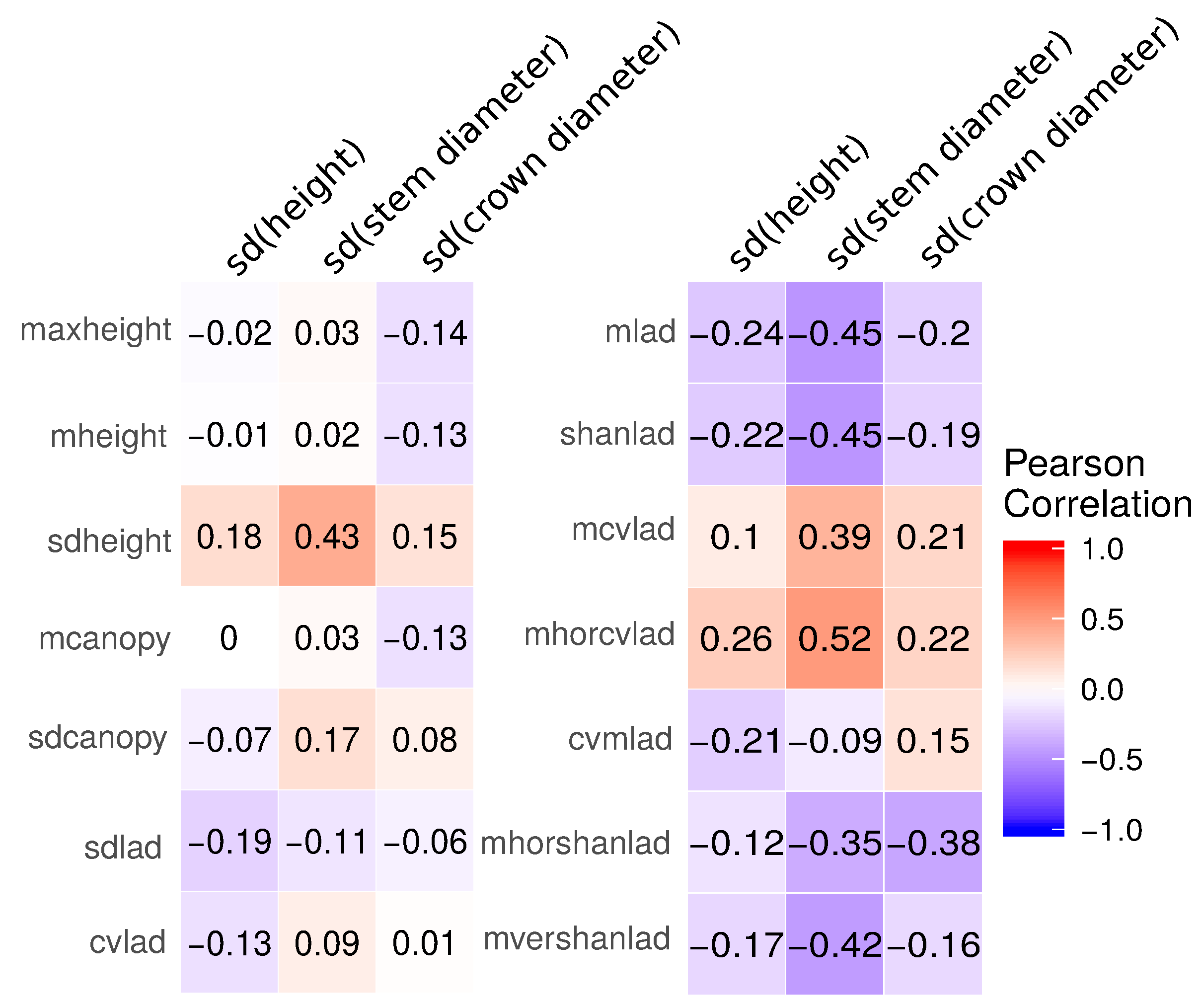
3.1. Field-Based Vegetation Structure and Lidar-Derived Metrics

We calculated lidar-derived metrics of vegetation structural heterogeneity for the woody plant vegetation structure plots (WPVS, Supplementary Materials, Table S1) and analyzed the correlations between those and the standard deviation of the three field-based structural variables. In general, lidar-derived metrics and field-based measurements were only weakly to moderately correlated (Figure 3). The strongest positive correlations (Pearson coefficient = 0.39 to 0.52) were found between the standard deviation of stem diameter and the standard deviation in the canopy height ($sdheight$), as well as the mean vertical and horizontal coefficient of variation of LAD ($mcvlad$ and $mhorcvlad$). We found negative correlations (Pearson coefficient = −0.42 to −0.45) between the standard deviation of stem diameter and Shannon index of LAD variation across all voxels ($shanlad$), mean LAD across all voxels ($mlad$), and mean Shannon index of vertical LAD variation ($mvershanlad$).

3.2. Bird Plots

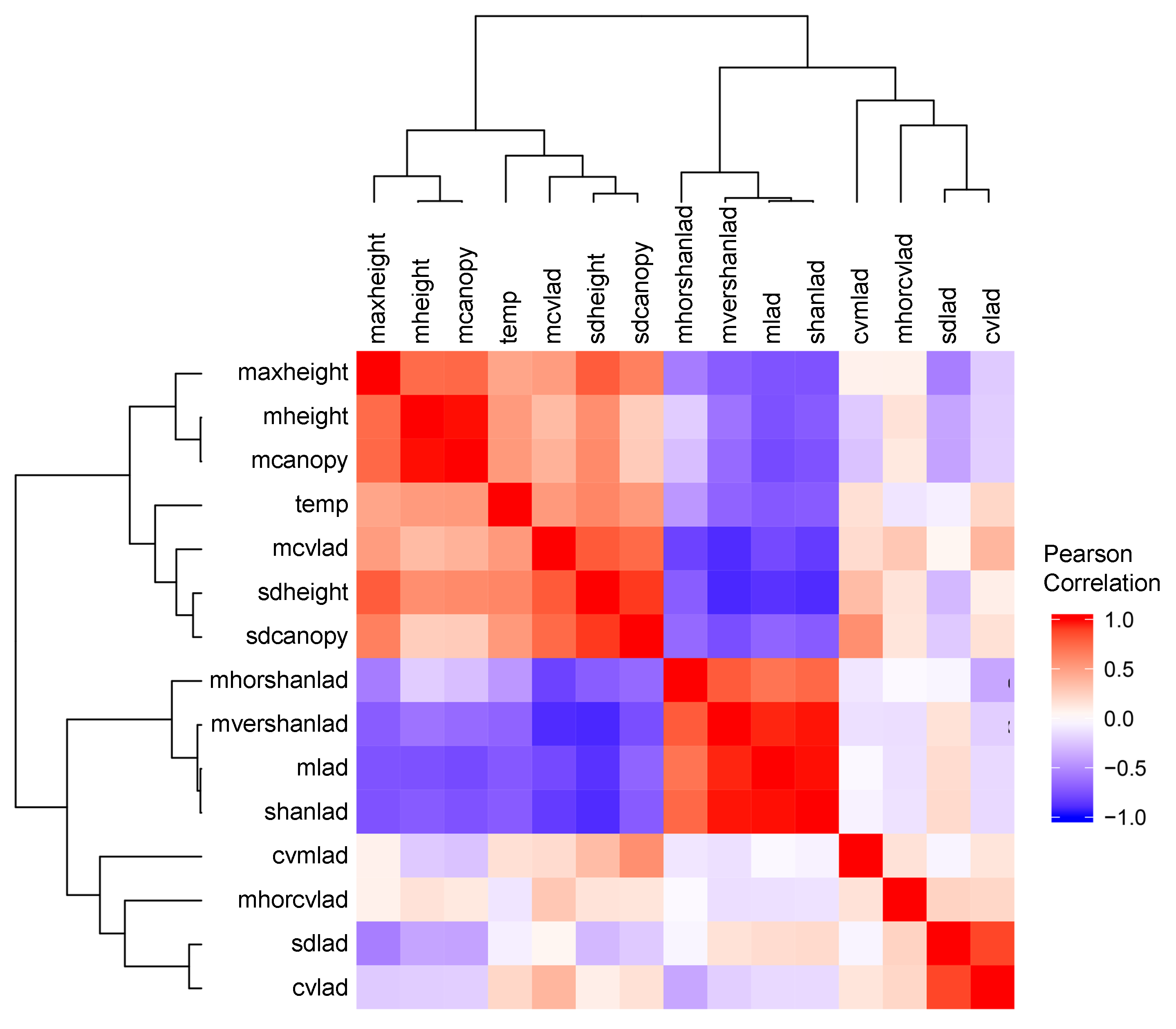
3.2.1. Lidar-Derived Metrics

We examined relationships among lidar metrics (Supplementary Materials, Table S2) and mean annual temperature at the bird-plot level via correlation matrix (Supplementary Materials, Table S3) and hierarchical clustering analysis. The correlation matrix heatmap shows strong correlations (positive and negative) between variables, and the dendrogram from the hierarchical clustering analysis shows variable clustering in addition to the dissimilarities between variables and clusters of variables (Figure 4).

The dendrogram revealed three main clusters of variables. In the first strong cluster delineated by the left main branch, there were strong moderate-to-positive correlations between seven variables that include canopy height metrics ($maxheight$, $mheight$, $mcanopy$), canopy height variation metrics ($sdheight$, $sdcanopy)$, a metric representing vertical variation in LAD ($mcvlad$), and annual mean temperature ($temp$). Within this cluster, the canopy height metrics and canopy height variation metrics formed clear individual sub-clusters. The second main cluster (left sub-branch of the right main branch) included three strongly, positively correlated variables [mean LAD ($mlad$), Shannon index of LAD across all voxels ($shanlad$), and mean Shannon index of vertical diversity ($mvershanlad$)] and a fourth variable, mean Shannon index of horizontal diversity ($mhorshanlad$) that had a moderate positive correlation with the first three variables. In general, variables in this cluster showed moderate-to-strong negative correlations with variables in the first cluster. The right cluster of the right main branch of the dendrogram comprised two highly correlated variables, $sdlad$ and $cvlad$, both measuring vertical LAD heterogeneity at the plot level, along with $cvmlad$ and $mhorcvlad$, the horizontal variation of the LAD. The latter two variables showed little association with the former two as indicated by the low correlation values and high branch lengths in the dendrogram.

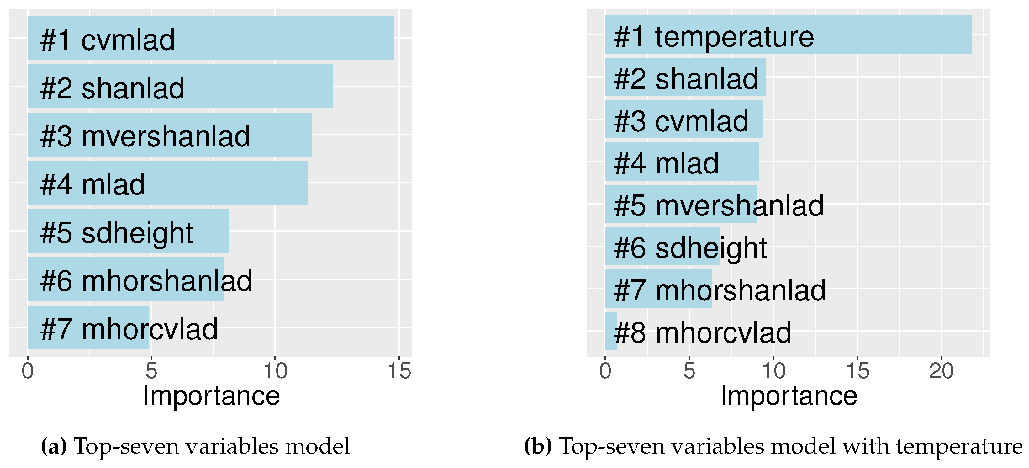
3.2.2. Bird Species Richness Models

Different combinations of explanatory variables were used to create RF models of bird species richness followed by calculation of model accuracy (

Table 3. Accuracy of the random forests (RF) models for bird species’ richness.

Model	Variables	Variance Explained (%)
Top-seven variables	cvmlad, shanlad, mvershanlad, mlad, sdheight, mhorshanlad, mhorcvlad	43.82
Top-seven + temperature	cvmlad, shanlad, mvershanlad, sdheight, mlad, mhorshanlad, mhorcvlad, temperature	61.34
Top of canopy	maxheight, mheight, sdheight, mcanopy, sdcanopy	32.10
LAD-derived	All LAD derived variables (see Table 2)	44.41
LAD-derived (grid based)	All LAD grid based variables (see Table 2)	42.71

). Models using only LAD-derived metrics had greater explanatory power than those models using only top-of-the-canopy metrics. Models that used only grid-based LAD metrics were almost as accurate as those using all LAD-derived metrics (42.7% versus 44.4%, respectively). Recursive dropping of the least important variables allowed the creation of a parsimonious, variable-reduced model (hereafter, ‘top-seven variables model’). This enabled collinearity and model complexity to be reduced, a fundamental aspect for model analysis (e.g., response shapes), while maintaining high accuracy. This variable-reduced model included the seven most important predictor variables and explained 43.8% of variance. The model included one variable related to the canopy ($sdheight$), one related to vegetation density ($mlad$), and five variables representing horizontal ($cvmlad$, $mhorcvlad$, $mhorshanlad$), vertical ($mvershanlad$), and overall vegetation structural heterogeneity ($shanlad$). Adding mean annual temperature to this model increased the explained variance by 17.5%.

The variable importance ranking, measured by the MDA, was studied for the top-seven variables model (Figure 5a). The most important variable for explaining bird richness was $cvmlad$, followed by $shanlad$. The $cvmlad$ metric measures the horizontal variation of the mean vertical LAD, while $shanlad$ is a measure of the LAD heterogeneity across all voxels. One metric that primarily represents the vertical component of the LAD heterogeneity ($mvershanlad$) was ranked 3rd, while $mlad$, a measure of overall vegetation density, was ranked 4th. One metric related to canopy height, $sdheight$, was included in the model, although it had lower importance than all but two LAD-derived metrics, $mhorshanlad$ and $mhorcvlad$, which measure mean horizontal LAD heterogeneity. We reanalyzed variable importance after adding mean annual temperature to the top-seven variables model. Temperature was the most important variable for explaining bird richness, with almost 15 MDA score units higher than the second ranked variable (Figure 5b). There were also small changes in variable importance ranking among lidar-derived metrics: $shanlad$ became the most important lidar-derived metric, followed by $cvmlad$ and $mlad$.

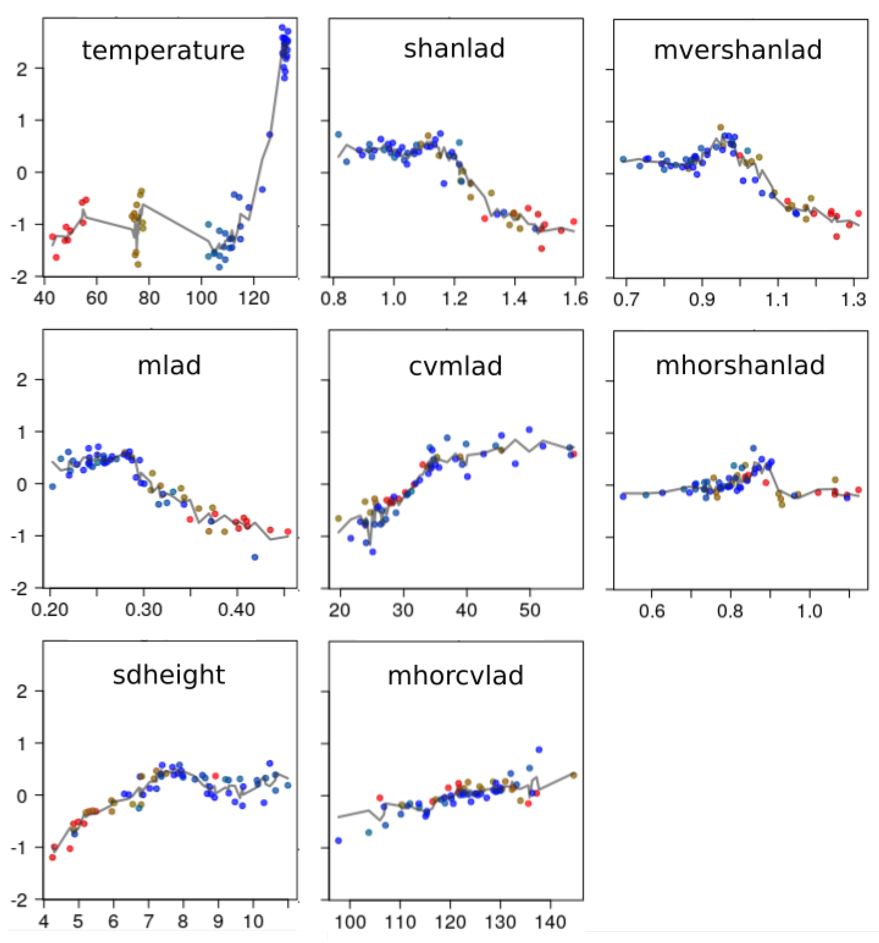
3.2.3. Shapes of Bird Richness Response

The feature contribution analysis revealed disparate (and often nonlinear) responses of bird species richness to the different predictor variables (Figure 6). Mean annual temperature was nonlinearly and sharply associated with bird richness. Richness changed very little with an increase in temperature from ≈4–11.5${}^{\circ }\mathrm{C}$. However, there was a rapid increase in richness as temperature increased beyond ≈$11.5{}^{\circ }\mathrm{C}$ (point counts conducted at the SERC site). Like mean annual temperature, many of the lidar-derived vegetation structure metrics demonstrated nonlinear effects on bird richness; however, these metrics did not appear to affect richness as strongly as mean annual temperature, consistent with variable importance rankings.

Bird richness increased with metrics that captured the horizontal LAD heterogeneity, $cvmlad$, $mhorshanlad$, and $mhorcvlad$, with the increase being steeper from low to moderate heterogeneity and saturating at moderate to high heterogeneity.

Conversely, the Shannon index-based metric that represents overall LAD heterogeneity ($shanlad$), the Shannon index-based vertical LAD heterogeneity metric ($mvershanlad$), and the mean LAD metric ($mlad$) showed no-to-weak positive effects at low to intermediate values followed by strong negative effects going from moderate to high values. The metric related to the variation of the canopy height, $sdheight$, showed an increasing positive effect on bird richness which saturated at around intermediate canopy height variation.

The response patterns for metrics excluded from the top-seven variables are presented in Figure S4, Supplementary Material.

4. Discussion

Discrete lidar is becoming an effective tool to study forest structure, but creating lidar-derived metrics that reliably characterize the vegetation heterogeneity in 3D is challenging. Our findings suggest that identifying appropriate lidar metrics that account for the different aspects of structural heterogeneity can provide new insights into structural heterogeneity-biodiversity studies. Metrics based on LAD measurements showed better explanatory power with regard to bird richness than those based on the variation of canopy heights. Our results also show how vertical and horizontal heterogeneity can have disparate effects on bird richness.

Our lidar metrics were weakly to moderately correlated with field-based measurements of vegetation structure. Among the latter, variation in stem diameter was most strongly correlated with lidar metrics. Previous studies had shown stronger correlations between lidar-derived vegetation metrics and field-based measurements [13,48,49,50]. However, most of these studies examined lidar metrics that were unrelated to heterogeneity, such as aboveground biomass, or used spatially located individuals to represent the horizontal distribution of the vegetation in the field. In our study, the weak relationships between lidar metrics and field heterogeneity measurements are likely largely due to mismatches between aspects of heterogeneity quantified by the two types of measurements. For example, data on the heights were not assigned to individual tree crowns, limiting our assessment of metrics related to vertical heterogeneity. Furthermore, the field data comprised many vegetation types ranging from large trees to small bushes; therefore, consideration of the total variation in heights or stem diameter could have caused misleading measurements of vegetation heterogeneity. For instance, large trees might have had the biggest impact on some of the lidar-derived metrics, while the field-based measurements might have heavily weighted the most common individuals such as small bushes or small trees. Future work linking the spatial location of the individuals with the structural measurements are needed to create field-based spatially explicit models of the distribution of the vegetation and to study their relationships with the lidar metrics.

In our study, we used metrics based on LAD measurements as explanatory variables of bird richness across forest plots. To the best of our knowledge, this is the first time these metrics have been used to study the relationships between forest structural heterogeneity and animal diversity. Mean LAD values for the 10 m × 10 m × 1 m voxels were within the ranges of those obtained in previous work that estimated LAD in the SERC site using lidar data [23] or field measurements [51]. Mean LAD was closely and positively related to metrics capturing the vertical structural heterogeneity, but did not have a strong relationship with other metrics representing horizontal heterogeneity. Temperature was also closely related to some of the LAD metrics, and, surprisingly, plots with higher temperatures presented lower LAD densities and lower vertical heterogeneity. Although temperature gradients have been linked to differences in forest biomass [52], these relationships are strongly influenced by the scale of the studies and forest type, while other climatic factors, such as water deficit, may have strong effects at regional scales [53]. In general, metrics that aimed to capture vertical heterogeneity, albeit built with diverse methods, showed close inter-relationships and the same can be said for the horizontal heterogeneity metrics. Despite their reliability, LAD-based metrics present several limitations. For example, the light attenuation coefficient k could vary slightly between forests with different tree compositions [25], while specific k values must be estimated for different sensors and plot extents [23,24]. LAD values at the lower canopy layers may also be overestimated for low-density point lidar sensors such as NEON’s [23]. Differences in point densities within a plot, owing to differences in lidar coverage (simple or double flight pass) could also affect LAD measurements for small voxels, such as those created for the vegetation plots, because the dependency of LAD values on point density becomes significant for scales smaller than 10 m × 10 m [23]. Lidar scan angle might also affect GP and LAI measurements for single coverage regions [54,55]. Despite the fact that effects of low angles (single coverage regions generally present low angles) on GP and LAI were shown to be minimal [54], the influence of the scan angle could depend on the forest type [56]. Corrections of these possible biases should be addressed in the future.

LAD-based metrics showed, in general, higher explanatory power with regard to bird richness than metrics based on top of the canopy measurements. Models based on LAD metrics alone were found to be more accurate than canopy-based metrics, and LAD metrics were found to be more important than canopy-based metrics in the mixed-metrics models. Standard variation of the canopy height was nonetheless included as the fifth most important variable in the the top-seven variables model. Metrics based on canopy height have long been found to be correlated with species distributions or diversity of many taxa [5]. Despite very early work linking the distribution of biodiversity with vertical vegetation heterogeneity [1,2], canopy-based metrics are most commonly used in studies linking habitat structure to animal ecology [14]. This is probably because these metrics can be easily extracted from satellite data or from lidar sensors with minimal data processing and with high reliability. In this study, metrics that accounted for the horizontal variation across 10 m × 10 m grids had better explanatory power with regard to bird richness than those metrics measuring the vertical heterogeneity at the plot level. A few animal ecology studies considered the horizontal variation of the vertical forest structure [57,58], finding that this horizontal component was key for explaining species distributions. However, most studies that measured structural heterogeneity using vertical vegetation profiles did not consider the horizontal component [5,13,14,17]. The capabilities of the new airborne lidar sensors in terms of pulse density and extent should allow ecologists to study the variation of the vertical vegetation profiles with greater detail [59]. Grid-based metrics such as the ones built in this study will enable the addition of this horizontal component to structural heterogeneity-biodiversity studies.

The analysis of the models’ response shapes revealed different components of structural heterogeneity affected bird richness disparately. Metrics measuring horizontal heterogeneity at different canopy layers, or measuring the horizontal variation of the vertical canopy profile, showed positive effects on bird richness. While the positive effects of horizontal structural heterogeneity on bird richness are well documented [3,60,61], very few of those studies considered all three dimensions of the vegetation (but see [6]). This study did not consider, however, the effects of differences in forest types between sites. The intensity and shape of the effect of horizontal heterogeneity could differ between forests with different vertical configurations, therefore future research considering horizontal heterogeneity across a variety of forest types will help clarifying the absolute effects of this factor on bird richness. The horizontal variation of the mean vertical LAD showed a strong positive effect on bird richness, similar to the effect of canopy height variation. Therefore, variation in canopy height and canopy cover may be closely linked to horizontal heterogeneity in lower canopy layers, which might explain the success of studies that used canopy metrics to explain bird distributions [62].

While lower and intermediate values of vertical heterogeneity showed positive effects on bird richness, our analyses indicate that high vertical heterogeneity had a detrimental effect. These results contradict previous studies that found higher bird diversity with increased vertical profile heterogeneity [1,5,17,63]. However, vertical heterogeneity in many of those studies was calculated using only canopy height variations, or with metrics that did not consider all canopy height layers. The Shannon entropy index has also been used to characterize the vertical distribution of vegetation. For example, Refs. [1,64] used a Shannon entropy index to study the foliage height diversity, but the index was calculated as the evenness of the vegetation density across height layers and not as vegetation density heterogeneity across heights. However, Ref. [17] used full waveform lidar data to create an entropy index similar to our $mvershanlad$ metric, finding positive associations with a single songbird species. Other studies found negative associations between vertical heterogeneity and bird richness [16], supporting our results. Nevertheless, we acknowledge that the relationship between vertical heterogeneity and diversity may be highly dependent on how heterogeneity is measured. Our vertical heterogeneity metric based on Shannon-index is strongly correlated with the Shannon-index of overall heterogeneity and mean vegetation density, thus adding difficulties to the isolation and study of this structural factor. Further work is needed to develop and examine vertical heterogeneity metrics that are independent of other structural metrics to test the effect of vertical heterogeneity more conclusively.

Besides the nonlinearity and correlations between components of forest structural heterogeneity, some components may be correlated to other forest characteristics that affect bird diversity, such as forest successional stage [65] and fire disturbance [66]. Structural heterogeneity–diversity relationships might also be height- and taxa-dependent, as some bird groups prefer highly dense and homogeneous lower canopy layers, while other groups may rely only on the heterogeneity of the upper layers [6]. Variation in bird detectability from point counts could also affect the study of forest structural heterogeneity–diversity. Different bird species can be heard from much farther away than others and the same individual of a species can be heard from different distances depending on the forest type [67]. Denser canopies could decrease the detectability of some bird species, thereby possibly contributing to the negative correlations between bird richness and vegetation density observed in our study. Further work to correct this bias is needed.

5. Conclusions

The increasing capabilities and availability of lidar data allow researchers to characterize forest structure with higher detail. In this study, we developed lidar-derived metrics to analyze structural heterogeneity across forests from the east and northeastern US. We demonstrated the utility of these metrics in explaining bird species richness at 61 point counts distributed across these forests. We found that metrics based on LAD measurements better explained bird species richness than metrics relying on the variation of canopy height. Dividing the forest plots into smaller grids allowed us to not only study the vertical component of the structural heterogeneity, but also its horizontal variation below the top of the canopy, while enabling analysis of how the vegetation density is horizontally distributed within the plot. Bird richness was enhanced by horizontal heterogeneity, whereas high vertical heterogeneity showed negative effects, contrary to previous research that studied vegetation vertical profiles. Although further research is needed to determine how these results might vary for different forest types, our findings highlight the need for structure–animal diversity models to incorporate metrics that capture the vegetation heterogeneity in different dimensions.

References

1. MacArthur, R.H.; MacArthur, J.W. On bird species diversity. Ecology 1961, 42, 594–598. [Google Scholar] [CrossRef]
2. Lack, D. The numbers of bird species on islands. Bird Study 1969, 16, 193–209. [Google Scholar] [CrossRef] [Green Version]
3. Tews, J.; Brose, U.; Grimm, V.; Tielbörger, K.; Wichmann, M.; Schwager, M.; Jeltsch, F. Animal species diversity driven by habitat heterogeneity/diversity: The importance of keystone structures. J. Biogeogr. 2004, 31, 79–92. [Google Scholar] [CrossRef]
4. Bramer, I.; Anderson, B.J.; Bennie, J.; Bladon, A.J.; De Frenne, P.; Hemming, D.; Hill, R.A.; Kearney, M.R.; Körner, C.; Korstjens, A.H.; et al. Advances in Monitoring and Modelling Climate at Ecologically Relevant Scales. Adv. Ecol. Res. 2018, 58, 101–161. [Google Scholar]
5. Bergen, K.; Goetz, S.; Dubayah, R.; Henebry, G.; Hunsaker, C.; Imhoff, M.; Nelson, R.; Parker, G.; Radeloff, V. Remote sensing of vegetation 3-D structure for biodiversity and habitat: Review and implications for lidar and radar spaceborne missions. J. Geophys. Res. Biogeosci. 2009, 114. [Google Scholar] [CrossRef]
6. Vogeler, J.C.; Hudak, A.T.; Vierling, L.A.; Evans, J.; Green, P.; Vierling, K.T. Terrain and vegetation structural influences on local avian species richness in two mixed-conifer forests. Remote Sens. Environ. 2014, 147, 13–22. [Google Scholar] [CrossRef]
7. Hinsley, S.A.; Hill, R.A.; Bellamy, P.E.; Balzter, H. The Application of Lidar in Woodland Bird Ecology. Photogramm. Eng. Remote Sens. 2006, 72, 1399–1406. [Google Scholar] [CrossRef]
8. Müller, J.; Stadler, J.; Brandl, R. Composition versus physiognomy of vegetation as predictors of bird assemblages: The role of lidar. Remote Sens. Environ. 2010, 114, 490–495. [Google Scholar] [CrossRef]
9. Müller, J.; Brandl, R.; Buchner, J.; Pretzsch, H.; Seifert, S.; Strätz, C.; Veith, M.; Fenton, B. From ground to above canopy—Bat activity in mature forests is driven by vegetation density and height. For. Ecol. Manag. 2013, 306, 179–184. [Google Scholar] [CrossRef]
10. Gouveia, S.F.; Villalobos, F.; Dobrovolski, R.; Beltrão-Mendes, R.; Ferrari, S.F. Forest structure drives global diversity of primates. J. Anim. Ecol. 2014, 83, 1523–1530. [Google Scholar] [CrossRef] [PubMed] [Green Version]
11. Shine, R.; Barrott, E.G.; Elphick, M.J. Some like it hot: Effects of forest clearing on nest temperatures of montane reptiles. Ecology 2002, 83, 2808–2815. [Google Scholar] [CrossRef]
12. Müller, J.; Bae, S.; Röder, J.; Chao, A.; Didham, R.K. Airborne LiDAR reveals context dependence in the effects of canopy architecture on arthropod diversity. For. Ecol. Manag. 2014, 312, 129–137. [Google Scholar] [CrossRef]
13. Listopad, C.M.; Masters, R.E.; Drake, J.; Weishampel, J.; Branquinho, C. Structural diversity indices based on airborne LiDAR as ecological indicators for managing highly dynamic landscapes. Ecol. Indic. 2015, 57, 268–279. [Google Scholar] [CrossRef]
14. Davies, A.B.; Asner, G.P. Advances in animal ecology from 3D-LiDAR ecosystem mapping. Trends Ecol. Evolut. 2014, 29, 681–691. [Google Scholar] [CrossRef]
15. Simonson, W.D.; Allen, H.D.; Coomes, D.A. Applications of airborne lidar for the assessment of animal species diversity. Methods Ecol. Evolut. 2014, 5, 719–729. [Google Scholar] [CrossRef] [Green Version]
16. Goetz, S.; Steinberg, D.; Dubayah, R.; Blair, B. Laser remote sensing of canopy habitat heterogeneity as a predictor of bird species richness in an eastern temperate forest, USA. Remote Sens. Environ. 2007, 108, 254–263. [Google Scholar] [CrossRef]
17. Goetz, S.J.; Steinberg, D.; Betts, M.G.; Holmes, R.T.; Doran, P.J.; Dubayah, R.; Hofton, M. Lidar remote sensing variables predict breeding habitat of a Neotropical migrant bird. Ecology 2010, 91, 1569–1576. [Google Scholar] [CrossRef] [Green Version]
18. Stein, A.; Gerstner, K.; Kreft, H. Environmental heterogeneity as a universal driver of species richness across taxa, biomes and spatial scales. Ecol. Lett. 2014, 17, 866–880. [Google Scholar] [CrossRef] [PubMed] [Green Version]
19. De Araújo, W.S. Different relationships between galling and non-galling herbivore richness and plant species richness: A meta-analysis. Arthropod-Plant Interact. 2013, 7, 373–377. [Google Scholar] [CrossRef]
20. Richter, K.; Stelling, N.; Maas, H. Correcting attenuation effects caused by interactions in the forest canopy in full-waveform airborne laser scanner data. Int. Arch. Photogramm. Remote Sens. Spat. Inf. Sci. 2014, 40, 273. [Google Scholar] [CrossRef]
21. Weiss, M.; Baret, F.; Smith, G.; Jonckheere, I.; Coppin, P. Review of methods for in situ leaf area index (LAI) determination: Part II. Estimation of LAI, errors and sampling. Agric. For. Meteorol. 2004, 121, 37–53. [Google Scholar] [CrossRef]
22. Waring, R.H. Estimating forest growth and efficiency in relation to canopy leaf area. Adv. Ecol. Res. 1983, 13, 327–354. [Google Scholar]
23. Kamoske, A.G.; Dahlin, K.M.; Stark, S.C.; Serbin, S.P. Leaf area density from airborne LiDAR: Comparing sensors and resolutions in a temperate broadleaf forest ecosystem. For. Ecol. Manag. 2019, 433, 364–375. [Google Scholar] [CrossRef]
24. Almeida, D.R.A.d.; Stark, S.C.; Shao, G.; Schietti, J.; Nelson, B.W.; Silva, C.A.; Gorgens, E.B.; Valbuena, R.; Papa, D.d.A.; Brancalion, P.H.S. Optimizing the Remote Detection of Tropical Rainforest Structure with Airborne Lidar: Leaf Area Profile Sensitivity to Pulse Density and Spatial Sampling. Remote Sens. 2019, 11, 92. [Google Scholar] [CrossRef]
25. Bouvier, M.; Durrieu, S.; Fournier, R.A.; Renaud, J.P. Generalizing predictive models of forest inventory attributes using an area-based approach with airborne LiDAR data. Remote Sens. Environ. 2015, 156, 322–334. [Google Scholar] [CrossRef]
26. White, J.C.; Coops, N.C.; Wulder, M.A.; Vastaranta, M.; Hilker, T.; Tompalski, P. Remote sensing technologies for enhancing forest inventories: A review. Can. J. Remote Sens. 2016, 42, 619–641. [Google Scholar] [CrossRef]
27. Kampe, T.U.; Johnson, B.R.; Kuester, M.A.; Keller, M. NEON: The first continental-scale ecological observatory with airborne remote sensing of vegetation canopy biochemistry and structure. J. Appl. Remote Sens. 2010, 4, 043510. [Google Scholar] [CrossRef]
28. National Ecological Observatory Network. Data Product NEON.DOM.SITE.DP1.10098.001; Battelle: Boulder, CO, USA, 2016; Available online: http://data.neonscience.org (accessed on 20 January 2019).
29. National Ecological Observatory Network. Data Product NEON.DOM.SITE.DP1.30003.001; Battelle: Boulder, CO, USA, 2016; Available online: http://data.neonscience.org (accessed on 1 November 2018).
30. Roussel, J.; Auty, D. lidR: Airborne LiDAR Data Manipulation and Visualization for Forestry Applications. 2018. Available online: https://rdrr.io/cran/lidR/ (accessed on 15 January 2019).
31. R Development Core Team. R: A Language and Environment for Statistical Computing; R Foundation for Statistical Computing: Vienna, Austria, 2013. [Google Scholar]
32. Hijmans, R. Raster: Geographic Analysis and Modeling with Raster Data, 2nd ed.; R Foundation for Statistical Computing: Vienna, Austria, 2010; pp. 1–204. Available online: https://CRAN.R-project.org/package=raster (accessed on 15 December 2018).
33. Detto, M.; Asner, G.P.; Muller-Landau, H.C.; Sonnentag, O. Spatial variability in tropical forest leaf area density from multireturn lidar and modeling. J. Geophys. Res. Biogeosci. 2015, 120, 294–309. [Google Scholar] [CrossRef] [Green Version]
34. Jonckheere, I.; Fleck, S.; Nackaerts, K.; Muys, B.; Coppin, P.; Weiss, M.; Baret, F. Review of methods for in situ leaf area index determination: Part I. Theories, sensors and hemispherical photography. Agric. For. Meteorol. 2004, 121, 19–35. [Google Scholar] [CrossRef]
35. Hopkinson, C.; Lovell, J.; Chasmer, L.; Jupp, D.; Kljun, N.; van Gorsel, E. Integrating terrestrial and airborne lidar to calibrate a 3D canopy model of effective leaf area index. Remote Sens. Environ. 2013, 136, 301–314. [Google Scholar] [CrossRef]
36. Bréda, N.J. Ground-based measurements of leaf area index: a review of methods, instruments and current controversies. J. Exp. Bot. 2003, 54, 2403–2417. [Google Scholar] [CrossRef] [PubMed] [Green Version]
37. Tang, H.; Brolly, M.; Zhao, F.; Strahler, A.H.; Schaaf, C.L.; Ganguly, S.; Zhang, G.; Dubayah, R. Deriving and validating Leaf Area Index (LAI) at multiple spatial scales through lidar remote sensing: A case study in Sierra National Forest, CA. Remote Sens. Environ. 2014, 143, 131–141. [Google Scholar] [CrossRef]
38. Pluim, J.P.; Maintz, J.A.; Viergever, M.A. Mutual-information-based registration of medical images: A survey. IEEE Trans. Med. Imaging 2003, 22, 986–1004. [Google Scholar] [CrossRef] [PubMed]
39. National Ecological Observatory Network. Data Product NEON.DOM.SITE.DP1.10003.001; Battelle: Boulder, CO, USA, 2016; Available online: http://data.neonscience.org (accessed on 20 January 2019).
40. Ralph, C.J.; Geupel, G.R.; Pyle, P.; Martin, T.E.; DeSante, D.F. Handbook of Field Methods for Monitoring Landbirds; USDA Forest Service/UNL Faculty Publications: Berkeley, CA, USA, 1993; p. 105.
41. Hijmans, R.J.; Cameron, S.E.; Parra, J.L.; Jones, P.G.; Jarvis, A. Very high resolution interpolated climate surfaces for global land areas. Int. J. Climatol. 2005, 25, 1965–1978. [Google Scholar] [CrossRef] [Green Version]
42. Breiman, L. Random forests. Mach. Learn. 2001, 45, 5–32. [Google Scholar] [CrossRef]
43. Prasad, A.M.; Iverson, L.R.; Liaw, A. Newer classification and regression tree techniques: Bagging and random forests for ecological prediction. Ecosystems 2006, 9, 181–199. [Google Scholar] [CrossRef]
44. Cutler, D.R.; Edwards, T.C., Jr.; Beard, K.H.; Cutler, A.; Hess, K.T.; Gibson, J.; Lawler, J.J. Random forests for classification in ecology. Ecology 2007, 88, 2783–2792. [Google Scholar] [CrossRef]
45. Carrasco, L.; Mashiko, M.; Toquenaga, Y. Application of random forest algorithm for studying habitat selection of colonial herons and egrets in human-influenced landscapes. Ecol. Res. 2014, 29, 483–491. [Google Scholar] [CrossRef] [Green Version]
46. Genuer, R.; Poggi, J.M.; Tuleau-Malot, C. Variable selection using random forests. Pattern Recognit. Lett. 2010, 31, 2225–2236. [Google Scholar] [CrossRef] [Green Version]
47. Palczewska, A.; Palczewski, J.; Robinson, R.M.; Neagu, D. Interpreting random forest classification models using a feature contribution method. Integr. Reusable Syst. 2014, 193–218. [Google Scholar]
48. Asner, G.P.; Mascaro, J.; Muller-Landau, H.C.; Vieilledent, G.; Vaudry, R.; Rasamoelina, M.; Hall, J.S.; Van Breugel, M. A universal airborne LiDAR approach for tropical forest carbon mapping. Oecologia 2012, 168, 1147–1160. [Google Scholar] [CrossRef] [PubMed]
49. Palace, M.W.; Sullivan, F.B.; Ducey, M.J.; Treuhaft, R.N.; Herrick, C.; Shimbo, J.Z.; Mota-E-Silva, J. Estimating forest structure in a tropical forest using field measurements, a synthetic model and discrete return lidar data. Remote Sens. Environ. 2015, 161, 1–11. [Google Scholar] [CrossRef] [Green Version]
50. Deo, R.K.; Russell, M.B.; Domke, G.M.; Woodall, C.W.; Falkowski, M.J.; Cohen, W.B. Using Landsat time-series and LiDAR to inform aboveground forest biomass baselines in northern Minnesota, USA. Can. J. Remote Sens. 2017, 43, 28–47. [Google Scholar] [CrossRef]
51. Parker, G.G.; Tibbs, D.J. Structural phenology of the leaf community in the canopy of a Liriodendron tulipifera L. forest in Maryland, USA. For. Sci. 2004, 50, 387–397. [Google Scholar]
52. Raich, J.W.; Russell, A.E.; Kitayama, K.; Parton, W.J.; Vitousek, P.M. Temperature influences carbon accumulation in moist tropical forests. Ecology 2006, 87, 76–87. [Google Scholar] [CrossRef]
53. Stegen, J.C.; Swenson, N.G.; Enquist, B.J.; White, E.P.; Phillips, O.L.; Jørgensen, P.M.; Weiser, M.D.; Mendoza, A.M.; Vargas, P.N. Variation in above-ground forest biomass across broad climatic gradients. Glob. Ecol. Biogeogr. 2011, 20, 744–754. [Google Scholar] [CrossRef]
54. Korhonen, L.; Korpela, I.; Heiskanen, J.; Maltamo, M. Airborne discrete-return LIDAR data in the estimation of vertical canopy cover, angular canopy closure and leaf area index. Remote Sens. Environ. 2011, 115, 1065–1080. [Google Scholar] [CrossRef]
55. Liu, J.; Skidmore, A.K.; Jones, S.; Wang, T.; Heurich, M.; Zhu, X.; Shi, Y. Large off-nadir scan angle of airborne LiDAR can severely affect the estimates of forest structure metrics. ISPRS J. Photogramm. Remote Sens. 2018, 136, 13–25. [Google Scholar] [CrossRef]
56. Disney, M.I.; Kalogirou, V.; Lewis, P.; Prieto-Blanco, A.; Hancock, S.; Pfeifer, M. Simulating the impact of discrete-return lidar system and survey characteristics over young conifer and broadleaf forests. Remote Sens. Environ. 2010, 114, 1546–1560. [Google Scholar] [CrossRef]
57. Graf, R.F.; Mathys, L.; Bollmann, K. Habitat assessment for forest dwelling species using LiDAR remote sensing: Capercaillie in the Alps. For. Ecol. Manag. 2009, 257, 160–167. [Google Scholar] [CrossRef]
58. Smart, L.; Swenson, J.; Christensen, N.; Sexton, J. Three-dimensional characterization of pine forest type and red-cockaded woodpecker habitat by small-footprint, discrete-return lidar. For. Ecol. Manag. 2012, 281, 100–110. [Google Scholar] [CrossRef]
59. Hancock, S.; Anderson, K.; Disney, M.; Gaston, K.J. Measurement of fine-spatial-resolution 3D vegetation structure with airborne waveform lidar: Calibration and validation with voxelised terrestrial lidar. Remote Sens. Environ. 2017, 188, 37–50. [Google Scholar] [CrossRef] [Green Version]
60. Ferger, S.W.; Schleuning, M.; Hemp, A.; Howell, K.M.; Böhning-Gaese, K. Food resources and vegetation structure mediate climatic effects on species richness of birds. Glob. Ecol. Biogeogr. 2014, 23, 541–549. [Google Scholar] [CrossRef]
61. Carrasco, L.; Norton, L.; Henrys, P.; Siriwardena, G.M.; Rhodes, C.J.; Rowland, C.; Morton, D. Habitat diversity and structure regulate British bird richness: Implications of non-linear relationships for conservation. Biol. Conserv. 2018, 226, 256–263. [Google Scholar] [CrossRef]
62. Flaspohler, D.J.; Giardina, C.P.; Asner, G.P.; Hart, P.; Price, J.; Lyons, C.K.; Castaneda, X. Long-term effects of fragmentation and fragment properties on bird species richness in Hawaiian forests. Biol. Conserv. 2010, 143, 280–288. [Google Scholar] [CrossRef]
63. Huang, Q.; Swatantran, A.; Dubayah, R.; Goetz, S.J. The influence of vegetation height heterogeneity on forest and woodland bird species richness across the United States. PLoS ONE 2014, 9, e103236. [Google Scholar] [CrossRef]
64. Ding, T.S.; Liao, H.C.; Yuan, H.W. Breeding bird community composition in different successional vegetation in the montane coniferous forests zone of Taiwan. For. Ecol. Manag. 2008, 255, 2038–2048. [Google Scholar] [CrossRef]
65. Falkowski, M.J.; Evans, J.S.; Martinuzzi, S.; Gessler, P.E.; Hudak, A.T. Characterizing forest succession with lidar data: An evaluation for the Inland Northwest, USA. Remote Sens. Environ. 2009, 113, 946–956. [Google Scholar] [CrossRef]
66. Brawn, J.D.; Robinson, S.K.; Thompson, F.R., III. The role of disturbance in the ecology and conservation of birds. Ann. Rev. Ecol. Syst. 2001, 32, 251–276. [Google Scholar] [CrossRef]
67. Wolf, A.T.; Howe, R.W.; Davis, G.J. Detectability of forest birds from stationary points in northern Wisconsin. In Monitoring Bird Populations by Point Counts; Gen. Tech. Rep. PSW-GTR-149; Ralph, C.J., Sauer, J.R., Droege, S., Eds.; US Department of Agriculture, Forest Service, Pacific Southwest Research Station: Albany, CA, USA, 1995; Volume 149, pp. 19–24. [Google Scholar]
Figure 1. Map showing the location of the five National Ecological Observatory Network (NEON) sites (in blue) used in this study. Green lines represent the boundaries of the NEON ecological domains.
Remotesensing 11 00743 g001
Figure 2. Voxels are created by dividing a forest plot into height layers for the z axis and into grids for the xy axis. Lidar returns are used to measure the leaf area density (LAD) for every voxel. Vertical heterogeneity can be measured at the grid level (a). The horizontal heterogeneity of the vertical LAD distribution can be measured using the vertical profiles across grids (b). The horizontal heterogeneity can be measured for a height layer (c), and its vertical variation can be measured using the horizontal LAD distribution at all height layers (d).
Remotesensing 11 00743 g002
Figure 3. Pearson correlation coefficient between lidar-derived metrics and the standard deviation of the three field-based vegetation structure variables.
Remotesensing 11 00743 g003
Figure 4. Correlation matrix heatmap and dendrogram representing associations among metrics. The length of the dendrogram branches represents the distance between variables or clusters of variables calculated from bivariate Pearson correlations.
Remotesensing 11 00743 g004
Figure 5. Variable importance ranking based on Mean Decrease in Accuracy (MDA) scores.
Remotesensing 11 00743 g005
Figure 6. Feature contribution analysis for the top-seven variables model with mean annual temperature. Each graph represents the influence (intensity and direction, positive or negative) of a certain explanatory variable. The x-axis represents the value of the explanatory variable. The y-axis represents the feature contribution, or the change in predicted bird richness for a certain value of the explanatory variable. Color gradients help to visualize the interaction between mean annual temperature and the lidar-derived metrics. The fitted line was estimated with a k-nearest neighbors function with Gaussian distance weighting.
Remotesensing 11 00743 g006