Abstract
The quantitative characterization of landscape structure is critical to assess conservation, and monitor and manage biodiversity. The Mediterranean Basin is a biodiversity hotspot that illustrates the strong relationship between biodiversity and the complexity of the landscape mosaic. Our objective was to test the relevance of two textural indices and one radiometric index (the normalized difference vegetation index (NDVI)) to characterize vegetation structure. These indices could be used as indicators of vegetation composition and organization of four vertical strata when derived from airborne and Pléiades space-borne VHSR imagery. More specifically, we analyzed the influence of the spatial resolution and the radiometric information on the characterization of the landscape structure. Our results indicated that NDVI information at 0.5 m spatial resolution was necessary to be able to incorporate the heterogeneity of vegetation structure. Indices derived from lower resolution NDVI images or different radiometric information than airborne images also proved to be sensitive to vegetation fragmentation and composition. NDVI images brought out details on ligneous/herbs patterns while panchromatic image brought out more details on herbs/bare soil patterns. Combined textural and NDVI indices show strong potential for vegetation structure understanding, allowing detailed mapping. NDVI information shows good potential for applications related to landscape closure dynamics; related habitat degradation indicators caused by shrub encroachment. Panchromatic derived information, on the other hand, provides information relevant in applications focusing grazing management.
1. Introduction
Heterogeneity of landscape structure is related to ecosystem functions, biodiversity and ecosystem services. The quantitative characterization of landscape structure is critical in any evaluation for conservation to report, monitor and manage biodiversity because of the relationship that exists between landscape structure and ecological processes [1,2,3,4]. It has been recognized also as a crucial variable by the group on earth observations biodiversity observation network (GEO BON) within the framework of essential biodiversity variables (EBVs) aiming at reporting changes and enhancing global cooperation for the implementation of policies preventing the loss of biodiversity [5,6].
The Mediterranean Basin is a biodiversity hotspot [7,8,9] and illustrates the strong relationship between biodiversity and landscape complexity, characterized by heterogeneous mosaics with a succession of open and close habitats, particularly favorable to species diversity [10,11]. From a long term perspective, anthropic activity has contributed positively to this remarkable diversity by sustaining landscape heterogeneity with logging and pasture, preventing habitats closure and homogenization [12]. This closure by shrubs and forest is now occurring, due to changes in traditional practices, combined with habitat loss and fragmentation induced by land use change [13,14].
Herein, the development of operational monitoring systems providing information on the temporal/spatial distribution of vertical vegetation strata such as herbaceous, shrub, or tree layer at fine scale over a large extent is crucial for biodiversity conservation [15] and for fire risk prevention [16,17]. To efficiently report, monitor and manage vegetation structure, indices provided by such systems should ideally fulfill the following requirements [18,19]: (i) a reduced number of indices should be identified as the complexity of ecological interpretation increases with the number of indices and reduces the capacity to transpose and compare among territories; (ii) these indicators should have minimum redundancy and bring complementary information on several components of vegetation structure such as the spatial configuration and composition of several vertical strata; (iii) they should be derived from unsupervised methodologies to facilitate their application with limited in situ data whose acquisition is expensive and time-consuming. Remotely sensed spectral information is recommended by several authors [4,20,21,22] as a proxy for environmental heterogeneity and the consequent rapid assessment of biodiversity properties. Hence, remote sensing is a major tool contributing to the development of monitoring systems by providing information on heterogeneous environments over extensive space and time scales [15,23,24]. Very high spatial resolution (VHSR) imagery in particular allows disentangling the structure of complex and heterogeneous landscapes [25,26].
Patch-mosaic metrics are widely used to determine the influence of landscape composition or configuration on ecological processes [27,28,29]. Nonetheless, landscape metrics show several limitations, related to classification process and conceptual flaws in landscape pattern analysis [30,31]. Indeed, inherent misclassifications are inevitable and may lead to strong variability in the computation of the resulting metrics, even for low error rates [32,33]. Another limitation is related to the assumption that the image is composed of patches of pure pixels with sharp boundaries, whereas images acquired over natural landscapes are usually characterized by mixed pixels and continuous gradients or fuzzy boundaries. Therefore, patch-mosaic metrics may fail to capture landscape heterogeneity, which is crucial information for habitat condition assessment [34]. Those limitations make the characterization of pattern changes difficult [35] and may lead to misinterpretation [36].
To overcome these limitations, the characterization of landscape structure through continuous approaches has been increasingly considered. Continuous approaches do not require preliminary image classification, avoiding problems caused by subjectivity and misclassification as aforementioned [34]. Indeed, these continuous approaches are based on textural analysis depicting gradients and spatial patterns from data sources considered as continuous, such as remote sensing images [37]. Different methods focusing on image texture analysis exist and the main challenge will be to derive accurate indices depicting heterogeneity of vegetation structure from remotely sensed spectral and spatial information [34]. For instance, heterogeneity in vegetation structure can be characterized by analyzing spatial autocorrelation using variograms [38,39,40]. Textural indices such as Haralick indices [34,41], Gabor filters [42] and indices derived from wavelet transform [43] have been used to characterize the structure of semi open landscapes. However, their application requires expert parametrization and their ecological interpretation remains challenging.
In previous work [44], we developed a methodological framework based on textural and radiometric analysis of the normalized vegetation index (NDVI), computed from very high spatial resolution imagery: two textural indices were produced from the Fourier-based textural ordination (FOTO) method applied on NDVI, and complemented by a radiometric index corresponding to the value of the NDVI. Textural indices were sensitive to vegetation fragmentation while the radiometric index was sensitive to the photosynthetic activity of vegetation [44]. The combination of these three indices provides information about the composition and the configuration of four vertical strata: (i) bare soil, (ii) herbaceous stratum, (iii) low (shrubs or early growth stage of trees) and (iv) high ligneous strata (trees). This approach showed particular interest for semi open landscapes monitoring because it fulfills the above mention requirements: three complementary indices obtained from an unsupervised methodology proved good capacity for the description of the continuous heterogeneity of vegetation structure, linked to the composition and configuration of four vertical strata. So far, the method was only tested with airborne VHSR images over a limited spatial extent. In the perspective of operational use, the applicability of this method with satellite VHSR images is required in order to assess the performance over large scales, with more diverse vegetation types and structure than previous studies did.
The main objective of this study is to test the ability of the indices previously developed [44] to provide relevant information on vegetation structure when derived from VHSR satellite imagery. The suitability of the method to VHSR satellite images raises questions, as these images may not share the same combination of spatial resolution and radiometric information. Therefore, the textural and radiometric indices computed from satellite images and used to describe landscape structure may significantly differ from those computed from airborne images.
Here, we specifically focus on the applicability of the proposed method to Pléiades images in order to study the contribution of spatial resolution and radiometric information on the characterization of vegetation structure. Within this vein, we aim at answering to the following questions:
- does vegetation structure differ when derived from airborne NDVI images or from spaceborne panchromatic images sharing the same spatial resolution?
- does vegetation structure differ when derived from airborne NDVI images or from spaceborne NDVI images with coarser spatial resolution?
More specifically, it is important to gain understanding on how textural and radiometric gradients vary with the type of data in use, and if these different data types complement each other for the description of vegetation structure.
To answer these questions, we will first test the capability of different types of images obtained from the Pléiades satellite to produce meaningful textural and radiometric indices for the description of vegetation structure. We will link these indices to widely used landscape metrics through regression models, and then use these metrics to interpret textural and radiometric components obtained from each data configuration in terms of vegetation structure. The goal of this study is to improve operational monitoring of vegetation structure in heterogeneous landscapes, and to identify complementarities between different image types for this purpose.
2. Materials
2.1. Airborne Color Infrared Images
Airborne images were taken from the color infrared BD ORTHO CIR, a French airborne imagery database acquired by the IGN (Institut National de l’Information Géographique et Forestière). The dataset used in the study corresponds to 113 pictures acquired in June 2015, preprocessed and delivered as an orthorectified mosaic with a radiometric equalization performed among pictures. Pixel values are thus not expressed in reflectance but in numeric count. Images are provided in 25 km square tiles downloadable in JPEG 2000 format, in the French Lambert-93 projection (Table 1). Visible and near infrared information at 0.5 m spatial resolution allows the computation of NDVI in order to study vegetation photosynthetic activity and link it to structure at very fine scale. However, time of acquisition cannot be controlled while it could be crucial for vegetation structure monitoring [45]. In addition, the availability of VHSR airborne images at low cost is not warranted in every country, which raises another limitation for future operational applications.

Table 1.
Characteristics of the images used in this study.
2.2. Pléiades Satellite Images
VHSR satellite images are increasingly available from public and commercial operators. National initiatives also improve availability of VHSR images for research purpose and to sustain public policies. Pléiades images are accessible to the French scientific community at “no cost” through the Theia Land data center (www.theia-land.fr). Pléiades satellite is an interesting candidate to test the method developed by Lang et al. [44] with satellite images, as it acquires 0.5 m spatial resolution panchromatic (P) images, and 2 m spatial resolution multispectral (MS) images, including visible and near infrared information (see Table 1). In addition, 0.5 m pansharpened multispectral images (panMS) can be produced from fusion of MS and P images. First, image were converted from radiance to top of atmosphere reflectance. Second, the pansharpening was performed as follows: first, the MS image was co-registered with the P image and re-sampled at 0.5 m resolution using a bi-cubic interpolation. Then, the two images were merged using the Bayesian data fusion algorithm [46]) implemented in the Orfeo Toolbox (OTB) software. The parametrization was set in order to maximize the spatial precision, corresponding to w parameter set to 0.99. Next, the NDVI was computed for MS image and the pan-sharpened image. Finally, the panchromatic band, the 2 m resolution NDVI and the 0.5 m resolution NDVI were orthorectified in the Lambert-93 projection.
2.3. Study Area
The study area is a typical Mediterranean landscape located in Southern France, named Montage de la Moure et Causse d’Aumelas (E, N, Figure 1). It is part of Natura 2000 ecological network for natural habitat conservation, and includes very few anthropic areas and semi-natural areas.The Table 2 presents the habitats of community interest (HCI) listed by the European Council Directive 92/43/EEC that are included in the study site. The Habitats are organized in mosaic, with a continuous openness gradient from open pasture (e.g., Brachypodium restusum mixed with Thymus vulgaris and Rosmarinus officinalis, corresponding to the 6620 HCI) to degraded pasture with variable colonization of shrubs (e.g., Quercus coccifera, Juniperus oxycedrus (corresponding to the 5210-1 HCI), (1) and (2), respectively, in Figure 1b). This structural diversity is the result of long term anthropic activities such as logging or pasture, and is now facing a dynamic process of landscape closure by shrubs or forest (e.g., Quercus ilex and Quercus pubescens, corresponding to the 9340 HCI) due to changes in traditional management practices. As a consequence, the surface corresponding to open natural habitats decreases, resulting in a loss of faunistic and floristic diversity as well as an increase in fire risks and a loss of patrimonial heritage.
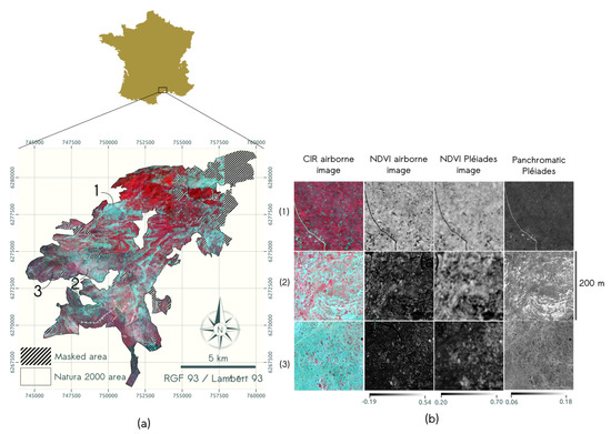
Figure 1.
(a) Study area with color infrared (CIR) airborne image and (b) examples of vegetation structures with CIR airborne image, NDVI airborne and Pléiades images, and Pléiades panchromatic image with (1) dense cover of low ligneous (LL) (Quercus coccifera); two structure types of highly mix of herbs (H) and LL with (2) early stage of encroachment by LL dominated by Quercus coccifera and (3) LL dominated by Juniperus oxycedrus. Radiometric dynamic is indicated by the greyscales for NDVI images and Pléiades panchromatic band.
Table 2.
List of the habitats of community interest that are present in Montagne de la Moure et Causse d’Aumelas site [47].
Image processing was restricted to the spatial extent defined by the Natura 2000 administrative boundaries, and anthropized surfaces, including built and agricultural surfaces, were excluded. In the context of textural analysis, the exclusion of agricultural surfaces is particularly important for vegetation showing periodic patterns, such as vineyards, olive and pine plantations. Clouds included in the Pléiades images were also masked. Total masked areas represent about 6% of the Natura 2000 site (9349 ha) and were delineated manually.
3. Methods
3.1. Characterization of Landscape Structure
3.1.1. Landscape Structure from Discrete Representation
The computation of landscape metrics is based on a discrete vegetation map. The following subsections describe the method used to produce the discrete vegetation map, and the type of landscape metrics computed from this vegetation map.
Vegetation Mapping
The vegetation map was produced from an object-based image analysis (OBIA) performed on the CIR airborne image. This OBIA aims at identifying four strata of interest corresponding to bare soil (BS), herbs (H), low ligneous (LL), i.e., shrubs or small trees, and high ligneous (HL). Here, the vegetation map derived from the airborne image was used as a reference, and the landscape metrics derived from this map were assumed to be stable between the airborne acquisition and the satellite acquisition one year later. The implementation of the vegetation map is detailed in Appendix A.
Computation of Landscape Structure Metrics
A variety of landscape metrics can be computed from the individual strata of the vegetation map. Although each landscape metric expresses a specific structural component, these metrics proved to be strongly redundant and intercorrelated [29,33,48,49]. Lang et al. [44] identified a set of metrics which could be accurately estimated from textural and radiometric indices. Here, we focused on two of these metrics, the percentage of landscape (PLAND), and the landscape shape index (LSI). PLAND provides information about the landscape composition, i.e., the proportion of each stratum in a given spatial unit. LSI provides information about the spatial configuration of each stratum. It is the ratio between the sum of the patches’ edges of a stratum and the minimum total edge possible, i.e., if all patches are aggregated into a single square patch. The minimum value is 1 if there is only one single square patch, and LSI increases when the number of patches increase or their shape diverges from a square and the length of the edges increase [50]. It can be interpreted as a measure of landscape disaggregation.
The two landscape metrics were computed for each stratum BS, H, LL and HL with FRAGSTATS 4.2.1 Software [50]. Two grouped strata were also computed: the ground (G) stratum, which corresponds to the combination of BS and H, and the ligneous (L) stratum, which corresponds to the combination of LL and HL. The landscape metrics were computed for a given window size across the landscape. Window boundaries were not counted as edges and metrics were computed with the eight neighbors rule within each window. The window size is mainly constrained by the information derived from the continuous representation and is defined in the next section.
3.1.2. Landscape Structure From Continuous Representation
The two textural indices were computed using the FOTO method. They provide information about the configuration of the vegetation [51,52,53,54]. The radiometric index corresponds to the NDVI and provide information about the proportion of individual vertical strata (BS, H, LL, HL), and the grouped strata (G and L). Combined, textural and radiometric indices provide complementary information about the composition and the configuration of each stratum [44].
The FOTO method produces textural gradients derived from frequency analysis of a single-band image. First, the image is divided into windows of homogeneous size. The window size is defined with respect to the type of landscape structure under study and the image spatial resolution: window size should be large enough to include several repetitions of the patterns of interest. Lang et al. [44] concluded that a window size of about 100 m was appropriate for Mediterranean landscapes as this size allows the method to capture canopy texture, individual trees and shrubs, as well as clumps of ligneous. Following the conclusions of Lang et al. [44], a window size of 108 m was chosen here. Second, a 2D Fourier transform is applied on each window, in order to produce a periodogram reflecting the share of variance accounted for by a given spatial frequency f, and traveling in a direction . The information is then averaged over all directions to produce a simplified 1D R-spectrum [55]. This directional averaging would be a strong limitation if the patterns of interest were expected to show anisotropic behavior, but this is not the case for our study site [44]. A Principal Component Analysis (PCA) is then applied on the R-spectra in order to extract the main components contributing to the frequency domain and reduce its dimensionality. Similarly to [44], only the two first components of the PCA (PC1 and PC2) were used to define indices related to coarseness texture attributes and to characterize vegetation structure.
Lang et al. [44] showed that the principal components produced by the FOTO method contained relevant information for the identification of a vegetation fragmentation textural gradient (VFTG), which is particularly important for the description for the vegetation structure in Mediterranean landscapes. This VFTG corresponds to a linear combination of the two first FOTO components PC1 and PC2. It is then possible to transpose this gradient along a single axis by applying a rotation of the 2D plane defined by PC1 and PC2. Lang et al. [44] linked the textural gradient orthogonal to the VFTG (hereafter TG-2) to the dominance of very fine texture produced by the canopy grain when applying FOTO on airborne images. Here, we aim at understanding if the VFTG can also be obtained from different types of satellite data when applying FOTO analysis, and if it is the case, which type of information corresponds to TG-2.
The radiometric index corresponding to the mean NDVI computed for each window enhances the capacity to discriminate structure among vegetation types when combined with textural information. Indeed, windows corresponding to different vegetation structures with opposite radiometric information (e.g., a matrix of herbaceous with shrubs vs. a matrix of shrubs with herbaceous gaps) may show similar textural attributes, leading to poor discrimination ability from textural indices only. Finally, the combination of VFTG, TG-2 and mean NDVI is a relevant set of indices for the characterization of vegetation structure.
3.2. Comparison of Vegetation Structure Among Data Sources
Four sets of indices were computed from the different datasets:
- ANDVI: both textural and radiometric indices were obtained from NDVI computed from airborne images (0.5 m spatial resolution);
- PPAN: textural indices were obtained from the P band of Pléiades imagery (0.5 m), while the radiometric index was obtained from the NDVI computed from the MS bands of Pléiades imagery (2 m);
- PNDVI: both textural and radiometric indices were obtained from the NDVI computed from the MS bands of Pléiades imagery (2 m);
- PNDVIFUS: textural indices were obtained from the NDVI computed from the panMS bands of Pléiades imagery (0.5 m), while the radiometric index was computed from the NDVI computed from the MS bands of Pléiades imagery (2 m).
Lang et al. [44] showed that regression models could be adjusted with textural and radiometric information obtained from ANDVI in order to estimate various landscape structure metrics. Here, we first aimed at testing the possibility to estimate landscape structure metrics from satellite images using the same methodology. Therefore, we compared the performance of regression models derived from airborne and spaceborne data for the estimation of PLAND and LSI (See Figure 2a). Secondly, we aimed at understanding the contribution of spatial resolution, radiometric information and pansharpenning products on the characterization of landscape structure: differences in mean NDVI values were studied (Figure 2b), then, the effect of spatial resolution was investigated by comparing ANDVI with PNDVI and the effect of radiometry was studied by comparing ANDVI with PPAN (Figure 2c). The effect of fusion was studied by comparing PNDVI with PNDVIFUS. ANDVI was not compared with PNDVIFUS, as our objective is to specifically understand the influence of pansharpening on textural gradients and landscape metrics estimation. Finally, we produced a RGB color composition from the three indices, VFTG, TG-2 and mean NDVI to map vegetation structure for each dataset and we compared the spatial dynamic of the vegetation structure (Figure 2c). A summary of the main acronyms used in the study is available in Table 3.
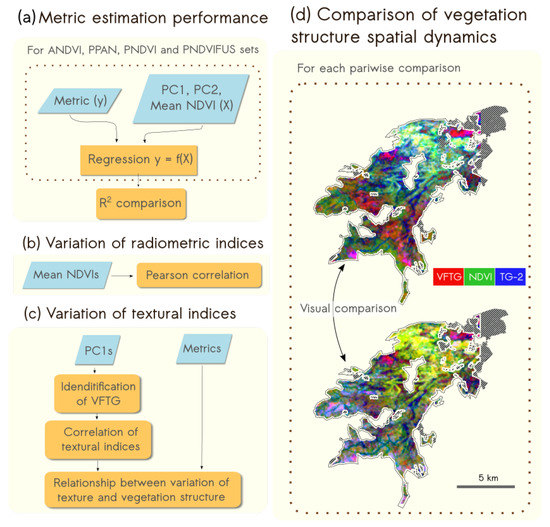
Figure 2.
Representation of the methodological framework used to study the influence of radiometry, spatial resolution and fusion on the characterization of vegetation structure with combined textural and radiometric indices with (a) the comparison of the estimation of landscape metric; the variation of (b) radiometric and (c) textural indices and (d) the comparison of the spatial representation of the vegetation structure with RGB maps representation.
Table 3.
List of the acronyms used in the study.
3.2.1. Estimation of Landscape Structure Metrics
RBF-SVM regression models [56] were adjusted from the principal components and the mean NDVI of ANDVI, PNDVI, PPAN and PNDVIFUS in order to estimate PLAND and LSI.
The dataset was randomly split into two different sets: a training set corresponding to 10% of the windows included in the study site (about 650 windows) and a validation set including the remaining windows. The optimization of C and was performed using an exhaustive grid search combined with a 5-fold cross validation, with values ranging from to for each parameter. The regression models were then applied on the validation dataset and the coefficient of determination between the landscape metrics derived from the discrete approach and the landscape metrics estimated from the continuous approach was used to estimate the performance of the regression. The training/validation process was repeated 30 times with different training/validation samples in order to test the sensitivity of the models to the training dataset.
3.2.2. Comparison of Radiometric Indices
The absolute value of the radiometric indices derived from Pléiades and airborne images are expected to differ since Pléiades images were expressed in top of atmosphere reflectance while airborne images were preprocessed and delivered as an orthorectified mosaic with a radiometric equalization performed among pictures. Therefore, we focused on a relative comparison and computed the Pearson correlation coefficient (PCC) between mean NDVI derived from airborne and spaceborne images.
3.2.3. Comparison of Textural Indices
Identification of the Vegetation Fragmentation Textural Gradient from Different Data Sources
As explained in Section 3.1.2, the VFTG is obtained after applying a rotation of 2D plane defined by PC1 and PC2 produced by FOTO when applied on airborne images. Our goal was to evidence if a textural gradient equivalent to the VFTG can be produced by FOTO when applied on satellite images. Our hypothesis was that such VFTG derived from satellite images should be correlated with the VFTG derived from airborne images, but that the rotation to be applied on the PC1-PC2 plane may vary with data source. Therefore, we needed to identify the rotation maximizing our ability to compare information among data sources.
We first identified the rotation angle needed to produce the VFTG from the airborne images. Next, we applied a rotation angle varying between 0° and 170° to the PC1 and the PC2 of the different satellite datasets. Finally, we selected the rotation angle maximizing the correlation between the rotated PC1 of:
- PPAN and the VFTG derived from airborne images;
- PNDVI and the VFTG derived from airborne images;
- PNDVIFUS and the VFTG derived from PNDVI.
Once the optimal rotation angle was found, the correlation among data sources was computed for VFTG and its orthogonal gradient TG-2.
Relationship between Textural Gradients and Vegetation Structure
After VFTG and TG-2 were defined for each dataset, we investigated the information contained in these textural gradients by relating the resulting 2D plane with vegetation structure. Our goal was to study the influence of spatial resolution and radiometric information on the relationship between the 2D plane and the vegetation structure. Our hypothesis was that changes in strata contrast occurring when using different radiometric information or spatial resolution result in changes in the dominant pattern enhanced by FOTO. To verify this hypothesis, we converted the position of each window in the 2D plane from Cartesian coordinate system to polar coordinate system. Such conversion allowed access to the dominant pattern enhanced by the 2D plane.
In the polar coordinate system, the radial distance r refers to the homogeneity of patterns present in a windows while the angle corresponds to most discriminatory pattern. Windows with low r values, i.e., windows located around the origin of VFTG / TG-2 plane, were expected to display a mix of patterns (textural heterogeneity), with one pattern slightly more discriminating than the others. On the contrary, windows with high r values were expected to display one strongly discriminating pattern (textural homogeneity), with the angle indicating its coarseness property.
Therefore, we focused on the identification in divergences in positions between data sources, and we investigated the potential relationship between specific vegetation structures described by PLAND and LSI and these changes in angular position. We arbitrarily defined the reference angle corresponding to in order to associate windows discriminated by coarse patterns to low angular values, and windows discriminated by fine patterns with high angular values.
3.2.4. Spatial Dynamics of Vegetation Structure
Finally, we produced a RGB color composition from the three indices, VFTG, TG-2 and mean NDVI. Based on these maps, we focused on five types of vegetation structure and compared the capacity to discriminate these types based on visual interpretation for each data source (Figure 2). These vegetation types correspond to:
4. Results
4.1. Classification of Vegetation Strata
Classification of the four strata resulted in an overall accuracy of 95% and a Kappa Coefficient of 0.93. All strata were accurately identified, with user and producer accuracies higher than 0.90 (Table 4). Minor confusions were observed between ligneous classes and between BS and H strata.
Table 4.
Confusion matrix of the vegetation map (BS: bare soil, H: herbs, LL: low ligneous, HL: High ligneous). Well classified regions appear in bold.
4.2. Estimation of Landscape Metrics
We aimed at testing the possibility to estimate landscape structure metrics from the proposed combination of textural and radiometric indices. Figure 3 summarizes the performance of the regression models for the estimation of PLAND (proportion of the strata) and LSI (disaggregation of the strata) from the continuous approach. Performance obtained for the estimation of PLAND was similar among data sources, with high coefficients of determination () for HL, G, L and for LL and H, and poor performance for the BS stratum ().
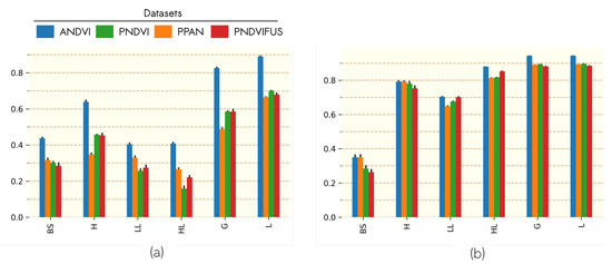
Figure 3.
Mean of coefficients of determination over 30 iterations of regression models predicting LSI (a) and PLAND (b) for each stratum and combination of strata with indices computed from different band. Error bars represent the standard deviation of coefficients of determination over the 30 iterations.
Performance obtained for the estimation of LSI did not show the same consistency among data sources as for PLAND. Better performance was systematically obtained for the estimation of metrics derived from ANDVI. Using NDVI information (PNDVI and PNDVIFUS) instead of panchromatic channel (PPAN) for FOTO analysis led to slightly improved estimation of LSI for herbs strata (H and G), but the performance among satellite data sources were similar when predicting other strata. No differences were evidenced when considering the effect of fusion (PNDVI vs. PNDVIFUS).
4.3. Comparison of Radiometric Indices
The differences between mean NDVI values of airborne images and Pléiades imagery are illustrated in Figure 4. Mean NDVI computed from Pléiades image ranged from 0.2 to 0.7 while mean NDVI values of computed from airborne images ranged from −0.19 to 0.55. Yet, a strong correlation in the mean NDVI of the two data sources was observed (). The mean NDVI computed from airborne images showed systematic underestimation compared to the mean NDVI computed from Pléiades images, which can be explained either by the different radiometric units corresponding to each type of image or by the difference in acquisition date. A comparison of Pléiades image and SPOT image taken at the end of June similarly to airborne images is presented in Appendix B. It must be noted that the vegetation state was stable between June and September, providing evidence that the variation observed (Figure 4) was mainly due to radiometric differences.
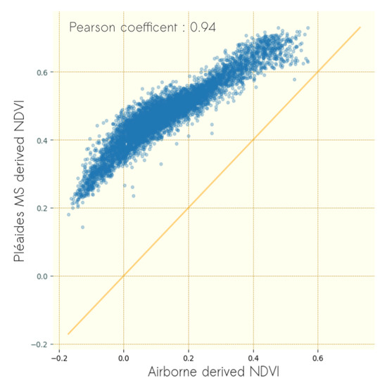
Figure 4.
Scatterplot of mean NDVI values of windows computed for 0.5 m resolution airborne imagery and 2 m resolution Pléiades imagery.
4.4. Comparison of Textural Indices
4.4.1. Identification of a Textural Index Corresponding to Vegetation Fragmentation
The first step was to identify the necessary orthogonal rotation angle to be applied on the PC1-PC2 plane computed from the airborne images in order to retrieve a textural gradient corresponding to vegetation fragmentation. The VFTG was obtained when applying a rotation of 30°. This VFTG corresponds to a gradient between low frequencies (coarse patterns) and high frequencies (fine patterns) (Figure A2, in the Appendix C).
Figure 5 illustrates the distribution of LSI and PLAND metrics for the G stratum (Figure 5a,c) and the L stratum (Figure 5b,d) in 2D space defined by VFTG and Mean NDVI. It illustrates the relationship between VFTG and LSI. Low VFTG values corresponded to low LSI and conversely, high VFTG values corresponded to high LSI. The mean NDVI was related to the dominant stratum. Low NDVI values corresponded to high percentage of BS (Figure 5a) and conversely, high NDVI values corresponded to high percentage of L (Figure 5b). The combination of VFTG with the mean NDVI revealed a continuous gradient of LSI for both G and L strata (Figure 5c,d, respectively), but for different ranges of NDVI. Similar relationships were found for individual strata and are presented in Figure A3a in the Appendix D.
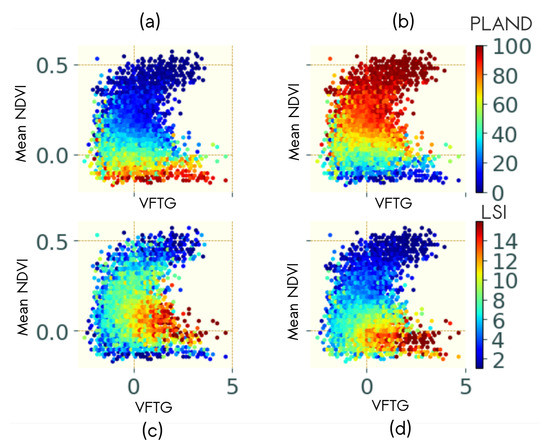
Figure 5.
PLAND (a,b) and LSI (c,d) distribution for (a,c) the grouped bare soil and herbs strata and (b,d) the grouped low and high ligneous strata on the 2D plane defined by the VFTG and mean NDVI computed on airborne images.
TG-2 was driven by very high frequencies (very fine texture) (Figure A2, in the Appendix C), and the relationship between Mean NDVI and TG-2 with LSI and PLAND was more difficult to interpret, especially for low TG-2 values. High TG-2 values were related to the dominance of HL cover for high mean NDVI and to high LSI values for low mean NDVI values (Figure A3b).
The second step was to identify the rotation maximizing our ability to compare information among data sources. Figure 6 shows the correlations between the VFTG obtained with airborne images and the first axis of the 2D plane after rotation of PC1 and PC2 derived from PNDVI and PPAN (Figure 6a,b). It also shows the correlations between the VFTG obtained with PNDVI and the first axis of the 2D plane after rotation of PC1 and PC2 derived from PNDVIFUS (Figure 6c).
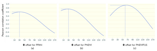
Figure 6.
Influence of loadings rotation on correlation of PC1 derived from (a) ANDVI with and PPAN with (b) ANDVI () and PNDVI with and (c) PNDVI () and PNDVIFUS with . The best correlation values are indicated in blue dotted lines.
The maximum correlation between VFTG derived from airborne data and the textural gradient computed from PNDVI and PPAN was obtained for a rotation of 30°, which corresponds to the rotation applied on ANDVI. The strong correlation between ANDVI and PNDVI () suggests that the VFTG derived from airborne images can also be captured from satellite data even with a decrease in spatial resolution from 0.5 m to 2 m. The moderate correlation between ANDVI and PPAN () suggests that the vegetation structure corresponding to VFTG can be partly captured when performing textural analysis on the panchromatic channel.
The maximum correlation between VFTG derived from PNDVI and the textural gradient computed from PNDVIFUS was obtained for a rotation angle of 60° (Figure 6c). The very strong correlation between the textural gradient corresponding to VFTG computed from PNDVI and the textural gradient computed from PNDVIFUS () suggests that both data sources share identical information, with strong correlation with the VFTG computed from airborne data.
Details on the correlations between the textural gradients VFTG computed from the different data sources and for the optimal rotation are illustrated in Figure 7. Pairwise comparisons illustrate the moderate to strong correlations among VFTG from different data sources identified in Figure 6.
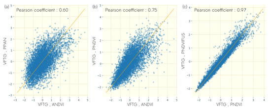
Figure 7.
Scatterplots of VFTG scores computed on (a) NDVI of airborne imagery (ANDVI) and panchromatic band of Pléiades imagery (PPAN) (b) ANDVI and NDVI of Pléiades imagery (PNDVI), (c) (PNDVI) and fusion derived NDVI of Pléiades imagery.
4.4.2. Correlation of TG-2 among Data Sources
The correlation between TG-2 computed from different data sources and for the optimal rotation is illustrated in Figure 8. It highlights the differences among datasets for TG-2.PCC TG-2 computed from ANDVI and from PPAN did not show correlation (, Figure 8a), suggesting that the very fine texture evidenced with TG-2 was related to different vegetation structure when computed from different radiometric information.
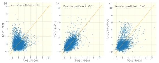
Figure 8.
Scatterplots of TG-2 scores computed on (a) NDVI of airborne imagery (ANDVI) and panchromatic band of Pléiades imagery (PPAN) (b) ANDVI and NDVI of Pléiades imagery (PNDVI), (c) (PNDVI) and fusion derived NDVI of Pléiades imagery.
TG-2 computed from ANDVI and from PNDVI showed moderate correlation (, Figure 8b), suggesting that the textural information contained in the two first textural gradients derived from FOTO was related to relatively similar vegetation structure with the decrease in spatial resolution.
The comparison of TG-2 computed from PNDVI and from PNDVIFUS shows weak correlation (, Figure 8c), suggesting that while the first textural gradient corresponding to vegetation fragmentation was preserved during fusion, the orthogonal textural gradient was related to different vegetation structures.
The correlations between the 2D plane defined by the VFTG and the TG-2 and spatial frequencies are presented in Figure A2 in the Appendix C. It illustrates that gradients of all data sources after rotation expressed a contrast between the same relative range of frequencies, i.e., between the same coarseness attributes, while there were not all correlated. It means for instance that a window with high score in TG-2 displayed a very fine texture for all data sources. However, it did not imply that this very fine texture was related to the same vegetation structure.
4.4.3. Linking Textural Gradients to Vegetation Structure
4.4.3.1. Influence of Spatial Resolution
The influence of the spatial resolution on the dominant pattern evidenced by the textural indices is illustrated in Figure 9. The polar angle corresponding to the position of each window in polar coordinates showed relatively good agreement between ANDVI and PNDVI (Figure 9a). Windows corresponding to low angular values in ANDVI and high angular values in PNDVI, and vice versa (identified as (1) and (2) in Figure 9a respectively), corresponded to windows showing particular sensitivity to the degradation of the spatial resolution. Indeed, very fine patterns were more difficult to detect in PNDVI, favoring the distinction of relatively finer patterns or coarser patterns (zones (1) and (2) Figure 9, respectively). Changes in coarseness attributes did not seem related to specific vegetation structure and thus the texture-vegetation relationship remained stable with differences in spatial resolution.
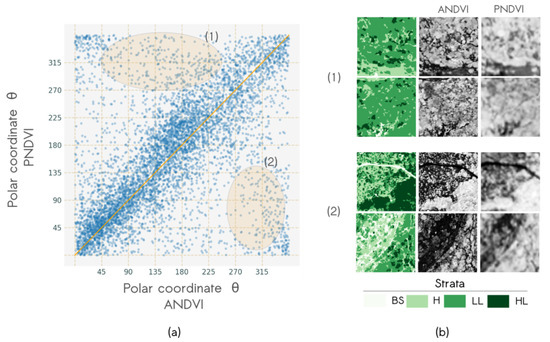
Figure 9.
Co-variation of textural gradients derived from airborne imagery NDVI and Pléiades NDVI band: (a) Scatterplot of angular coordinates with two types of angular variations highlighted in orange: (1) from [45°, 225°] to [270°, 360°], (2) from [270°, 360°] to [0°, 135°], and (b) typical windows of each variation type.
4.4.3.2. Influence of Pansharpenning
The influence of the pansharpenning on the dominant pattern evidenced by the textural indices is illustrated in Figure 10. Pansharpening resulted in much stronger changes in angular values, especially for high values. First, the comparison of obtained from PNDVI and PNDVIFUS (Figure 10a) shows that low angular values ( lower than 180°) were highly related. It indicates that when the most discriminatory pattern was a coarse pattern ( lower than 180°) in window characterized with PNDVI, the most discriminatory pattern was also a coarse pattern with PNDVIFUS. Nevertheless, the slope lower than 1 for values lower than 140° indicated that PNDVIFUS was less sensitive to very coarse patterns than PNDVI. Angular values higher than 180° were very different among data sources and two variation types were observed. One corresponding to windows that had higher values in PNDVIFUS and another where windows had lower values in PNDVI (identified as (1) and (2) Figure 10a, respectively). Plotting the distribution of landscape metrics of windows (1) and (2) against the distribution of all windows showed that windows (1) and (2) had a high percentage of HL and LL, respectively (Figure 10b). Fusion algorithm allowed for the emergence of very fine texture for HL stratum but not for LL stratum as illustrated in representative windows of zone 1 and 2 in Figure 10c. These results explained the high correlation between the two VFTG and the relatively low correlation of the TG-2.
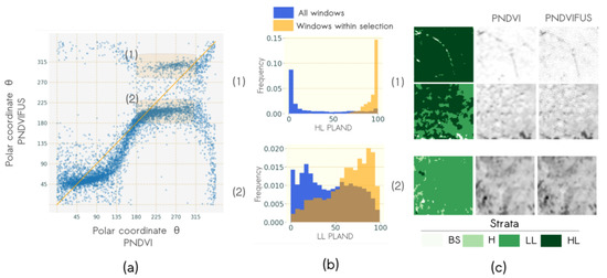
Figure 10.
Co-variation of textural gradients derived from NDVI of Pléiades before and after pansharpenning and: (a) Scatterplot of angular coordinates with two types of angular variations highlighted in orange: (1) from [180°, 315°] to [280°, 330°], (2) from [180°, 315°] to [200°, 250°]; (b) histograms of characteristic vegetation structure of each angular variation type, metric distribution is plotted in blue when considering all windows and in orange when considering only windows within the variation type angular range values, and (c) typical windows of each variation type.
4.4.3.3. Influence of Radiometry
The influence of the radiometric information on the dominant pattern evidenced by the textural indices is illustrated in Figure 11. It corresponds to the variations of angular values between ANDVI and PPAN. Figure 11a. shows that there were many differences in the most discriminatory patterns within windows of the two data source. Four types of variations were identified (zones 1, 2, 3 and 4 in Figure 11a, respectively).
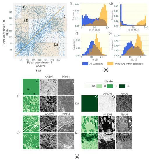
Figure 11.
Co-variation of texture gradients derived from airborne imagery NDVI and Pléiades panchromatic band: (a) Scatterplot of angular coordinates with four types of angular variations highlighted in orange: (1) from [45°, 225°] to [270°, 360°], (2) from [270°, 360°] to [180°, 270°], (3) from [135°, 315°] to [0°, 90°] and (4) from [0°, 90°] to [135° to 270°]; (b) typical windows of each variation type and (c) histograms of characteristic vegetation structure of each angular variation type, metric distribution is plotted in blue when considering all windows and in orange when considering only windows within the variation type angular range values.
The distribution of landscape metrics LSI and PLAND corresponding to windows within these zones was compared to the general distribution corresponding to all windows and showed that zone 1 and zone 2 corresponded to windows with a high percentage of LL and HL, respectively (Figure 11b). These vegetation structures were characterized by different coarseness attributes in ANDVI and PPAN. On the one hand, variations in zone 1 were explained by the very fine intra LL texture, visible only in PPAN (see (1) in Figure 11c). On the other hand, variations in zone 2 were explained by the presence of shadows in the HL canopy visible only in PPAN that produced a coarser texture than the texture of HL canopy in ANDVI (see (2) in Figure 11c).
Zone 3 and zone 4 were characterized by a higher disaggregation of H and LL, respectively, than the overall disaggregation (see (3) and (4) Figure 11b). These variations could be explained by the lower contrast between L and G strata in PPAN. Thus, inter G/L patterns were less discriminated during the frequency analysis, favoring the distinction of other patterns. In the case of zone 3, fine patterns due to the G/L contrast in ANDVI decreased for the benefit of very coarse patterns produced by a higher contrast of BS and vegetation in PPAN (see (3) in Figure 11c). Conversely, very coarse patterns due to the G/L contrast in ANDVI decreased for the benefit of a finer texture produced by small shrubs or intra H texture (see (4) in Figure 11c).
These results showed that changes in coarseness attributes were then related to a specific vegetation structure when considering data sources of different radiometry. The changes of vegetation contrast in windows characterized by heterogeneous structure (i.e., high LSI) explained the variability observed between the VFTG of the two data sources (Figure 7a). In addition, the difference of the canopy grain texture of LL and HL for the two data sources explained the absence of the correlation observed for the TG-2 (Figure 8b). As a consequence, the interpretation of these gradients in terms of vegetation structure was different when derived from different radiometric information.
Finally, the VFTG initially derived from textural analysis of the airborne images could also be identified in satellite data sources. Yet, in case of windows containing heterogeneous patterns, high variability in VFTG were observed when using different radiometric information (PPAN) because of changes in vegetation contrast. The TG-2 corresponding to canopy grain texture of HL derived from textural analysis of the airborne images could also be identified from NDVI data sources (PNDVI and PNDVIFUS). However, the TG-2 were related to canopy grain of LL for PPAN data source.
4.5. Spatial Dynamics of Vegetation Structure
A RGB color composition from the three indices, VFTG, TG-2 and mean NDVI was produced for each dataset. It allowed comparing the spatial representation of the vegetation structure when using data sources of different spatial resolutions and radiometric information. Figure 12 shows the color composite including VFTG, mean NDVI and TG-2: the intensity of the red channel corresponds to the degree of disaggregation (VFTG); while the intensity of the green channel corresponds to the proportion of L characterized by higher NDVI, and the intensity of the blue channel corresponds to the presence of very fine textural content. This blue channel, could be linked to different “canopy” grains depending on the data source as explained in Section 4.4.3.2.
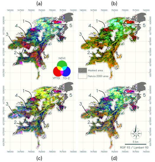
Figure 12.
Maps of combined textural and radiometric indices of (a) ANDVI, (b) PNDVIFUS, (c) PPAN and (d) PNDVI using a RGB color composition (with R = VFTG, G = mean NDVI, B = TG-2). Main vegetation structure types are located on the maps by arrows with two structure types of highly mix of herbs and low ligneous with (1) early stage of encroachment of herbs by low ligneous (Quercus coccifera); (2) herbs and low ligneous (Juniperus oxycedrus); (3) dense cover of low ligneous (Quercus coccifera); (4) dry grassland and (5) forest.
The RGB map produced with ANDVI highlights the contrast among vegetation structures (1 to 5 in Figure 12a) as follows:
- mosaics of disaggregated LL and H are displayed in orange, red and magenta, depending on the relative proportion of each stratum (structure types 1 and 2);
- continuous covers of LL are displayed in green (structure type 3);
- continuous covers of H are displayed in dark blue (structure type 4);
- dense continuous HL are displayed in yellow, bright green or cyan (structure type 5 in Figure 12).
The contribution of the spatial resolution was analyzed by comparing the RBG maps derived from ANDVI and PNDVI. The RGB map derived from PNDVI (Figure 12d) showed similar spatial patterns, associated with the same colors as the map derived from ANDVI, as suggested by the correlations between VFTG and TG-2 scores (Figure 7 and Figure 8). However, the distinction between continuous LL cover and disaggregated LL and H varied depending on the type of dominant LL species: highly disaggregated structures were accurately characterized for Juniperus oxycedrus while LL dominated by Quercus coccifera showed lower contrast in red tones (structure type 1 and 2, respectively, in Figure 12d)
The contribution of the radiometric information was analyzed by comparing the RBG maps derived from ANDVI and PPAN. The RGB map derived from PPAN (Figure 12c) also allowed identifying the main vegetation structure types. Though, they were not associated with the same colors as in ANDVI map, as suggested by the absence of correlation between TG-2 scores (Figure 8). Dense continuous HL shifted from bright green and cyan in ANDVI map to yellow in PPAN map. Conversely, continuous cover of LL shifted from green to magenta or blue-gray, due to very fine texture of LL visible only in PPAN. Similarly to PNDVI map, highly disaggregated structures for LL dominated Juniperus oxycedrus was better characterized than LL disaggregated structure of Quercus coccifera.
More details on the influence of radiometry on Quercus coccifera structure is detailed in Figure 13. It presents a transect in which a mosaic of LL and H were present for different combinations of PLAND and LSI values (Figure 13a,b). First, contrast between the two strata was higher for the NDVI band of airborne images than the P image of Pléiades (Figure 13d). Consequently, ANDVI RGB map showed shades of pink-red-orange in high disaggregated parts (2 to 5 in Figure 13) characterizing well the heterogeneity of vegetation structure. The contrast between parts 2 and 3 and between parts 3 and 4 was lower, and parts 4 and 5 showed no clear differences in colors in PPAN RGB map, leading to a lower characterization of LL-H heterogeneity. The emergence of LL very fine texture in PPAN was also visible in part 1 with LL displaying blue-gray versus green in ANDVI derived map.
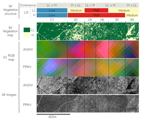
Figure 13.
Influence of the radiometric information for mapping vegetation structure on a transect of mixed LL (Quercus coccifera) and H strata containing a (a) gradient of vegetation structure in both terms of relative composition and configuration (LSI), derived from a (b) vegetation map. (c) RGB composite maps (with R = VFTG, G = NDVI, B = TG-2) and (d) the corresponding data source for textural analysis.
5. Discussion
5.1. Stability of Textural Contrast
The textural information produced from FOTO showed consistency in term of texture contrast when derived from airborne to satellite images with different radiometric information and spatial resolution. Rotation of original PCs of FOTO method always allowed retrieving the gradients VFTG and TG-2 expressing a contrast between the same coarseness attributes: very coarse against fine patterns for VFTG and the dominance of fine pattern for TG-2. The same rotation angles of 30° were found for ANDVI, PPAN and PNDVI, indicating that the decomposition of the spatial frequencies was stable among data sources with different radiometric information and spatial resolution. However, texture contrast evidenced by FOTO may differ for spatially distinct area as suggested in barbier and Couteron [57] and Bastin et al. [58]. For instance, texture contrasts expressed by principal components derived from the same airborne imagery on a subset area of the current study site were different and a different rotation angle of 60° was necessary to retrieve a gradient expressing the contrast between very coarse patterns and patterns [44]. Furthermore, the principal components computed from PNDVIFUS differed from those computed from the other data sources.
The optimization of the rotation angle based on a reference textural gradient proved to be efficient when the VFTG and TG-2 were not defined identically along the PCs of FOTO method, as it was the case for PNDVIFUS whose optimal rotation angle was 60°. It pleads towards the stability of FOTO textural gradients in terms of texture contrast over various landscapes. Indeed, FOTO PCs derived from different ecosystems with similar data (e.g., [53,54,57]) or with different data like digital elevation models [59], indicate that rotation would allow retrieving VFTG and TG-2 in terms of texture contrast.
The stability of texture gradient in coarseness contrast constitutes a first milestone for the monitoring of vegetation structure in complex heterogeneous landscapes. However, it does not mean that the spatial distribution of texture features is the same within the images but rather that it is the same globally. It also does not guarantee that VFTG and TG-2 obtained after rotation are similarly related to vegetation structure. This very point is discussed hereafter.
5.2. Implication of the Use of Spaceborne Data for Monitoring Vegetation Structure
This study confirms the potential of FOTO textural indices for providing relevant information about continuous change in landscape structure, when combined with the NDVI using airborne image. Here, the use of an object-based approach showed significantly improvement in classification accuracy as reported by other studies (e.g., Hamada et al. [60]). In particular, as compared to previous study [44], indices computed from airborne images led to a higher ability to estimate metrics when metrics were computed from vegetation map computed using an object-based approach. This reinforces the existence of the relationship between textural gradients and vegetation fragmentation using airborne images, in particular over large extents.
The ability of Pléiades images to characterize vegetation structure similarly to airborne images raised questions related to how spatial and radiometric information influence the characterization of landscape structure and its representation. We showed that spaceborne NDVI images of lower resolution than airborne images, and spaceborne panchromatic images allowed characterizing vegetation structure. However, NDVI information at 0.5 m spatial resolution was necessary to be able to encompass the whole heterogeneity of vegetation structure. All in all, taking advantage of both higher spatial resolution and NDVI led to a systematically better relation with LSI and PLAND metrics, for any stratum considered.
A more detailed comparison of textural indices showed that NDVI satellite image at 2 m provided relevant information on the vegetation structure that was similar to airborne derived NDVI. VFTG and TG-2 can be used and interpreted similarly for most of the structural heterogeneity measurements. High correlation among gradients () and the visual comparison of landscape representation evidenced that the relationship between texture gradients remained stable with lower NDVI spatial resolution. Very fine scale heterogeneity of the structure specific to Juniperus oxycedrus mixed with H was well characterized. However, 2 m spatial resolution was not precise enough to capture very fine scale heterogeneity of the structure specific to Quercus coccifera mixed with H. In that regards, NDVI information at 0.5 m spatial resolution is necessary to produce VFTG and TG-2 gathering the whole structural gradient.
Our attempts to overcome this limitation and to benefit from the spatial information of the panchromatic image using pan-sharpening method showed poor results. Only the textural characterization of forest canopy was enhanced by the data fusion, but it did not allow finer characterization of LL/H patterns. Johnson [61] demonstrated that the choice of the algorithm may dramatically influence the efficiency of the fusion when followed by NDVI computation. Preliminary tests (not shown here) on the choice of the pan-sharpening algorithm were realized and also showed poor results. Yet, only common algorithms available in the OTB were tested whereas the question deserves thorough investigations as 0.5 m spatial resolution is needed to catch whole structural gradient, including fine scale disaggregated structure related to early stage of encroachment by Quercus coccifera.
Regarding the influence of radiometry on vegetation structure monitoring, panchromatic and NDVI images showed similar potential for the delineation of management units. This is a crucial step towards improvement of management of protected areas and on biodiversity conservation [62]. Indeed, continuous indices derived from panchromatic and NDVI images allowed similar distinction of vegetation types as illustrated on the RGB maps. However, the differences in the contrast among vegetation strata changed the relationship between textural gradients and vegetation structure, and they brought out details on patterns related to different strata. Thus, panchromatic and NDVI information shows potential for distinct applications.
NDVI information should be preferred in application linked to landscape closure dynamics like habitat degradation caused by shrubs encroachment [25,63], fire propagation management [64] or changes in bird communities composition [14]. Indeed, ANDVI indices are better suited for the characterization of LL structure when mixed to both H and BS because of contrast between both strata that is far lower than either LL/BS or LL/H contrast, as shown in Figure 11 and Figure 13. Conversely, panchromatic derived information brings more details on BS/H patterns and may be more relevant in applications focusing on grazing management like the detection of over grazing [65,66].
Another main difference between ANDVI and PPAN indices is that their TG-2 were related to totally different vegetation structures. Canopy grain evidenced by the TG-2 was no longer associated with the forest canopy but to shrub canopy texture that was visible only with panchromatic information. If the potential of FOTO for tropical forest management is well-known (for e.g., [67,68,69]), its aptitude has not been demonstrated for the monitoring of the development stage of continuous covers of shrubs. Textural information derived from panchromatic images shows potential in that matter and it may open up promising opportunities for the monitoring of vegetation flammability through biomass estimation which is a main issue for fire risk management in Mediterranean areas [70].
The combination of the two textural gradients VFTG and TG-2 with the mean NDVI proved to be a relevant set of indicators of vegetation structure derived from satellite images. Most of the computation process is unsupervised, and they provide information on four vertical strata in terms of composition and configuration. In addition, mapping these indicators provided synoptic information which could be interpreted in terms of vegetation structure. Thus, they show strong potential for habitat mapping and habitat condition assessment. Our framework shows strong potential for the monitoring biodiversity and the improvement of natural habitat mapping. The approach could serve directly to the French terrestrial vegetation mapping initiative that needs to be implemented at a country level (known as CarHAB). These indicators can also contribute to the monitoring of bird species that are very sensitive to landscape closure and related vegetation structural changes in heterogeneous mosaics (Lang et al. in prep). In addition, the integration of the VFTG and TG-2 shows potential to contribute to the long-term assessment of conservation programs as FOTO method was initially designed for historical aerial imagery [52].
5.3. Further Directions towards Operational Monitoring
The influence of several factors on the proposed indices still needs to be assessed to capture critical scales and dimensions of biodiversity, and to warrant their generalizability. For instance, the scene illumination is a well-known factor that influences the textural characterization of forest canopy [51,57]. Hence, it is likely that the relationship between TG-2 and canopy texture of HL or LL strata varies with geometry acquisition. Indeed, the main difference between NDVI and panchromatic data sources was related to the TG-2 and it was due to the appearance in the panchromatic image of very fine texture of LL in one hand and to the coarser texture of HL canopy in the other hand. This could be explained by the presence of shadows that were far less present in aerial images. Thus, influence of scene illumination should deserve more investigation. Yet, it does not deny the relevance of the proposed indices to be used as indicators of vegetation structure: firstly because illumination effects can be mitigated to some extent [57] and secondly because its influence on fragmentation pattern, i.e., VFTG, was not observed in this study.
Using different radiometry data sources highlighted that changes in vegetation contrast influence the relationship between textural gradient and vegetation structure. It is likely that phenology of the vegetation also influences frequency analysis, especially for NDVI data sources. In this study, we considered that the vegetation state was stable between the two dates of acquisition of the airborne images (end of June) and the Pléiades (beginning of September). However, an offset between NDVI values of airborne and spaceborne images was observed, suggesting that vegetation state varied. Thus, we compared NDVI values of Pléiades with another data source: a SPOT image acquired at the same period (end of June) as the airborne images. We concluded that the variations observed between airborne and Pléiades images was mostly due to the differences in radiometric unit. Nonetheless, the contribution of phenology to the characterization of vegetation structure is crucial and need to be assessed as acquisition in early spring may result in a diminution of H/L contrast while increasing contrast of LL/HL.
Further research is still needed to assess the potential of combining textural gradients obtained at different seasons for enhanced characterization of vegetation strata. Similarly, a promising lead for further implementation is to consider the combination of NDVI and panchromatic information for a richer continuous characterization of vegetation structure by using VFTG and TG-2 of both data source, which proved to bring complementary information. One solution may consist in running a second “global” PCA with the four gradients of FOTO to provide new synoptic indicators taking advantage of information present in both data sources. Bugnicourt et al. [59] illustrated it for regional land forms and landscape mapping. Nevertheless, the link between these indices and vegetation structure would require to be reassessed.
6. Conclusions
The use of VHSR spaceborne data is crucial for monitoring biodiversity because it allows getting information over large areas, potentially several times a year as opposed to airborne images. Results proved the ability of Pléiades satellite imagery to provide relevant indicators of the structure of various vertical vegetation strata. The tests performed led to learn about the influence of downscaling the spatial resolution to 2 m. In particular, using panchromatic radiometric information on the final characterization and representation of the landscape structure was proven useful. High resolution satellite data proved to be valuable for vegetation structure monitoring even if it appeared that NDVI information at 0.5 m spatial resolution is still needed to produce indices that could gather the whole structural gradient in very heterogeneous landscapes. However, the upcoming arrival of the new Pléiades Neo constellation with 0.30 m of spatial resolution will soon allow benefiting from images with similar technical characteristics to airborne images. It may enable to test the present framework to contribute to the management of Mediterranean vegetation at regional scale. The use of high resolution data provided a valuable source for primary observation in relation to vegetation structure to address the current conservation needs, in particular provides an operational method to assess habitat conditions while supporting mapping to inform conservation planning.
Author Contributions
Conceptualization, M.L., S.A., S.L., N.B. and J.-B.F.; Formal analysis, M.L. and J.-B.F.; Methodology, M.L. and J.-B.F.; Supervision, S.A., S.L., N.B. and J.-B.F.; Visualization, M.L.; Writing—original draft, M.L.; Writing—review & editing, M.L., S.A., S.L., N.B. and J.-B.F.
Funding
This research was funded by French National Research Agency grand number ANR-10-EQPX-20 in the framework of GEOSYD, by French the National Research Institute of Science and technology for Environment and Agriculture (IRSTEA) the APC was funded by the French Space Study Center (CNES, TOSCA 2018). The authors also thank the French “Ministère de la Transition Ecologique et Solidaire (MTES)” for financial support.
Conflicts of Interest
The authors declare no conflict of interest.
Appendix A. Vegetation Mapping
The implementation of the vegetation map was performed in three distinct steps. First, segmentation was performed with the Generic Region Merging segmentation algorithm [71] in order to delineate regions corresponding to homogeneous surfaces. The parametrization of this algorithm implemented in OTB was performed based on visual inspection of the results for different values of scale and homogeneity parameters. Scale and homogeneity parameters control the size and the shape complexity of the regions, respectively. The segmentation was judged as satisfying when regions corresponding to a selection of sub areas representative of the diversity of the vegetation structure observed in the image were properly delineated. i.e., small shrubs corresponding to a size of a limited number of pixels were delineated while the over-segmentation of forest or large patch of shrubs was avoided as far as possible. Finally, optimal values for scale and homogeneity were set to 15 and 0.5, respectively.
Next, a set of regions homogeneously distributed across the whole study site was selected and labeled for each of the four strata of interest: the site was divided into 16 ha windows and one region corresponding to each class was labeled when possible. We defined here low ligneous as ligneous comprised between 0.5 m and 2 m and ligneous above 2 m were defined as high ligneous. Hence, most of the low ligneous corresponded to shrubs but this designation also included young trees. Samples were taken by photo-interpretation and for the low ligneous stratum, we both digitized shrubs and small trees. We distinguished individual young trees from more advanced growth stages by their crown size and their visual aspect (i.e., their texture). This sampling resulted in 1661 regions, which distribution is detailed in Table A1.
Table A1.
Number of samples regions per vegetation stratum. BS: bare soil; H: herbs; LL: Low ligneous; HL: High ligneous.
Table A1.
Number of samples regions per vegetation stratum. BS: bare soil; H: herbs; LL: Low ligneous; HL: High ligneous.
| Vegetation Stratum | Number of Regions | Number of Pixels | Mean Number of Pixels Per Region |
|---|---|---|---|
| BS | 401 | 90 353 | 225 |
| H | 408 | 78 289 | 191 |
| LL | 433 | 73 645 | 170 |
| HL | 369 | 52533 | 142 |
Then, a set of features was computed from the radiometric information corresponding to each region: mean, standard deviation, 2nd and 98th quantile corresponding to each spectral band (green, red and infrared). Quantile statistics were preferred to minimum and maximum in order to avoid influence of outliers. These 12 region’ features where then used in a support vector machine (SVM) classification with a radial basis function (RBF) kernel [72]. The initial set of regions was randomly split into a training set and a validation set equally distributed (50% for each). The RBF-SVM classifiers require two free parameters to be optimized, C and . C is the cost parameter corresponding to the trade-off between penalization of wrongly classified samples and maximal margins between classes. is the inverse of the standard deviation of the RBF kernel, which is used as similarity measure between two points. It controls the trade-off between error due to bias and variance in the model. The strategy followed for this optimization is based on an exhaustive grid search strategy with a five-fold cross validation using the training set aiming at maximizing overall accuracy of the classifier. The space defined by C values ranging from to and values ranging from to 10 was explored. Then, the model was trained using the full training sample set with optimal values found in the previous step. The performance of the classification was assessed with the validation sample set using kappa coefficient, overall accuracy, user accuracy and producer accuracy for each vegetation stratum.
Appendix B. Influence of Phenology
We concluded in Section 4.3 that the offset of mean NDVI values observed between airborne and Pléiades imagery (Figure 4) could be explained either by the different radiometric units corresponding to each type of image, or by the difference in acquisition date. In this appendix, we discuss further the influence of phenology on the vegetation state as seen by a spaceborn sensor.
Most of the ligneous vegetation is evergreen vegetation in our study site. Evergreen ligneous only renew a fraction of their foliage (about 30%) yearly, since their leaves are photosynthetically active for several years [73]. In the case of Quercus ilex and Quercus coccifera, the two main ligneous species present in our study site, the leaves flush occurs in April/May and leaf shedding occurs in May-June-July [73,74,75]. As a consequence, most of the phenological variations occurred before the acquisition scene of airborne images. Therefore, we hypothesized that the state of vegetation was comparable between the end of June and the beginning of September.
To verify this hypothesis, we used a SPOT image acquired at the same period as the airborne images but for a different year. The SPOT image was acquired on the June 23 of 2016. The four multi-spectral bands correspond to the blue (455–525 nm), the green (530–590 nm), the red (625–695 nnm) and the near infra-red (760–890 nm), available at 6 m spatial resolution. First, the image was converted into top of atmosphere reflectance. Then, the mean NDVI of windows of 108 m size were computed. Finally, we analyzed the linear relationship between the mean NDVI of the SPOT image and the Pléiades images in Figure A1.

Figure A1.
Scatterplot of mean NDVI values of windows computed for 6 m resolution of SPOT imagery and 2 m resolution Pléiades imagery.
We evidenced a strong linear relationship between the NDVI of the two images (). A slope of 1.00 and an intercept of −0.06 were found, indicating a slight decrease of the mean NDVI value between the end of June and the beginning of September. These results support our hypothesis that the vegetation state is stable between these two periods and that the variation observed between airborne and Pléiades imagery were mostly due to the differences in radiometric units.
The SPOT images was acquired one year after the airborne images. If no strong inter annual variations of the climate were reported between these two years, an image taken at the same year would be necessary to strictly confirm this result.
Appendix C. Correlation between Frequencies and Textural Gradients

Figure A2.
Correlation between spatial frequencies (expressed in cycles.km) and Vegetation Fragmentation Gradient Texture (VFTG) and Canopy Grain Gradient Texture (TG-2) derived from (a) NDVI band of airborne imagery, (b) NDVI band of Pléiades imagery, (c) panchromatic band of Pléiades imagery and (d) fusion derived NDVI of Pléiades imagery; after optimal rotation of 30 original principal component 1 and 2 for (a–c) and 60° for (d).
Appendix D. Relationship between Textural and Radiometric Indices and Landscape Metrics

Figure A3.
PLAND and LSI distribution for bare soil (BS), herbs (H), low ligneous (LL), high ligneous (HL), on the 2D plane defined by (a) the VFTG and mean NDVI and (b) the TG-2 and the mean NDVI computed on airborne images.
References
- Atauri, J.A.; de Lucio, J.V. The role of landscape structure in species richness distribution of birds, amphibians, reptiles and lepidopterans in Mediterranean landscapes. Landsc. Ecol. 2001, 16, 147–159. [Google Scholar] [CrossRef]
- Lawley, V.; Lewis, M.; Clarke, K.; Ostendorf, B. Site-based and remote sensing methods for monitoring indicators of vegetation condition: An Australian review. Ecol. Indic. 2016, 60, 1273–1283. [Google Scholar] [CrossRef]
- Redon, M.; Bergès, L.; Cordonnier, T.; Luque, S. Effects of increasing landscape heterogeneity on local plant species richness: How much is enough? Landsc. Ecol. 2014, 29, 773–787. [Google Scholar] [CrossRef]
- Nagendra, H.; Lucas, R.; Honrado, J.P.; Jongman, R.H.; Tarantino, C.; Adamo, M.; Mairota, P. Remote sensing for conservation monitoring: Assessing protected areas, habitat extent, habitat condition, species diversity, and threats. Ecol. Indic. 2013, 33, 45–59. [Google Scholar] [CrossRef]
- Pereira, H.M.; Ferrier, S.; Walters, M.; Geller, G.N.; Jongman, R.H.G.; Scholes, R.J.; Bruford, M.W.; Brummitt, N.; Butchart, S.H.M.; Cardoso, A.C.; et al. Essential Biodiversity Variables. Science 2013, 339, 277–278. [Google Scholar] [CrossRef] [PubMed]
- Skidmore, A.K.; Pettorelli, N.; Coops, N.C.; Geller, G.N.; Hansen, M.; Lucas, R.; Mücher, C.A.; O’Connor, B.; Paganini, M.; Pereira, H.M.; et al. Environmental science: Agree on biodiversity metrics to track from space. Nature 2015, 523, 403–405. [Google Scholar] [CrossRef] [PubMed]
- Blondel, J.; Aronson, J. Biology and Wildlife of the Mediterranean Region; Oxford University Press: Oxford, UK, 1999. [Google Scholar]
- Myers, N.; Mittermeier, R.A.; Mittermeier, C.G.; Da Fonseca, G.A.; Kent, J. Biodiversity hotspots for conservation priorities. Nature 2000, 403, 853–858. [Google Scholar] [CrossRef] [PubMed]
- Medail, F.; Quezel, P. Hot-spots analysis for conservation of plant biodiversity in the Mediterranean Basin. Ann. Mo. Bot. Garden 1997, 84, 112–127. [Google Scholar] [CrossRef]
- Cowling, R.M.; Rundel, P.W.; Lamont, B.B.; Arroyo, M.K.; Arianoutsou, M. Plant diversity in Mediterranean-climate regions. Trends Ecol. Evol. 1996, 11, 362–366. [Google Scholar] [CrossRef]
- Thompson, J.N. The Geographic Mosaic of Coevolution; University of Chicago Press: Chicago, CA, USA, 2005. [Google Scholar]
- Blondel, J. The ‘design’of Mediterranean landscapes: A millennial story of humans and ecological systems during the historic period. Hum. Ecol. 2006, 34, 713–729. [Google Scholar] [CrossRef]
- Debussche, M.; Lepart, J.; Dervieux, A. Mediterranean landscape changes: Evidence from old postcards. Glob. Ecol. Biogeogr. 1999, 8, 3–15. [Google Scholar] [CrossRef]
- Sirami, C.; Nespoulous, A.; Cheylan, J.P.; Marty, P.; Hvenegaard, G.T.; Geniez, P.; Schatz, B.; Martin, J.L. Long-term anthropogenic and ecological dynamics of a Mediterranean landscape: Impacts on multiple taxa. Landsc. Urban Plan. 2010, 96, 214–223. [Google Scholar] [CrossRef]
- Shoshany, M. Satellite remote sensing of natural Mediterranean vegetation: A review within an ecological context. Prog. Phys. Geogr. 2000, 24, 153–178. [Google Scholar] [CrossRef]
- Lloret, F.; Calvo, E.; Pons, X.; Díaz-Delgado, R. Wildfires and landscape patterns in the Eastern Iberian Peninsula. Landsc. Ecol. 2002, 17, 745–759. [Google Scholar] [CrossRef]
- Moreira, F.; Viedma, O.; Arianoutsou, M.; Curt, T.; Koutsias, N.; Rigolot, E.; Barbati, A.; Corona, P.; Vaz, P.; Xanthopoulos, G.; et al. Landscape—Wildfire interactions in southern Europe: Implications for landscape management. J. Environ. Manag. 2011, 92, 2389–2402. [Google Scholar] [CrossRef]
- Brummitt, N.; Regan, E.C.; Weatherdon, L.V.; Martin, C.S.; Geijzendorffer, I.R.; Rocchini, D.; Gavish, Y.; Haase, P.; Marsh, C.J.; Schmeller, D.S. Taking stock of nature: Essential biodiversity variables explained. Biol. Conserv. 2017, 213, 252–255. [Google Scholar] [CrossRef]
- Feld, C.K.; Sousa, J.P.; da Silva, P.M.; Dawson, T.P. Indicators for biodiversity and ecosystem services: Towards an improved framework for ecosystems assessment. Biodivers. Conserv. 2010, 19, 2895–2919. [Google Scholar] [CrossRef]
- Duro, D.C.; Coops, N.C.; Wulder, M.A.; Han, T. Development of a large area biodiversity monitoring system driven by remote sensing. Prog. Phys. Geogr. 2007, 31, 235–260. [Google Scholar] [CrossRef]
- Rocchini, D.; Balkenhol, N.; Carter, G.A.; Foody, G.M.; Gillespie, T.W.; He, K.S.; Kark, S.; Levin, N.; Lucas, K.; Luoto, M.; et al. Remotely sensed spectral heterogeneity as a proxy of species diversity: Recent advances and open challenges. Ecol. Inform. 2010, 5, 318–329. [Google Scholar] [CrossRef]
- Pettorelli, N.; Laurance, W.F.; O’Brien, T.G.; Wegmann, M.; Nagendra, H.; Turner, W. Satellite remote sensing for applied ecologists: Opportunities and challenges. J. Appl. Ecol. 2014, 51, 839–848. [Google Scholar] [CrossRef]
- Tuanmu, M.N.; Jetz, W. A global, remote sensing-based characterization of terrestrial habitat heterogeneity for biodiversity and ecosystem modelling. Glob. Ecol. Biogeogr. 2015, 24, 1329–1339. [Google Scholar] [CrossRef]
- Turak, E.; Brazill-Boast, J.; Cooney, T.; Drielsma, M.; DelaCruz, J.; Dunkerley, G.; Fernandez, M.; Ferrier, S.; Gill, M.; Jones, H.; et al. Using the essential biodiversity variables framework to measure biodiversity change at national scale. Biol. Conserv. 2017, 213, 264–271. [Google Scholar] [CrossRef]
- Mairota, P.; Cafarelli, B.; Labadessa, R.; Lovergine, F.; Tarantino, C.; Lucas, R.M.; Nagendra, H.; Didham, R.K. Very high resolution Earth observation features for monitoring plant and animal community structure across multiple spatial scales in protected areas. Int. J. Appl. Earth Observ. Geoinf. 2015, 37, 100–105. [Google Scholar] [CrossRef]
- Vihervaara, P.; Auvinen, A.P.; Mononen, L.; Törmä, M.; Ahlroth, P.; Anttila, S.; Böttcher, K.; Forsius, M.; Heino, J.; Heliölä, J.; et al. How Essential Biodiversity Variables and remote sensing can help national biodiversity monitoring. Glob. Ecol. Conserv. 2017, 10, 43–59. [Google Scholar] [CrossRef]
- Forman, R.T.T. Some general principles of landscape and regional ecology. Landsc. Ecol. 1995, 10, 133–142. [Google Scholar] [CrossRef]
- Turner, M.G. Landscape ecology: The effect of pattern on process. Annu. Rev. Ecol. Syst. 1989, 20, 171–197. [Google Scholar] [CrossRef]
- Turner, M.G.; Gardner, R.H. Landscape Ecology in Theory and Practice; Springer: New York, NY, USA, 2015. [Google Scholar]
- Riitters, K.H.; O’Neill, R.V.; Hunsaker, C.T.; Wickham, J.D.; Yankee, D.H.; Timmins, S.P.; Jones, K.B.; Jackson, B.L. A factor analysis of landscape pattern and structure metrics. Landsc. Ecol. 1995, 10, 23–39. [Google Scholar] [CrossRef]
- Gustafson, E.J. Quantifying landscape spatial pattern: What is the state of the art? Ecosystems 1998, 1, 143–156. [Google Scholar] [CrossRef]
- Langford, W.T.; Gergel, S.E.; Dietterich, T.G.; Cohen, W. Map misclassification can cause large errors in landscape pattern indices: Examples from habitat fragmentation. Ecosystems 2006, 9, 474–488. [Google Scholar] [CrossRef]
- Li, H.; Wu, J. Use and misuse of landscape indices. Landsc. Ecol. 2004, 19, 389–399. [Google Scholar] [CrossRef]
- Gallardo-Cruz, J.A.; Hernández-Stefanoni, J.L.; Moser, D.; Martínez-Yrizar, A.; Llobet, S.; Meave, J.A. Relating species richness to the structure of continuous landscapes: Alternative methodological approaches. Ecosphere 2018, 9, e02189. [Google Scholar] [CrossRef]
- Burnicki, A.C. Impact of error on landscape pattern analyses performed on land-cover change maps. Landsc. Ecol. 2012, 27, 713–729. [Google Scholar] [CrossRef]
- Shao, G.; Wu, J. On the accuracy of landscape pattern analysis using remote sensing data. Landsc. Ecol. 2008, 23, 505–511. [Google Scholar] [CrossRef]
- Petrou, M.; Sevilla, P.G. Image Processing: Dealing with Texture; Wiley: Chichester, UK, 2006; Volume 1. [Google Scholar]
- Pearson, D.M. The application of local measures of spatial autocorrelation for describing pattern in north Australian landscapes. J. Environ. Manag. 2002, 64, 85–95. [Google Scholar] [CrossRef]
- Hudak, A.; Wessman, C. Textural analysis of historical aerial photography to characterize woody plant encroachment in South African savanna. Remote Sens. Environ. 1998, 66, 317–330. [Google Scholar] [CrossRef]
- Balaguer-Beser, A.; Ruiz, L.; Hermosilla, T.; Recio, J. Using semivariogram indices to analyse heterogeneity in spatial patterns in remotely sensed images. Benchmark Probl. Datasets Methodol. Comput. Geosci. 2013, 50, 115–127. [Google Scholar] [CrossRef]
- Haralick, R.M. Statistical and structural approaches to texture. Proc. IEEE 1979, 67, 786–804. [Google Scholar] [CrossRef]
- Ruiz, L.A.; Fdez-Sarría, A.; Recio, J.A. Texture feature extraction for classification of remote sensing data using wavelet decomposition: A comparative study. Int. Arch. Photogramm. Remote Sens. Spat. Inf. Sci. 2004, 35, B4. [Google Scholar]
- Fdez-Sarria, A.; Ruiz, L.; Recio, J. Study of methos based on wavelets for texture classification of high resolution images. In Proceedings of the 25th EARSeL Symposium on Global Developments in Environmental Earth Observation from Space, Porto, Portugal, 6–11 June 2005; pp. 19–25. [Google Scholar]
- Lang, M.; Alleaume, S.; Luque, S.; Baghdadi, N.; Féret, J.B. Monitoring and Characterizing Heterogeneous Mediterranean Landscapes with Continuous Textural Indices Based on VHSR Imagery. Remote Sens. 2018, 10, 868. [Google Scholar] [CrossRef]
- Ali, A.; de Bie, C.; Skidmore, A.; Scarrott, R.; Lymberakis, P. Mapping the heterogeneity of natural and semi-natural landscapes. Int. J. Appl. Earth Observ. Geoinf. 2014, 26, 176–183. [Google Scholar] [CrossRef]
- Fasbender, D.; Radoux, J.; Bogaert, P. Bayesian Data Fusion for Adaptable Image Pansharpening. IEEE Trans. Geosci. Remote Sens. 2008, 46, 1847–1857. [Google Scholar] [CrossRef]
- Document D’objectifs (DOCOB), Diagnostic écologique préalable à l’élaboration du document d’objectifs du Site d’Importance Communautaire Montagne de la Moure et Causse d’Aumelas FR9101393; Communauté de Communes de la Vallée de l’Hérault: Gignac, France, 2014.
- Kupfer, J.A. Landscape ecology and biogeography: Rethinking landscape metrics in a post-FRAGSTATS landscape. Prog. Phys. Geogr. 2012, 36, 400–420. [Google Scholar] [CrossRef]
- Lausch, A.; Blaschke, T.; Haase, D.; Herzog, F.; Syrbe, R.U.; Tischendorf, L.; Walz, U. Understanding and quantifying landscape structure–A review on relevant process characteristics, data models and landscape metrics. Ecol. Model. 2015, 295, 31–41. [Google Scholar] [CrossRef]
- McGarigal, K.; Cushman, S.A.; Ene, E. FRAGSTATS v4: Spatial Pattern Analysis Program for Categorical and Continuous Maps; University of Massachusetts: Amherst, MA, USA, 2012. [Google Scholar]
- Barbier, N.; Proisy, C.; Véga, C.; Sabatier, D.; Couteron, P. Bidirectional texture function of high resolution optical images of tropical forest: An approach using LiDAR hillshade simulations. Remote Sens. Environ. 2011, 115, 167–179. [Google Scholar] [CrossRef]
- Couteron, P. Quantifying change in patterned semi-arid vegetation by Fourier analysis of digitized aerial photographs. Int. J. Remote Sens. 2002, 23, 3407–3425. [Google Scholar] [CrossRef]
- Couteron, P.; Barbier, N.; Gautier, D. Textural ordination based on Fourier spectral decomposition: A method to analyze and compare landscape patterns. Landsc. Ecol. 2006, 21, 555–567. [Google Scholar] [CrossRef]
- Proisy, C.; Couteron, P.; Fromard, F. Predicting and mapping mangrove biomass from canopy grain analysis using Fourier-based textural ordination of IKONOS images. Remote Sens. Environ. 2007, 109, 379–392. [Google Scholar] [CrossRef]
- Mugglestone, M.A.; Renshaw, E. Detection of geological lineations on aerial photographs using two-dimensional spectral analysis. Comput. Geosci. 1998, 24, 771–784. [Google Scholar] [CrossRef]
- Drucker, H.; Burges, C.J.; Kaufman, L.; Smola, A.J.; Vapnik, V. Support vector regression machines. In Advances in Neural Information Processing Systems 9; Mozer, M.C., Jordan, M.I., Petsche, T., Eds.; MIT Press: Cambridge, MA, USA, 1997; pp. 155–161. [Google Scholar]
- Barbier, N.; Couteron, P. Attenuating the bidirectional texture variation of satellite images of tropical forest canopies. Remote Sens. Environ. 2015, 171, 245–260. [Google Scholar] [CrossRef]
- Bastin, J.F.; Barbier, N.; Couteron, P.; Adams, B.; Shapiro, A.; Bogaert, J.; De Cannière, C. Aboveground biomass mapping of African forest mosaics using canopy texture analysis: Toward a regional approach. Ecol. Appl. 2014, 24, 1984–2001. [Google Scholar] [CrossRef]
- Bugnicourt, P.; Guitet, S.; Santos, V.F.; Blanc, L.; Sotta, E.D.; Barbier, N.; Couteron, P. Using textural analysis for regional landform and landscape mapping, Eastern Guiana Shield. Geomorphology 2018, 317, 23–44. [Google Scholar] [CrossRef]
- Hamada, Y.; Stow, D.A.; Roberts, D.A.; Franklin, J.; Kyriakidis, P.C. Assessing and monitoring semi-arid shrublands using object-based image analysis and multiple endmember spectral mixture analysis. Environ. Monitor. Assess. 2013, 185, 3173–3190. [Google Scholar] [CrossRef]
- Johnson, B. Effects of Pansharpening on Vegetation Indices. ISPRS Int. J. Geo-Inf. 2014, 3, 507–522. [Google Scholar] [CrossRef]
- Fryxell, J.M.; Sinclair, A.R.E.; Caughley, G. Wildlife Ecology, Conservation, and Management, 3rd ed.; Wiley Blackwell: Chichester, UK; Hoboken, NJ, USA, 2014. [Google Scholar]
- Bugalho, M.N.; Caldeira, M.C.; Pereira, J.S.; Aronson, J.; Pausas, J.G. Mediterranean cork oak savannas require human use to sustain biodiversity and ecosystem services. Front. Ecol. the Environ. 2011, 9, 278–286. [Google Scholar] [CrossRef]
- Fares, S.; Bajocco, S.; Salvati, L.; Camarretta, N.; Dupuy, J.L.; Xanthopoulos, G.; Guijarro, M.; Madrigal, J.; Hernando, C.; Corona, P. Characterizing potential wildland fire fuel in live vegetation in the Mediterranean region. Ann. For. Sci. 2017, 74, 1. [Google Scholar] [CrossRef]
- Papanastasis, V.P. Restoration of Degraded Grazing Lands through Grazing Management: Can It Work? Restor. Ecol. 2009, 17, 441–445. [Google Scholar] [CrossRef]
- Seligman, N.G.; Perevolotsky, A. Has intensive grazing by domestic livestock degraded Mediterranean Basin rangelands. In Plant-Animal Interactions in Mediterranean-Type Ecosystems; Arianoutsou, M., Groves, R.H., Eds.; Springer: Dordrecht, The Netherlands, 1994; pp. 93–103. [Google Scholar]
- Couteron, P.; Pelissier, R.; Nicolini, E.A.; Paget, D. Predicting tropical forest stand structure parameters from Fourier transform of very high-resolution remotely sensed canopy images. J. Appl. Ecol. 2005, 42, 1121–1128. [Google Scholar] [CrossRef]
- Ploton, P.; Pélissier, R.; Barbier, N.; Proisy, C.; Ramesh, B.R.; Couteron, P. Canopy Texture Analysis for Large-Scale Assessments of Tropical Forest Stand Structure and Biomass. In Treetops at Risk: Challenges of Global Canopy Ecology and Conservation; Lowman, M., Devy, S., Ganesh, T., Eds.; Springer: New York, NY, USA, 2013; pp. 237–245. [Google Scholar]
- Ploton, P.; Barbier, N.; Couteron, P.; Antin, C.; Ayyappan, N.; Balachandran, N.; Barathan, N.; Bastin, J.F.; Chuyong, G.; Dauby, G.; et al. Toward a general tropical forest biomass prediction model from very high resolution optical satellite images. Remote Sens. Environ. 2017, 200, 140–153. [Google Scholar] [CrossRef]
- Curt, T.; Schaffhauser, A.; Borgniet, L.; Dumas, C.; Estève, R.; Ganteaume, A.; Jappiot, M.; Martin, W.; N’Diaye, A.; Poilvet, B. Litter flammability in oak woodlands and shrublands of southeastern France. For. Ecol. Manag. 2011, 261, 2214–2222. [Google Scholar] [CrossRef]
- Lassalle, P.; Inglada, J.; Michel, J.; Grizonnet, M.; Malik, J. A Scalable Tile-Based Framework for Region-Merging Segmentation. IEEE Trans. Geosci. Remote Sens. 2015, 53, 5473–5485. [Google Scholar] [CrossRef]
- Vapnik, V. The Nature of Statistical Learning Theory; Springer Science & Business Media: Berlin/Heidelberg, Germany, 2013. [Google Scholar]
- Blondel, J.; Maistre, M.; Perret, P. Habitat Heterogeneity and Life-History Variation of Mediterranean Blue Tits (Parus caeruleus). Auk 1993, 110, 511–520. [Google Scholar] [CrossRef]
- Pilar, C.D.; Gabriel, M.M. Phenological pattern of fifteen Mediterranean phanaerophytes from shape Quercus ilex communities of NE-Spain. Plant Ecol. 1998, 139, 103–112. [Google Scholar] [CrossRef]
- Floret, C.; Le Floc’h, E.; Orshan, G.; Romane, F. Contribution à l’étude du cycle biologique de quelques espèces de la garrigue. Bulletin de la Société Botanique de France. Actualités Botaniques 1984, 131, 451–463. [Google Scholar] [CrossRef]
© 2019 by the authors. Licensee MDPI, Basel, Switzerland. This article is an open access article distributed under the terms and conditions of the Creative Commons Attribution (CC BY) license (http://creativecommons.org/licenses/by/4.0/).