A Parallel FPGA Implementation of the CCSDS-123 Compression Algorithm


Abstract
:
1. Introduction
2. Background
3. Implementation
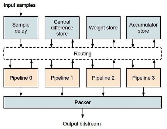
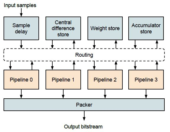
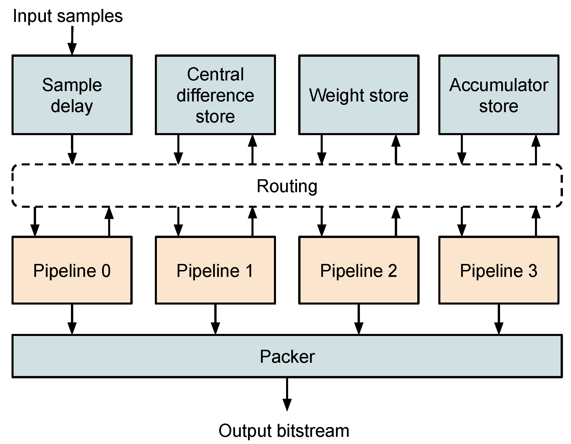
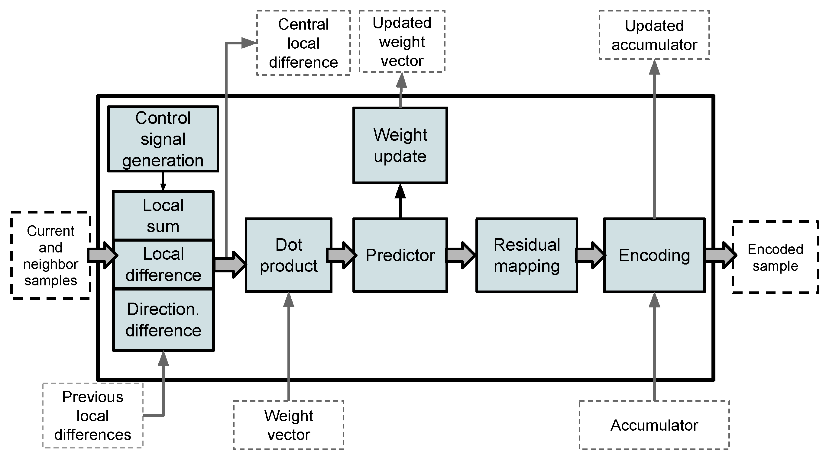
3.1. Pipeline
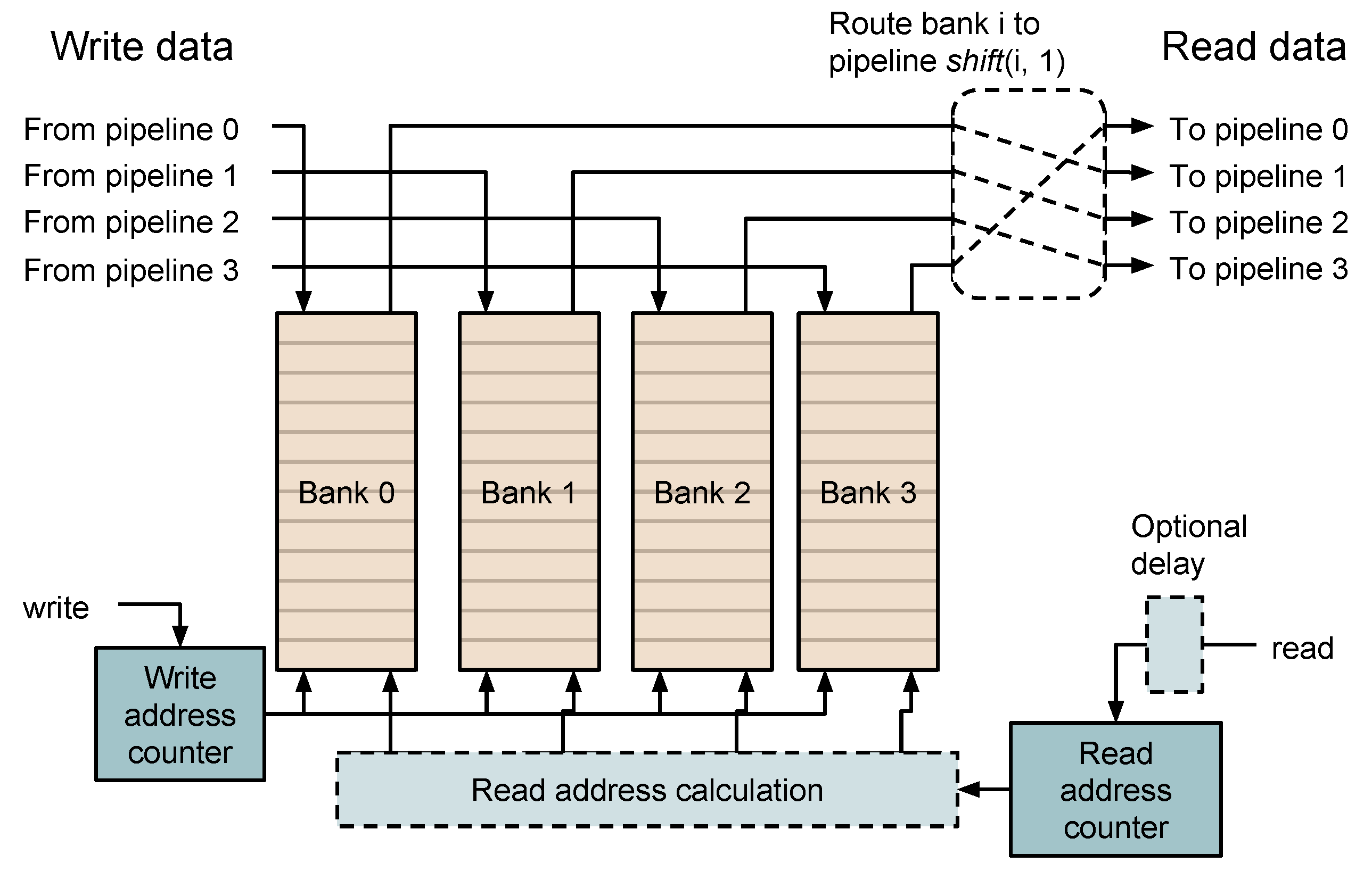
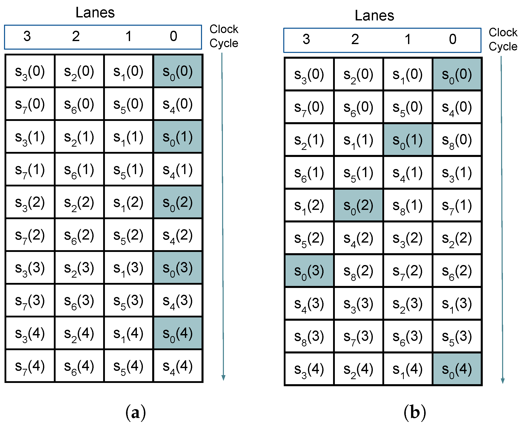
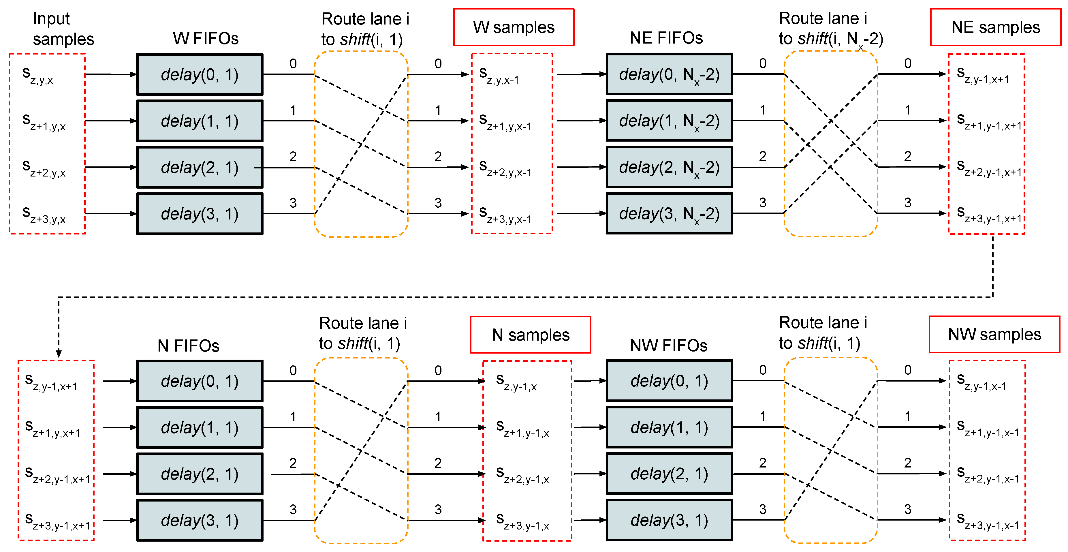
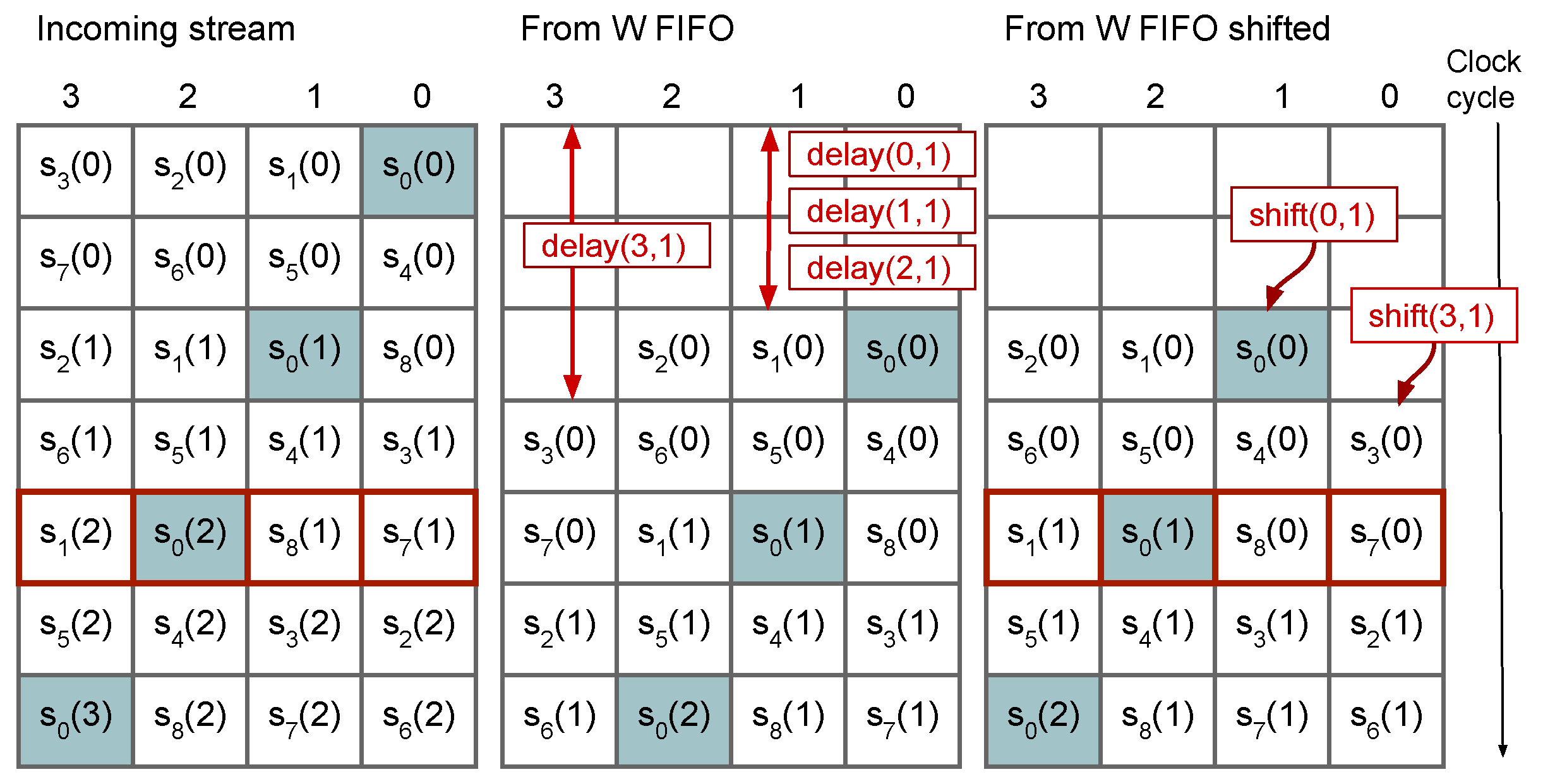
3.2. Sample Delay
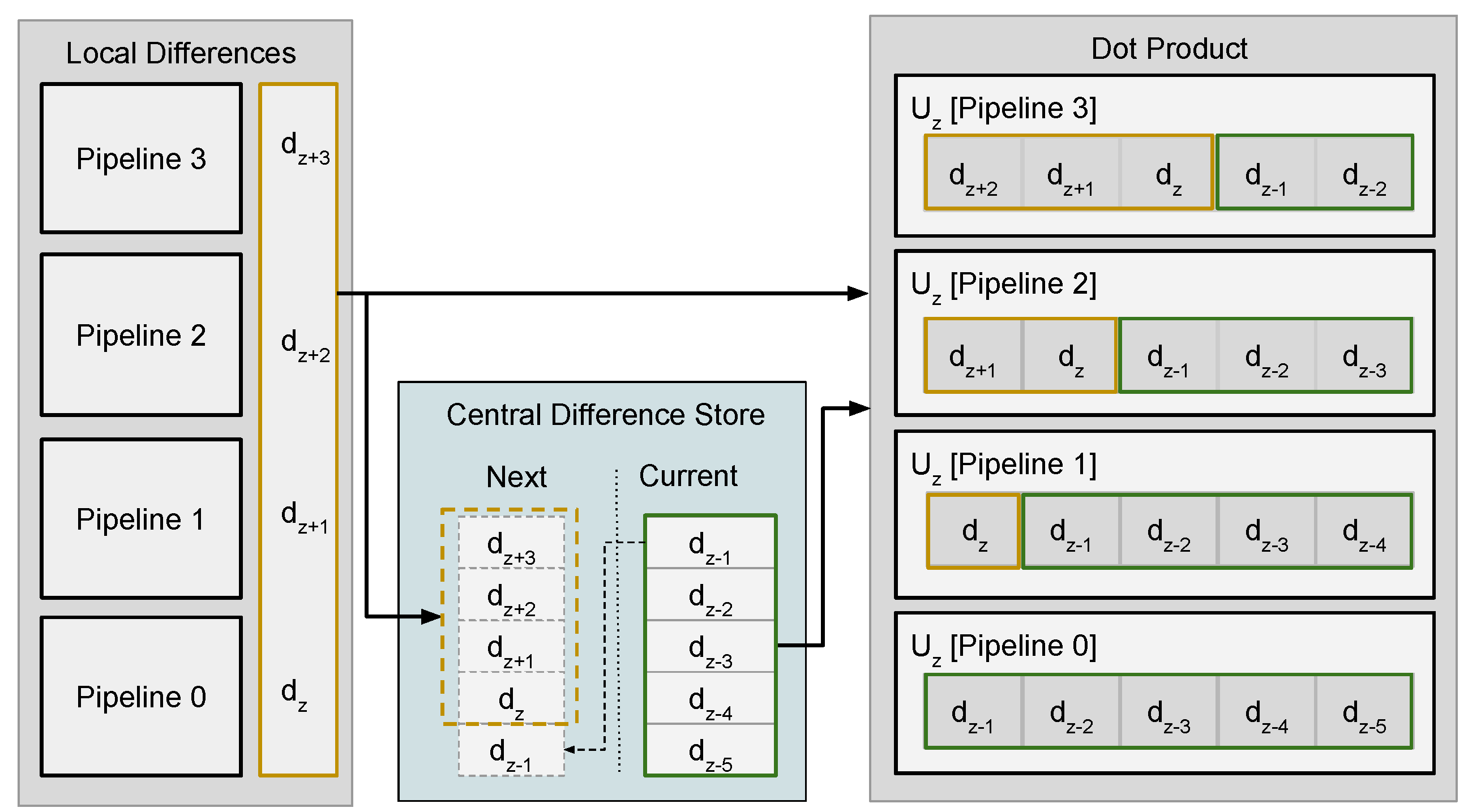
3.3. Local Differences
3.4. Weights and Accumulators
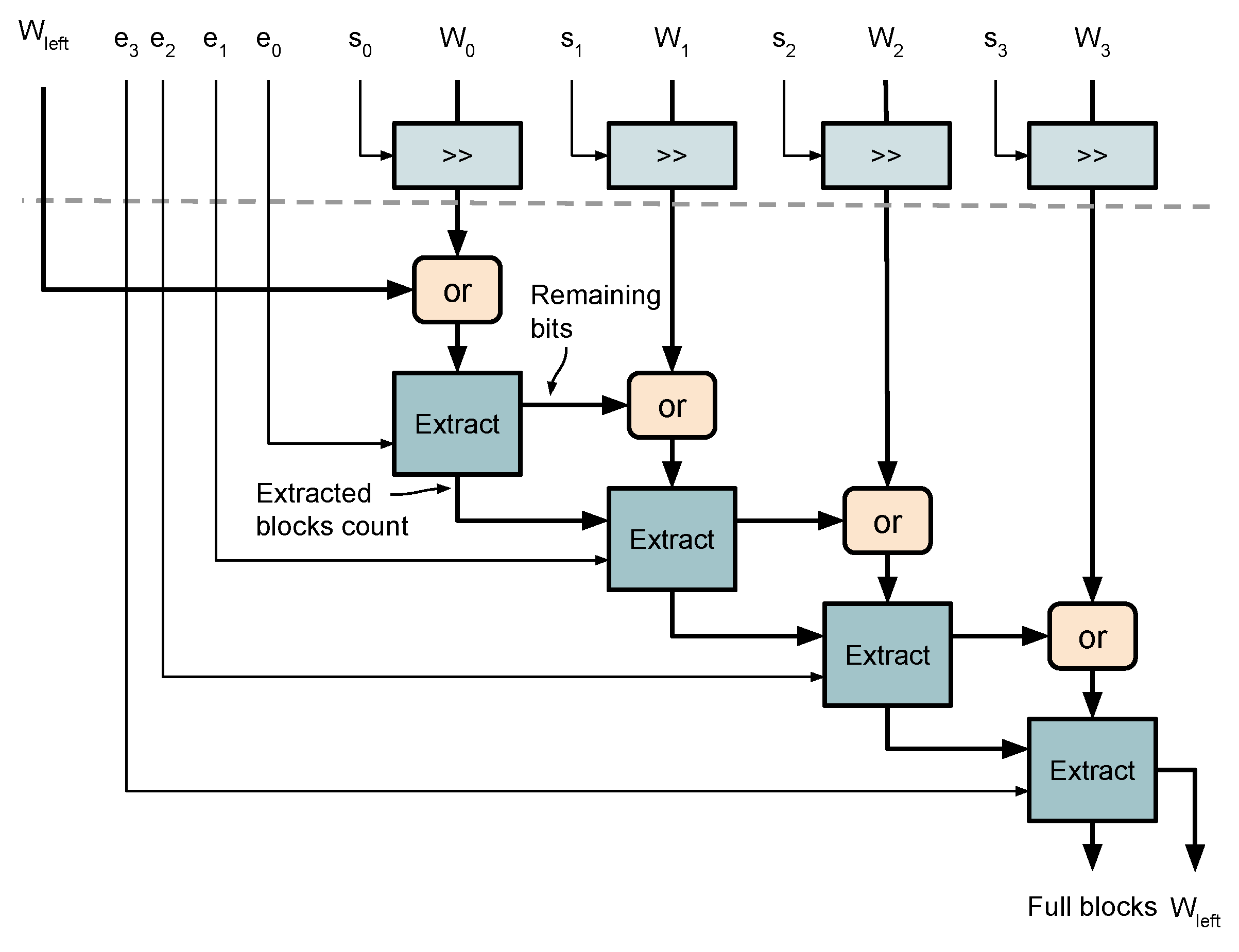
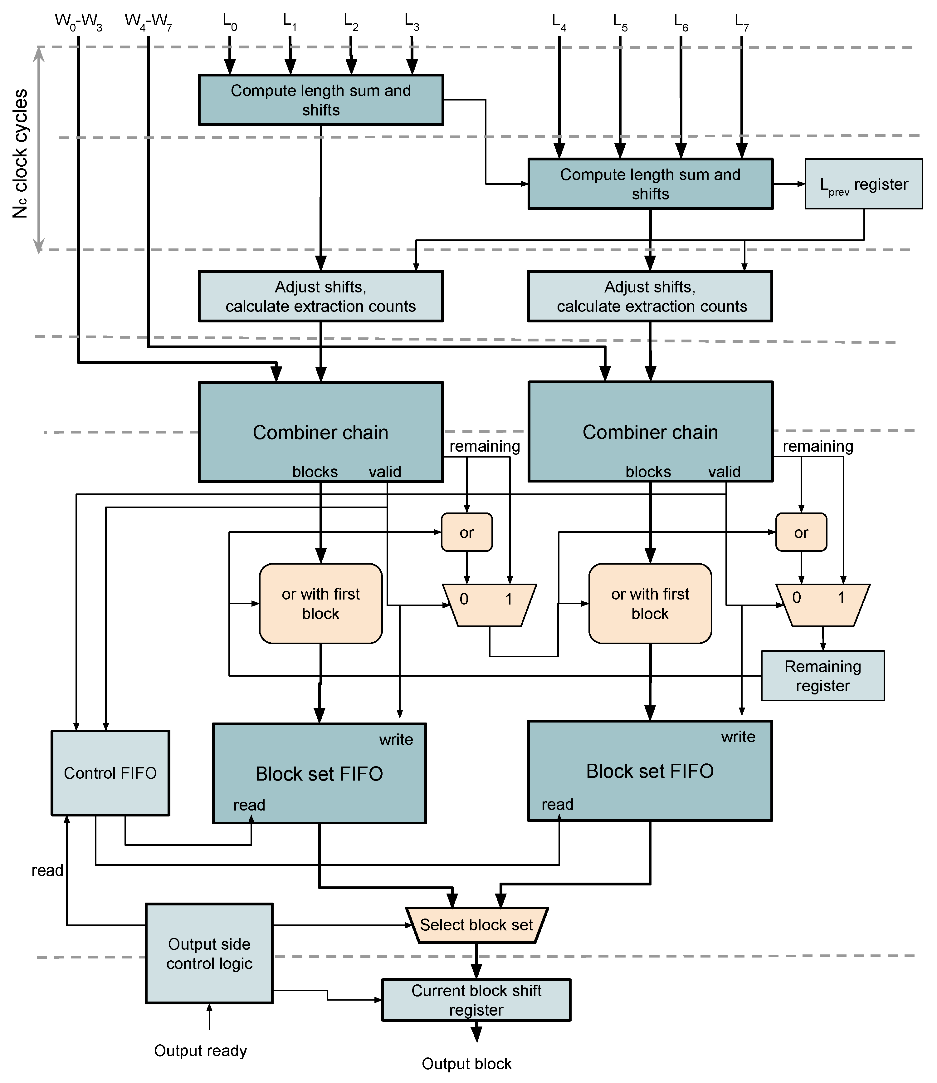
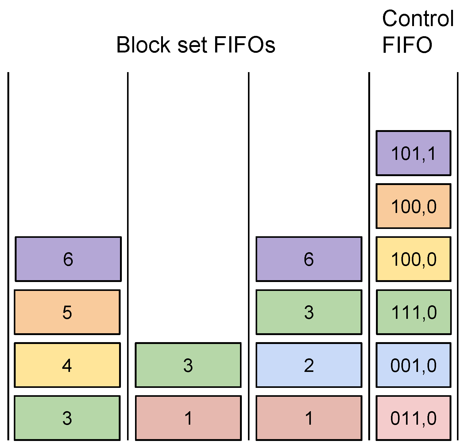
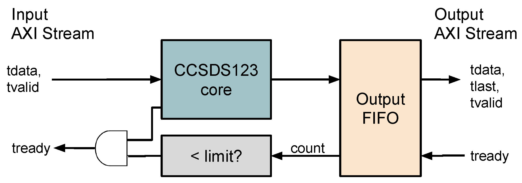
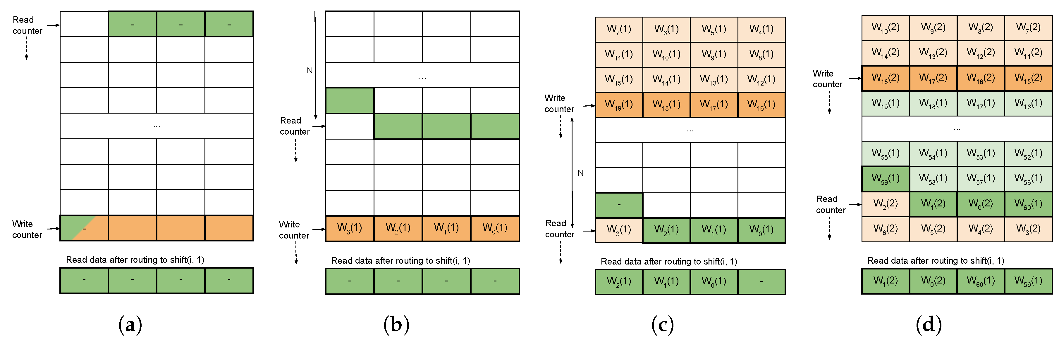
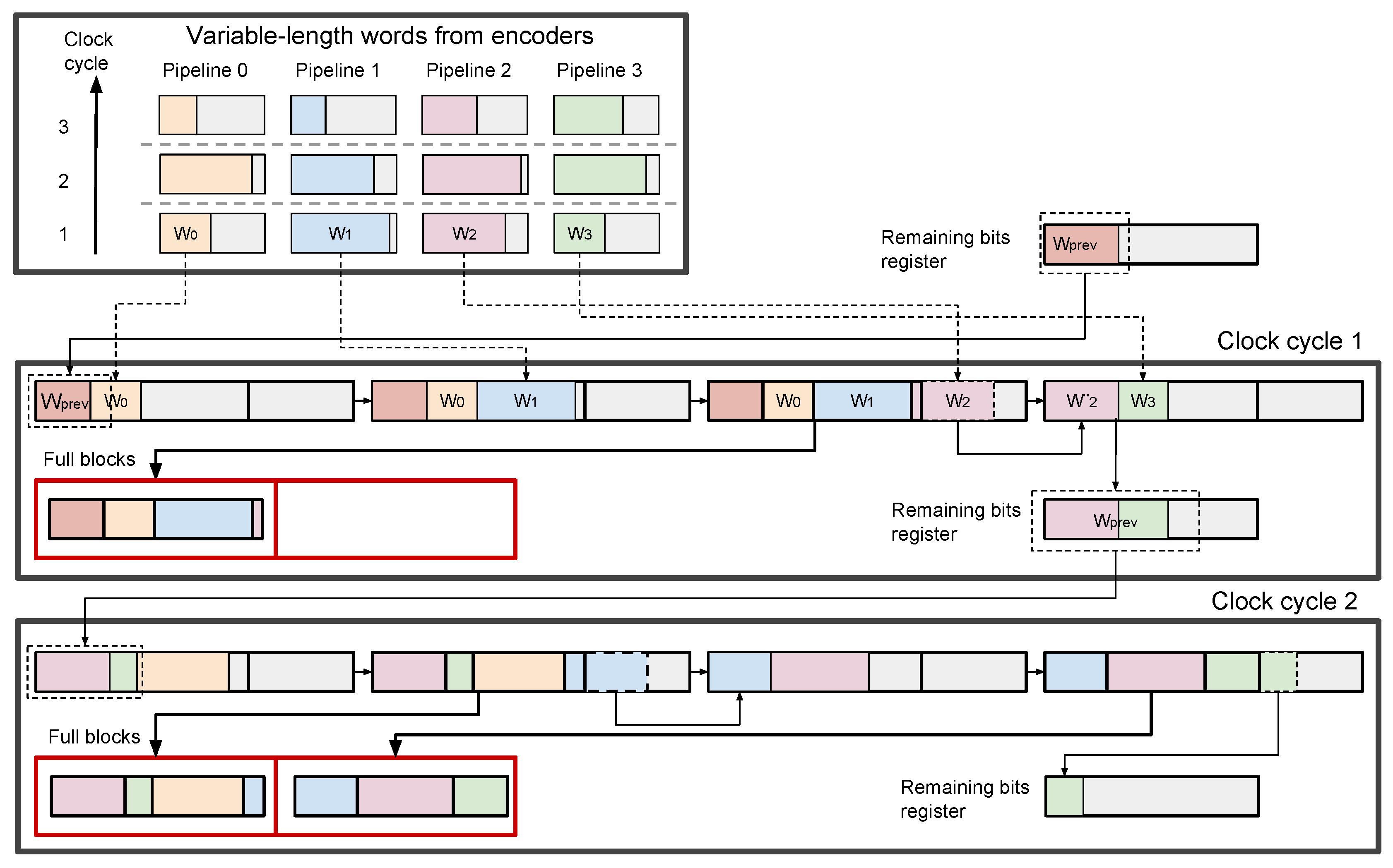
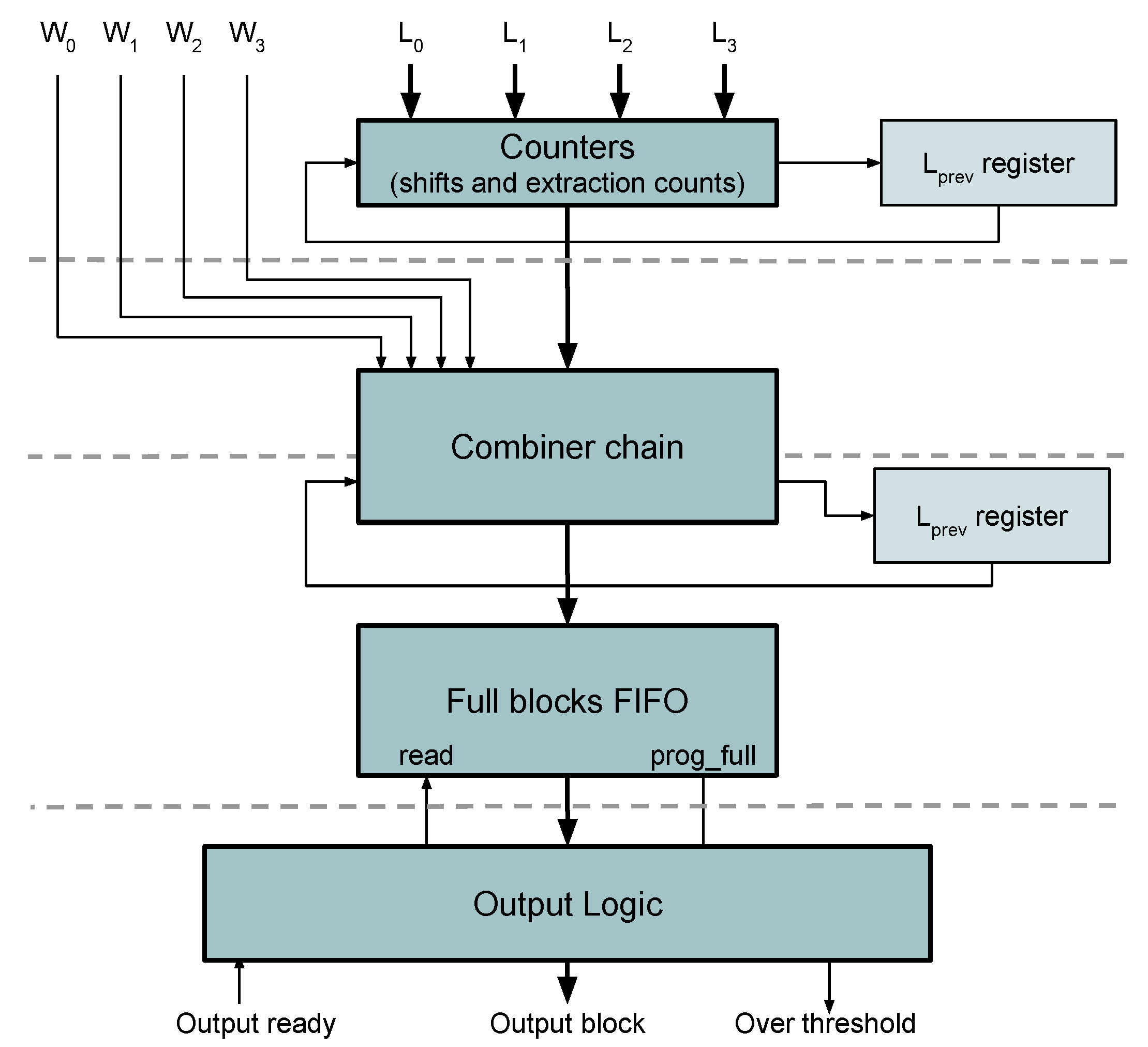
3.5. Packing of Variable Length Words
4. Results
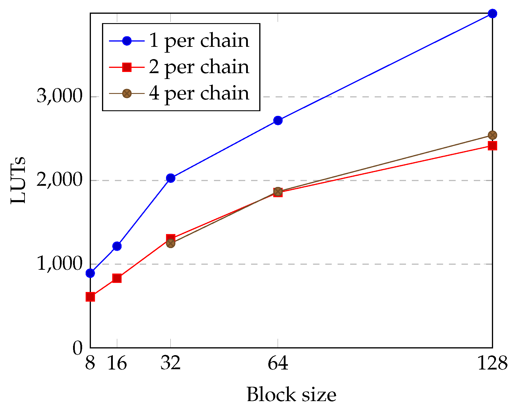
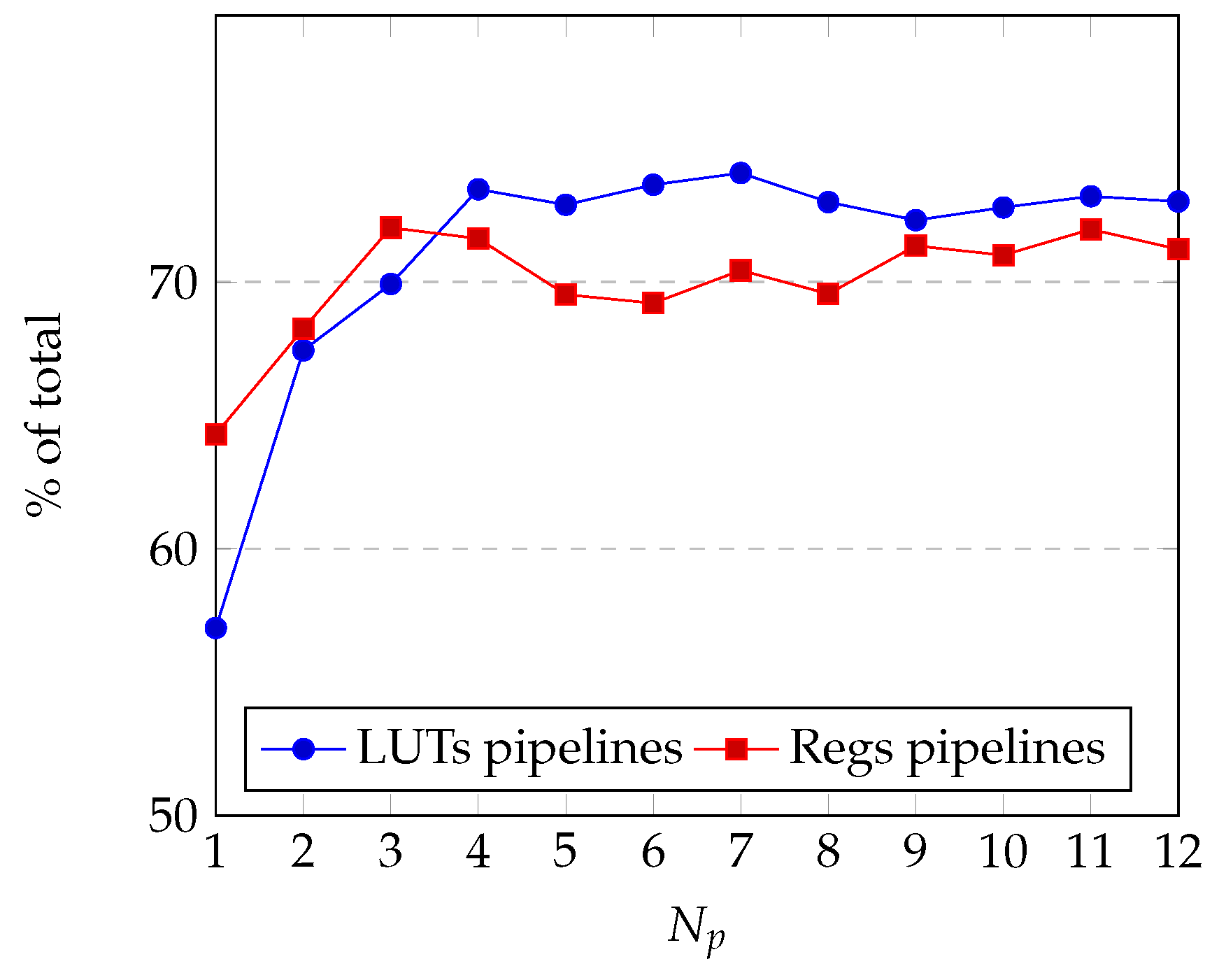
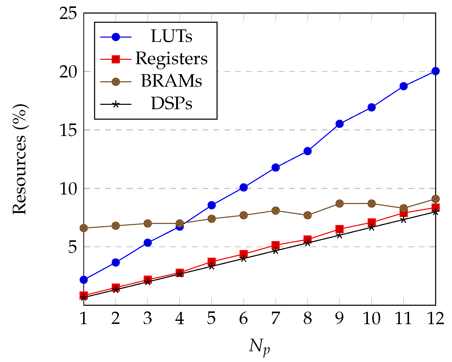
4.1. Utilization Results
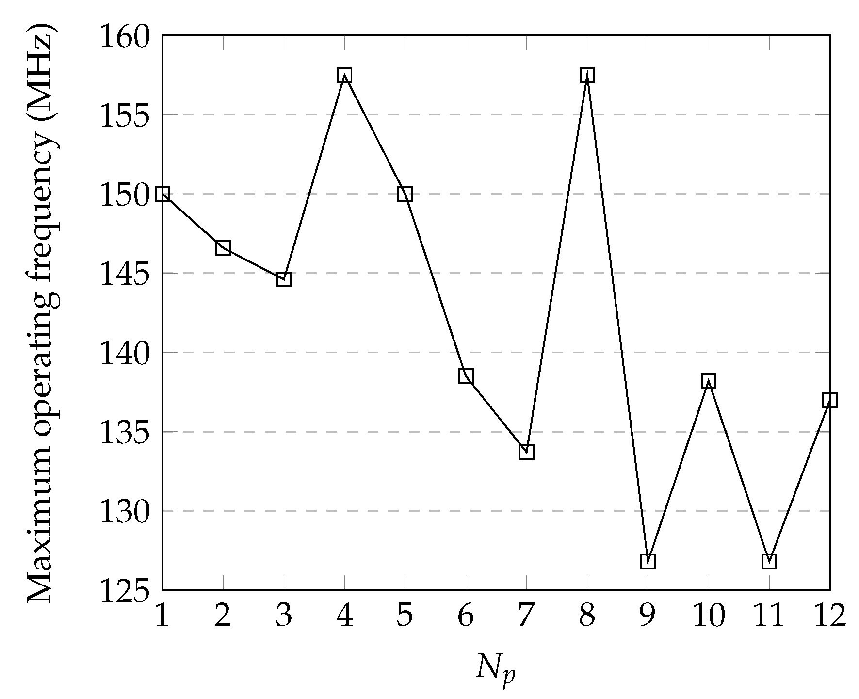
4.2. Timing
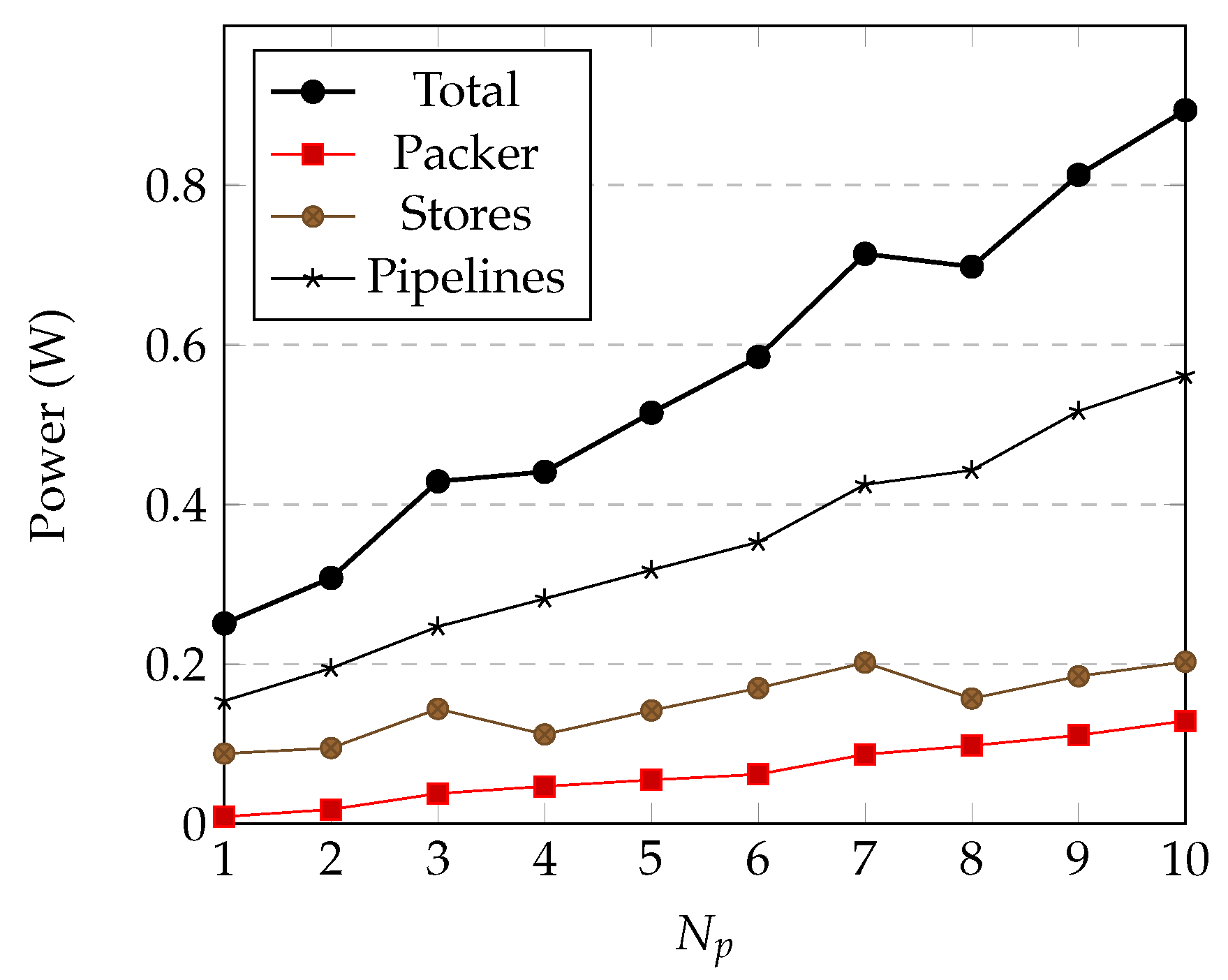
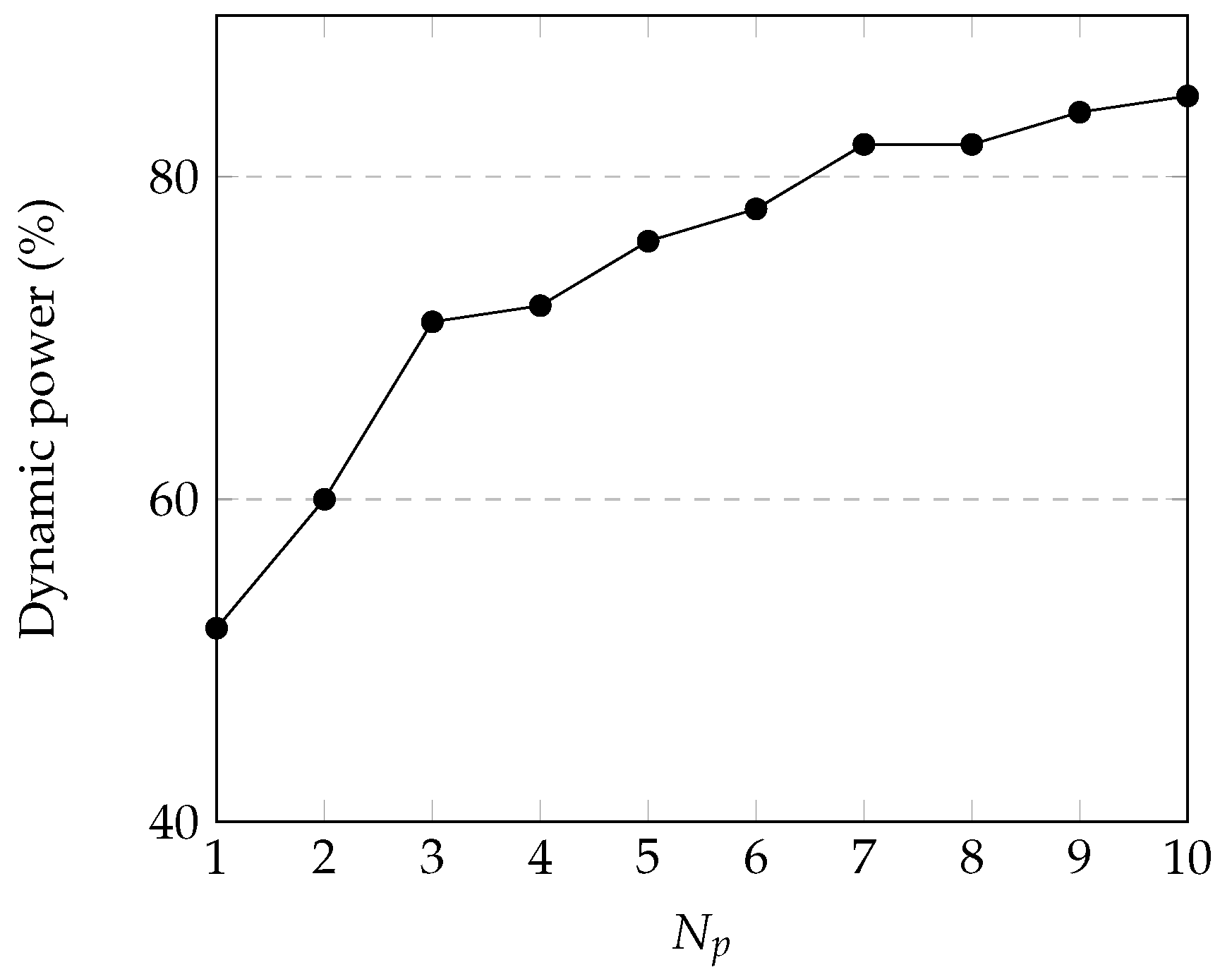
4.3. Power Estimation
4.4. Comparison with State-of-the-Art Implementations
5. Conclusions
Author Contributions
Funding
Conflicts of Interest
References
- George, A.D.; Wilson, C.M. Onboard Processing With Hybrid and Reconfigurable Computing on Small Satellites. Proc. IEEE 2018, 106, 458–470. [Google Scholar] [CrossRef]
- NASA. Moderate Resolution Imaging Spectroradiometer (MODIS). Available online: https://modis.gsfc.nasa.gov/ (accessed on 12 November 2018).
- NASA. Airborne Visible InfraRed Imaging Spectrometer (AVIRIS). Available online: https://aviris.jpl.nasa.gov/ (accessed on 12 November 2018).
- Aires, F.; Chédin, A.; Scott, N.A.; Rossow, W.B. A regularized neural net approach for retrieval of atmospheric and surface temperatures with the IASI instrument. J. Appl. Meteorol. 2002, 41, 144–159. [Google Scholar] [CrossRef]
- Naval Research Laboratory. Hyperspectral Imager for the Coastal Ocean (HICO). Available online: http://hico.coas.oregonstate.edu/ (accessed on 12 November 2018).
- Corson, M.R.; Korwan, D.R.; Lucke, R.L.; Snyder, W.A.; Davis, C.O. The hyperspectral imager for the coastal ocean (HICO) on the international space station. In Proceedings of the IGARSS 2008 IEEE International Geoscience and Remote Sensing Symposium, Boston, MA, USA, 7–11 July 2008; Volume 4. [Google Scholar]
- Soukup, M.; Gailis, J.; Fantin, D.; Jochemsen, A.; Aas, C.; Baeck, P.; Benhadj, I.; Livens, S.; Delauré, B.; Menenti, M.; et al. HyperScout: Onboard Processing of Hyperspectral Imaging Data on a Nanosatellite. In Proceedings of the Small Satellites, System & Services Symposium (4S) Conference, Valletta, Malta, 30 May–3 June 2016. [Google Scholar]
- Consultative Committee for Space Data Systems. Lossless Data Compression-CCSDS 121.0-B-2. In Blue Book; CCSDS Secretariat: Washington, DC, USA, 2012. [Google Scholar]
- Consultative Committee for Space Data Systems. Image Data Compression-CCSDS 122.0-B-1. In Blue Book; CCSDS Secretariat: Washington, DC, USA, 2005. [Google Scholar]
- Consultative Committee for Space Data Systems. Lossless Multispectral and Hyperspectral Image Compression-CCSDS 120.2-G-1. In Green Book; CCSDS Secretariat: Washington, DC, USA, 2015. [Google Scholar]
- Consultative Committee for Space Data Systems. Lossless Multispectral and Hyperspectral Image Compression-CCSDS 123.0-B-1. In Blue Book; CCSDS Secretariat: Washington, DC, USA, 2012. [Google Scholar]
- Keymeulen, D.; Aranki, N.; Bakhshi, A.; Luong, H.; Sarture, C.; Dolman, D. Airborne demonstration of FPGA implementation of Fast Lossless hyperspectral data compression system. In Proceedings of the 2014 NASA/ESA Conference on Adaptive Hardware and Systems (AHS), Leicester, UK, 14–17 July 2014; pp. 278–284. [Google Scholar]
- Santos, L.; Berrojo, L.; Moreno, J.; López, J.F.; Sarmiento, R. Multispectral and hyperspectral lossless compressor for space applications (HyLoC): A low-complexity FPGA implementation of the CCSDS 123 standard. IEEE J. Sel. Top. Appl. Earth Observ. Remote Sens. 2016, 9, 757–770. [Google Scholar] [CrossRef]
- Theodorou, G.; Kranitis, N.; Tsigkanos, A.; Paschalis, A. High Performance CCSDS 123.0-B-1 Multispectral & Hyperspectral Image Compression Implementation on a Space-Grade SRAM FPGA. In Proceedings of the 5th International Workshop on On-Board Payload Data Compression, Frascati, Italy, 28–29 September 2016; pp. 28–29. [Google Scholar]
- Báscones, D.; González, C.; Mozos, D. FPGA Implementation of the CCSDS 1.2.3 Standard for Real-Time Hyperspectral Lossless Compression. IEEE J. Sel. Top. Appl. Earth Observ. Remote Sens. 2017, 11, 1158–1165. [Google Scholar] [CrossRef]
- Báscones, D.; González, C.; Mozos, D. Parallel Implementation of the CCSDS 1.2.3 Standard for Hyperspectral Lossless Compression. Remote Sens. 2017, 9, 973. [Google Scholar] [CrossRef]
- University of Las Palmas de Gran Canaria, Institute for Applied Microelectronics (IUMA). SHyLoC IP Core. Available online: http://www.esa.int/Our_Activities/Space_Engineering_Technology/Microelectronics/SHyLoC_IP_Core (accessed on 12 November 2018).
- Tsigkanos, A.; Kranitis, N.; Theodorou, G.A.; Paschalis, A. A 3.3 Gbps CCSDS 123.0-B-1 Multispectral & Hyperspectral Image Compression Hardware Accelerator on a Space-Grade SRAM FPGA. IEEE Trans. Emerg. Top. Comput. 2018. [Google Scholar] [CrossRef]
- Fjeldtvedt, J.; Orlandić, M.; Johansen, T.A. An Efficient Real-Time FPGA Implementation of the CCSDS-123 Compression Standard for Hyperspectral Images. IEEE J. Sel. Top. Appl. Earth Observ. Remote Sens. 2018, 11, 3841–3852. [Google Scholar] [CrossRef]
- Augé, E.; Sánchez, J.E.; Kiely, A.B.; Blanes, I.; Serra-Sagristà, J. Performance impact of parameter tuning on the CCSDS-123 lossless multi-and hyperspectral image compression standard. J. Appl. Remote Sens. 2013, 7, 074594. [Google Scholar] [CrossRef]
- GICI Group, Universitat Autonoma de Barcelona. Emporda Software. Available online: http://www.gici.uab.es (accessed on 12 November 2018).
- ARM. AMBA AXI and ACE Protocol Specification; Technical Report; ARM, 2011; Available online: http://infocenter.arm.com/help/topic/com.arm.doc.ihi0022d (accessed on 12 November 2018).
- Xilinx. 7 Series FPGAs Configurable Logic Block User Guide; Technical Report; Xilinx: San Jose, CA, USA, 2016. [Google Scholar]
- Lewis, M.D.; Gould, R.; Arnone, R.; Lyon, P.; Martinolich, P.; Vaughan, R.; Lawson, A.; Scardino, T.; Hou, W.; Snyder, W.; et al. The Hyperspectral Imager for the Coastal Ocean (HICO): Sensor and data processing overview. In Proceedings of the OCEANS 2009, MTS/IEEE Biloxi-Marine Technology for Our Future: Global and Local Challenges, Biloxi, MS, USA, 26–29 October 2009; pp. 1–9. [Google Scholar]
- Consultative Committee for Space Data Systems. Low-Complexity Lossless and Near-lossless Multispectral and Hyperspectral Image Compression-CCSDS 123.0-B-2. In Blue Book; CCSDS Secretariat: Washington, DC, USA, 2019. [Google Scholar]
- Kiely, A.; Klimesh, M.; Blanes, I.; Ligo, J.; Magli, E.; Aranki, N.; Burl, M.; Camarero, R.; Cheng, M.; Dolinar, S.; et al. The new CCSDS Standard for Low-Complexity Lossless and Near-Lossless Multispectral and Hyperspectral Image Compression. In Proceedings of the ESA On-Board Payload Data Compression Workshop (OBPDC), Matera, Italy, 20–21 September 2018. [Google Scholar]


| Model | D | LUTs | Regs | RAM | |||
|---|---|---|---|---|---|---|---|
| SFSI | 12 | 496 | 140 | 240 | 9416 | 8730 | 46 |
| MSG | 10 | 3712 | 3712 | 11 | 7984 | 8133 | 16 |
| MODIS | 12 | 1354 | 2030 | 17 | 8859 | 8682 | 12 |
| M3-Target | 12 | 640 | 2843 | 260 | 10,824 | 8827 | 64 |
| M3-Global | 12 | 320 | 28,283 | 386 | 11,351 | 9086 | 48 |
| Landsat | 8 | 1024 | 1024 | 8 | 6583 | 7410 | 7 |
| Hyperion | 12 | 256 | 3242 | 242 | 9640 | 8888 | 28 |
| Crism-FRT | 12 | 640 | 510 | 545 | 12,882 | 9313 | 130 |
| Crism-HRL | 12 | 320 | 480 | 545 | 12,646 | 9130 | 68 |
| Crism-MSP | 12 | 64 | 2700 | 74 | 8803 | 8843 | 6 |
| CASI | 12 | 405 | 2852 | 72 | 8922 | 8960 | 16 |
| AVIRIS | 16 | 614 | 512 | 224 | 12,033 | 10,696 | 71 |
| AIRS | 14 | 90 | 135 | 1501 | 12,191 | 8569 | 68 |
| IASI | 12 | 66 | 60 | 8461 | - | - | - |
| HICO | 16 | 512 | 2000 | 128 | 11,589 | 10,661 | 35 |
| LUTS | ||||||
|---|---|---|---|---|---|---|
| Pipeline | Sample Store | Accum Store | Weight Store | Packer | Total | |
| 1 | 2137 | 468 | 112 | 504 | 526 | 3747 |
| 2 | 4247 | 672 | 128 | 366 | 884 | 6297 |
| 3 | 6435 | 866 | 196 | 566 | 1139 | 9202 |
| 4 | 8499 | 856 | 180 | 366 | 1665 | 11,566 |
| 5 | 10,723 | 1029 | 230 | 464 | 2263 | 14,709 |
| 6 | 12,765 | 1226 | 272 | 555 | 2513 | 17,331 |
| 7 | 15,005 | 1458 | 317 | 647 | 2826 | 20,253 |
| 8 | 16,550 | 1802 | 350 | 731 | 3238 | 22,671 |
| 9 | 19,297 | 2042 | 397 | 815 | 4131 | 26,682 |
| 10 | 21,191 | 1886 | 440 | 923 | 4668 | 29,108 |
| 11 | 23,584 | 2186 | 416 | 1014 | 5008 | 32,208 |
| 12 | 25,136 | 2268 | 454 | 1112 | 5455 | 34,425 |
| Registers | Block RAM | ||||||||
|---|---|---|---|---|---|---|---|---|---|
| Pipeline | Samp. Store | Acc. Store | Weig. Store | Packer | Total | Samp. Store | Packer | Total | |
| 1 | 1856 | 156 | 36 | 152 | 687 | 2887 | 32 | 1 | 33 |
| 2 | 3532 | 238 | 56 | 280 | 1069 | 5175 | 32 | 2 | 34 |
| 3 | 5394 | 351 | 78 | 410 | 1255 | 7488 | 33 | 2 | 35 |
| 4 | 6869 | 440 | 98 | 546 | 1636 | 9589 | 32 | 3 | 35 |
| 5 | 8921 | 540 | 120 | 670 | 2579 | 12,830 | 32.5 | 4.5 | 37 |
| 6 | 10,424 | 648 | 142 | 814 | 3033 | 15,061 | 33 | 5.5 | 38.5 |
| 7 | 12,460 | 756 | 164 | 951 | 3358 | 17,689 | 35 | 5.5 | 40.5 |
| 8 | 13,455 | 808 | 184 | 1085 | 3810 | 19,342 | 32 | 6.5 | 38.5 |
| 9 | 15,994 | 909 | 206 | 1209 | 4094 | 22,412 | 36 | 7.5 | 43.5 |
| 10 | 17,311 | 1000 | 228 | 1332 | 4507 | 24,378 | 35 | 8.5 | 43.5 |
| 11 | 19,546 | 1100 | 250 | 1476 | 4784 | 27,156 | 33 | 8.5 | 41.5 |
| 12 | 20,479 | 1200 | 272 | 1611 | 5189 | 28,751 | 36 | 9.5 | 45.5 |
| Implementation | Order | P | D | Platform | Throughput | Power | ||
|---|---|---|---|---|---|---|---|---|
| [MHz] | [MSa/s] | [Mb/s] | [mW] | |||||
| AVIRIS-NG [3] | - | - | 14 | Sensor Max. | - | 30.72 | 430 | - |
| HICO [5,24] | - | - | 14 | Sensor Max. | - | 4.78 | 66.92 | - |
| Keymeulen et al. [12] | BIP | 3 | 13 | Virtex-5 (FX130T) | 40 | 40 | 520 | - |
| HyLoC, Santos et al. [13] | BSQ | 3 | 16 | Virtex-5 (FX130T) | 134 | 11.2 | 179 | 1488 |
| Theodorou et al. [14] | BIP | 3 | 16 | Virtex-5 (FX130T) | 110 | 110 | 1790 | - |
| Bascones et al. [15] | BIP | 0–15 | 16 | Virtex-7 | 50 | 47.6 | 760 | 450 |
| Bascones et al. [16]— | BIP | 0–15 | 16 | Virtex-5 (FX130T) | - | 179.7 | 3040 | |
| Bascones et al. [16]— | BIP | 0–15 | 16 | Virtex-7 | - | 219.4 | 3510.4 | 5300 |
| SHyLoC, Santos et al. [17] | All | 0–15 | 16 | Virtex-5 (FX130T) | 140 | 140 | 2240 | - |
| Tsigkanos et al. [18] | BIP | 3 | 16 | Virtex-5 (FX130T) | 213 | 213 | 3300 | 4720 |
| Fjeldtvedt et al. [19] | BIP | 0–15 | 16 | Zynq-7000 | 147 | 147 | 2350 | 295 |
| Proposed work— | BIP | 0–15 | 16 | Zynq-7000 | 157 | 624 | 9984 | 440 |
| Proposed work— | BIP | 0–15 | 16 | Zynq-7000 | 150 | 750 | 12,000 | 515 |
© 2019 by the authors. Licensee MDPI, Basel, Switzerland. This article is an open access article distributed under the terms and conditions of the Creative Commons Attribution (CC BY) license (http://creativecommons.org/licenses/by/4.0/).
Share and Cite
Orlandić, M.; Fjeldtvedt, J.; Johansen, T.A. A Parallel FPGA Implementation of the CCSDS-123 Compression Algorithm. Remote Sens. 2019, 11, 673. https://doi.org/10.3390/rs11060673
Orlandić M, Fjeldtvedt J, Johansen TA. A Parallel FPGA Implementation of the CCSDS-123 Compression Algorithm. Remote Sensing. 2019; 11(6):673. https://doi.org/10.3390/rs11060673
Chicago/Turabian StyleOrlandić, Milica, Johan Fjeldtvedt, and Tor Arne Johansen. 2019. "A Parallel FPGA Implementation of the CCSDS-123 Compression Algorithm" Remote Sensing 11, no. 6: 673. https://doi.org/10.3390/rs11060673
APA StyleOrlandić, M., Fjeldtvedt, J., & Johansen, T. A. (2019). A Parallel FPGA Implementation of the CCSDS-123 Compression Algorithm. Remote Sensing, 11(6), 673. https://doi.org/10.3390/rs11060673