Article

An Imaging Algorithm for Multireceiver Synthetic Aperture Sonar

1
College of Electrical and Information Engineering, Lanzhou University of Technology, Lanzhou 730050, China
2
Laboratory of Underwater Acoustics, Zhanjiang 524022, China
3
Aerodynamics Research and Development Center, Computational Aerodynamics Institute, Mianyang 621000, China
4
Naval Research Academy, Beijing 102249, China
*
Author to whom correspondence should be addressed.
Remote Sens. 2019, 11(6), 672; https://doi.org/10.3390/rs11060672
Submission received: 20 February 2019 / Revised: 13 March 2019 / Accepted: 17 March 2019 / Published: 20 March 2019
(This article belongs to the Special Issue Radar and Sonar Imaging and Processing)

Abstract

:
For the multireceiver synthetic aperture sonar (SAS), the point target reference spectrum (PTRS) in the two-dimensional (2D) frequency domain and azimuth modulation in the range Doppler domain were first deduced based on a numerical evaluation method and accurate time delay. Then, the difference between the PTRS and azimuth modulation generated the coupling term in the 2D frequency domain. Compared with traditional methods, the PTRS, azimuth modulation and coupling term was better at avoiding approximations. Based on three functions, an imaging algorithm is presented in this paper. Considering the fact that the coupling term is characterized by range variance, the range-dependent sub-block processing method was exploited to perform the decoupling. Simulation results showed that the presented method improved the imaging performance across the whole swath in comparison with existing multireceiver SAS processor. Furthermore, real data was used to validate the presented method.

1. Introduction

Synthetic aperture sonar (SAS) [1] provides high resolution images via the coherent processing of successive echo data along the virtual aperture. This makes SAS a suitable technique for applications such as searching for small objects [2], imaging of wrecks [3], underwater archaeology [4] and pipeline inspection [5]. Additionally, it improves the classification and detection of objects based on SAS images [6]. Multireceiver SAS [7], as opposed to monostatic SAS constellation, offers a fast mapping rate at a given resolution. However, it does this at the cost of complicated signal processor.
For the multireceiver SAS, the point target reference spectrum (PTRS) [8] is a prerequisite of fast imaging algorithms. The two-way slant range of the multireceiver SAS consists of two hyperbolic range histories, which include the instantaneous range between the moving transmitter and target and that between the target and moving receiver. The two hyperbolic range histories make it difficult to deduce the point of stationary phase (PSP) and PTRS using the method of stationary phase [9]. In order to solve this problem, approximations are often exploited. In [10,11,12], the phase center approximation (PCA) was used to model a transducer located at the midpoint between the transmitter and receiver. With this, the echo data of multiple receivers is converted into the monostatic format. However, the preprocessing includes the compensation of phase errors [13]. Due to the space variance of approximation errors [13], it is difficult to compensate phase errors completely. Loffeld et al. [14] have presented an analytic PTRS. Their method was based on the approximation that the transmitter and receiver contribute equally to the Doppler frequency. Based on the method of stationary phase [9], two PSPs corresponding to the transmitter’s phase and receiver’s phase were deduced. The phase history of the transmitter and that of the receiver were expanded into a power series at their individual PSPs. Both phases were then combined to generate a quadratic function. It can be found that two approximations are exploited by this method. One is the equal Doppler contribution of the transmitter and receiver, and the other is the Taylor approximation of the transmitter’s phase and receiver’s phase. In general, this method only applies to the narrow beam case [14,15]. There are still some other methods deducing the analytic PTRS. The basic idea relies on series approximation. In [16], the quadratic approximation of the two-way range was exploited. This introduced a large residual error, which degraded the imaging performance at close range. Moreover, this method did not consider the compensation of the stop-and-hop error [12]. A single target suffers from the coordinate deviation in azimuth [17]. However, a distributed target suffers from the distortion. In [18,19], the two-way range was expanded into a power series with respect to the slow time. Additionally, the PSP was expanded into a power series based on the series reversion method. The accuracy of the two-way range and PSP was limited by the number of terms in the polynomial. With this method, the series approximation was used twice. The approximation error increased with the slow time. The accumulative error would be large when the SAS system works with the wide beam case. In [20,21], the instantaneous Doppler wavenumber was exploited to deduce the analytic PTRS. The two-way slant range was formulated as a function of equivalent bistatic squint angle and half bistatic angle [20,21]. Based on the method of stationary phase [9], the azimuth wavenumber can also be expressed as a function of equivalent bistatic squint angle and half bistatic angle. Then, the PTRS was expressed as a function of half bistatic angle, which should be analytically calculated. Considering that the triangle whose vertices were the transmitter, receiver and target, the fourth order equation with respect to half bistatic angle was obtained based on the theorem of sine and some basic algebra skills. In [21], this equation was solved using the series reversion method [18,19]. The accuracy of the PTRS is also limited by the number of terms in the power series.
Using an accurate time delay of the transmitted signal [12], the back projection (BP) algorithm [22] can provide high resolution results. In this paper, we present an imaging algorithm, which was also based on the accurate time delay of the transmitted signal. With the numerical evaluation method [23], we first calculated the PSP and azimuth PSP. The PTRS and azimuth modulation can be easily obtained based on their respective numerical PSPs. Then, we obtained the coupling term in the two-dimensional (2D) frequency domain using the phase difference between the numerical PTRS and azimuth modulation. The PTRS, coupling term and azimuth modulation avoiding approximations were further exploited to develop the imaging processor, which compensated the coupling phase based on the sub-block processing method.
This paper is organized as follows. In Section 2, the imaging geometry and signal model are introduced. Section 3 introduces the PTRS, azimuth modulation and coupling term based on the numerical evaluation method. Section 4 presents the imaging algorithm based on three functions. Section 5 compares the presented method with traditional methods, and highlights the advantages of the presented method. In Section 6, processing results of the simulated data and real data are used to validate the presented method. Finally, some conclusions are reported in the last section.

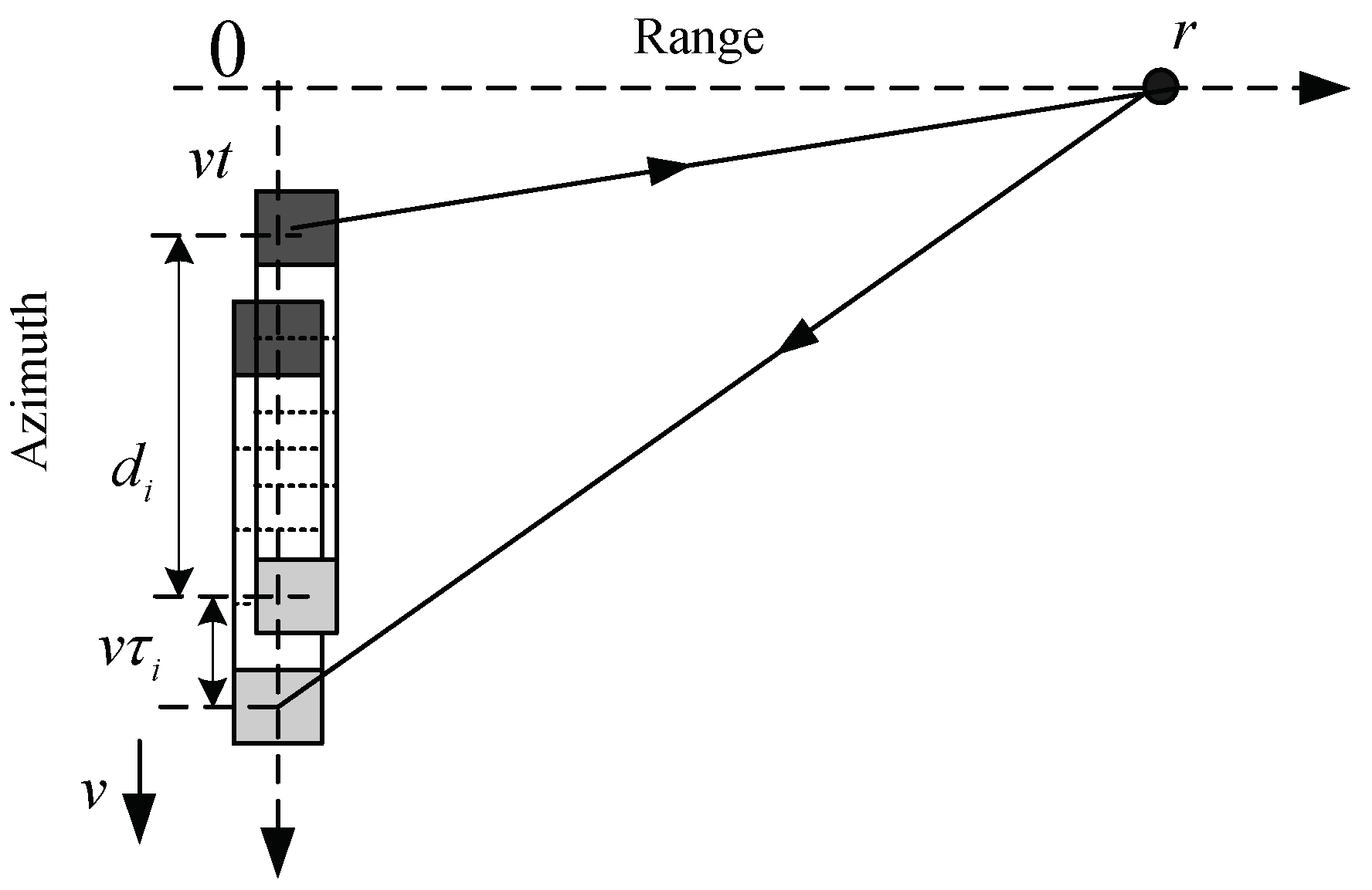
2. Imaging Geometry and Signal Model

The imaging geometry of the multireceiver SAS is shown in Figure 1. The linear array consists of a transmitter and receiver array including M uniformly spaced receivers. In Figure 1, the black rectangle denotes the transmitter. Each receiver has an integer index i [ 1 , M ] . For the i-th receiver, the distance between the receiver and transmitter is denoted by d i . The linear array is aligned in the sonar moving direction, which is called the azimuth dimension. The horizontal direction represents the range dimension. Since the SAS configuration shown in Figure 1 is characterized by azimuth invariance, an ideal point target located at coordinates (r, 0) is used. t denotes the slow time in the azimuth dimension. The fast time in the range dimension is represented by τ . c is the sound speed in water. v represents the velocity of the sonar platform.
In Figure 1, the two-way slant range is from the transmitter to target and then back to the i-th receiver. When the transmitter moves to the position v t , a chirp signal p ( τ ) is transmitted. The accurate time delay [12] of the echo signal corresponding to the i-th receiver is given by:
τ i = v ( v t + d i ) + c v 2 t 2 + r 2 c 2 v 2 + [ v ( v t + d i ) + c v 2 t 2 + r 2 ] 2 + ( c 2 v 2 ) ( 2 v t d i + d i 2 ) c 2 v 2
In (1), we consider the forward distance of the i-th receiver during the signal reception, because the sonar is continuously travelling along the azimuth dimension [17]. After demodulation, the echo signal corresponding to the i-th receiver is expressed as:
s s i ( τ , t ) = p ( τ τ i ) ω a ( t ) exp { j 2 π f c τ i }
where f c is the center frequency. The composite beam pattern corresponding to the i-th receiver and transmitter is represented by ω a ( ) . For simplicity, we neglect this beam pattern to concentrate on the phase processing.

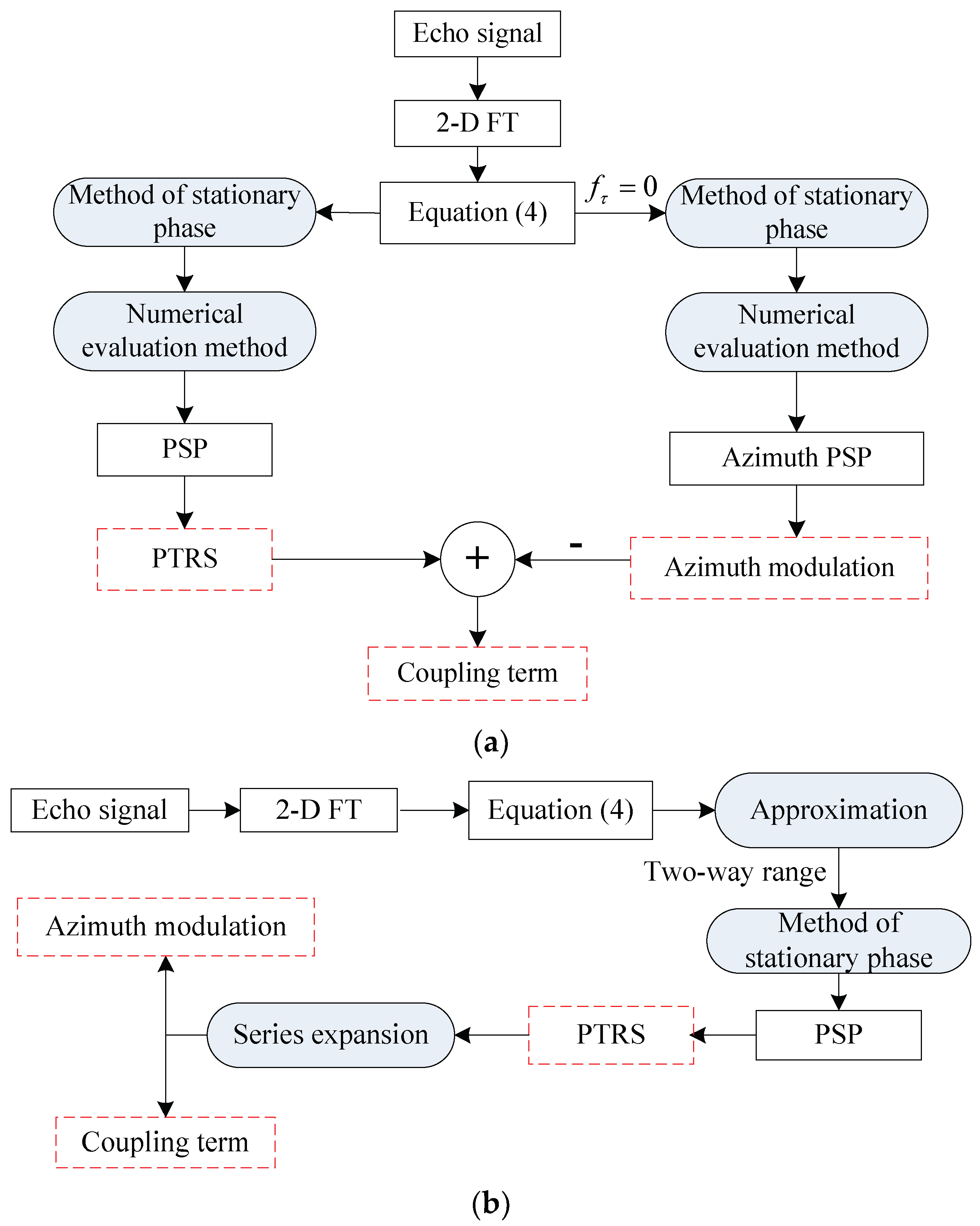
3. PTRS, Azimuth Modulation and Coupling Term

The BP algorithm [22] should compute the instantaneous range from the moving transmitter to target and then back to moving receiver. Therefore, (1) is very suitable for the BP algorithm. Since (1) considers the influence of stop-and-hop assumption, BP algorithm can provide high resolution image. However, (1) cannot be used by traditional fast algorithms. For simplicity, the forward distance of the i-th receiver during the signal reception is approximated by v τ i 2 v r / c . This approximation degrades the imaging performance when the SAS system works with the wide beam case. In this paper, the accurate time delay shown as (1) is extended to fast imaging algorithms. The PTRS, azimuth modulation and coupling term play an important role in developing fast imaging algorithms. We start from the deduction of the PTRS, azimuth modulation and coupling term in this section.

3.1. PTRS

Based on the Fourier transformation (FT), the signal denoted by (2) is transformed into the 2D frequency domain. The expression is given by:
S S i ( f τ , f t ) = P ( f τ ) T s / 2 T s / 2 exp { j 2 π ( f c + f τ ) τ i j 2 π f t t } d t
where T s denotes the integration time; P ( f τ ) is the spectrum of the transmitted signal; f τ and f t are the instantaneous and Doppler frequencies.
Due to the complex expression of (1), it is difficult to calculate (3). To solve this problem, approximations are usually exploited by traditional methods. However, the residual errors would influence the imaging performance. Here, we present the numerical result, which avoids approximations.
The phase of the exponent in (3) is defined as:
Ψ i ( f τ , f t ) = 2 π ( f c + f τ ) τ i 2 π f t t
Applying the method of stationary phase [9] to (4) yields:
τ i ( t ˜ i ) t + f t f c + f τ = 0
where t ˜ i [ T s / 2 , T s / 2 ] represents the PSP; τ i t denotes the first derivative with respect to the slow time.
Using (1), the first derivative with respect to the slow time is given by:
τ i t = v 2 + c t v 2 [ ( v t ) 2 + r 2 ] 0.5 c 2 v 2 + { { v [ ( v t ) + d i ] + c ( v t ) 2 + r 2 } 2 + ( c 2 v 2 ) [ 2 ( v t ) d i + d i 2 ] } 0.5 c 2 v 2 × { [ v 2 t + v d i + c ( v t ) 2 + r 2 ] { v 2 + c t v 2 [ ( v t ) 2 + r 2 ] 0.5 } + v d i ( c 2 v 2 ) }
(5) cannot be solved analytically, as (6) is very complicated. Due to this, the numerical evaluation method is used to calculate the effective solution of (5). The effective solution called the PSP is denoted by t ˜ i . Substituting the numerical PSP into (4) yields:
Ψ i ( f τ , f t ; t ˜ i ) = 2 π ( f c + f τ ) τ i ( t ˜ i ) 2 π f t t ˜ i
Examining (7), we see that the numerical PTRS avoids approximations. Besides, the PTRS is a function of the instantaneous frequency f τ , Doppler frequency f t and range r. The space variance makes the development of fast imaging algorithms a challenge.
Based on the series expansion, the PTRS is decomposed into the azimuth modulation and coupling term. Using the coupling term, the decoupling operation between the range and azimuth dimensions is first carried out, and hence the imaging process is decomposed into two separate filtering processes in the range and azimuth dimensions. However, it is hard to obtain both terms using series expansion, because (7) is not an analytic expression.

3.2. Azimuth Modulation

After the decoupling operation, the azimuth compression is usually performed in the range Doppler domain. It is easily concluded that the filtering function related to the azimuth compression is only a function of the range r and Doppler frequency f t [8,9]. In other words, the azimuth modulation is independent of the instantaneous frequency f τ [8,9]. If the azimuth modulation were obtained, the phase difference between the PTRS and azimuth modulation denotes the coupling term. In other words, the azimuth modulation should be first derived. For conventional methods, the azimuth modulation and coupling term are simultaneously obtained based on the series approximation of the PTRS with respect to the instantaneous frequency. Inspecting (7), it is impossible to perform the series approximation, because the PTRS in this paper does not possess the explicit expression. To solve this problem, the numerical evaluation method is still used to calculate the azimuth modulation. Since the azimuth modulation is independent of the instantaneous frequency [8,9], we obtain the azimuth modulation by setting f τ = 0 in (7). This is given by:
φ a c _ i ( f t ; r ) = Ψ i ( f τ , 0 ; t ^ i ) = 2 π f c τ i ( t ^ i ) 2 π f t t ^ i
In (8), t ^ i [ T s / 2 , T s / 2 ] represents the PSP used by the azimuth modulation. At this point, we call it the azimuth PSP. It is independent of the instantaneous frequency [8,9]. Although we present the azimuth modulation in (8), the azimuth PSP is not expressed explicitly. Considering the fact that the azimuth modulation is independent of the instantaneous frequency, we turn our attention to the deduction of the azimuth PSP. Setting f τ = 0 in (5) yields:
τ i ( t ^ i ) t + f t f c = 0
Based on the numerical method, the azimuth PSP t ^ i is calculated. Substituting the azimuth PSP into (8), we obtain the numerical expression of the azimuth modulation.

3.3. Coupling Term

Because of the relative motion between the sonar and target, the distance between them changes with time; hence, the time delay changes correspondingly. The effect is that the received echo from the same target at different azimuth sample times will distribute at different bins along the range direction. This phenomenon is called the range cell migration (RCM), which completely describes the coupling between the range and azimuth dimensions. Due to the coupling, the imaging process cannot be simply decomposed into two separate filtering processes in the range and azimuth dimensions. The direct processing scheme is to cancel the coupling before the azimuth matched filtering.
With traditional methods, the coupling term is obtained by using the series expansion of the PTRS with respect to the instantaneous frequency. Since the PTRS shown as (7) does not own an explicit expression, the series expansion method cannot be exploited. In practice, the PTRS consists of the coupling term and azimuth modulation. Therefore, the difference between the PTRS and azimuth modulation denotes the coupling term between the range and azimuth dimensions. It is expressed as:
φ i ( f τ , f t ; r ) = Ψ i ( f τ , f t ; r ) φ a c _ i ( f t ; r )
Until now, the PTRS, coupling term and azimuth modulation are all deduced. The azimuth modulation is a wideband signal. After decoupling, the matched filtering is expected to perform the focusing in the azimuth dimension.

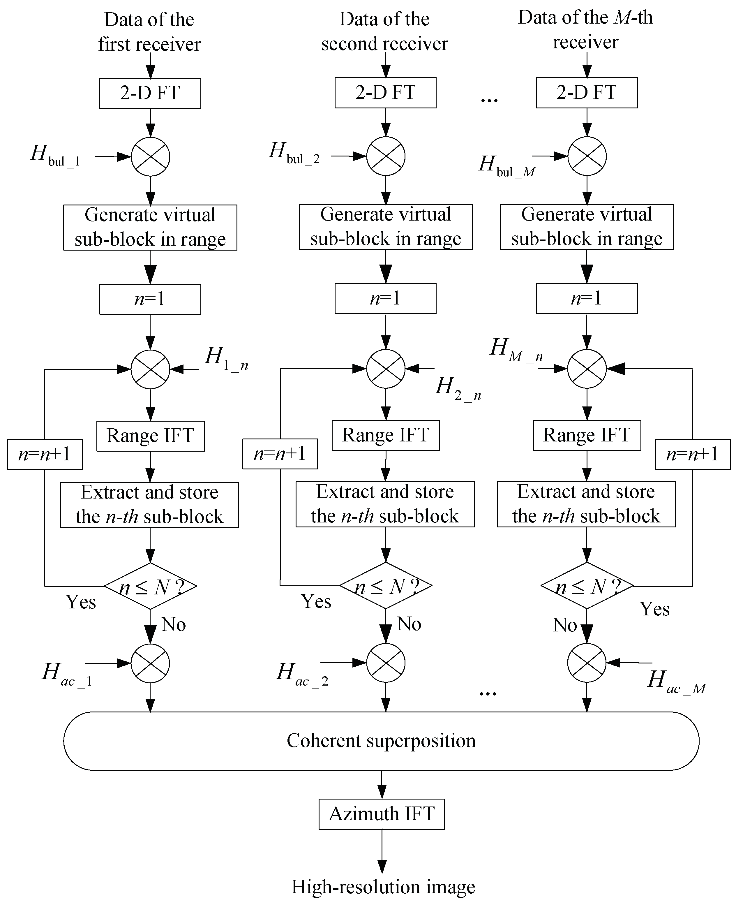
4. Imaging Algorithm

The key issue of the SAS imagery is the decoupling. Inspecting (10), the coupling phase is a function of the range, instantaneous frequency and Doppler frequency. Due to the range variance, we cannot perform the decoupling operation in the range Doppler domain. Based on the characteristic of the coupling phase, the sub-block processing method is used to perform the decoupling operation. In this section, important steps of the presented method are introduced in detail.

4.1. 2D FT

In this step, each receiver’s data is transformed into 2D frequency domain based on the FT. Each receiver data is undersampling. The energy of the frequency f t [ P R F / 2 , P R F / 2 ] is a combination of all the energy related to the frequency points ( ,   f t P R F ,   f t ,   f t + P R F ,   ) [ M P R F / 2 , M P R F / 2 ] . Here, f t [ P R F / 2 , P R F / 2 ] denotes the Doppler frequency related to the sampling rate of each receiver’s data. In other words, the spectrum in the Doppler domain is aliased M times. Here the pulse repetition frequency is denoted by PRF, which is also the sampling frequency of each receiver’s data in the azimuth dimension. The alias can be suppressed by the coherent processing of multireceiver data.

4.2. Decoupling

The coupling phase shown as (10) is characterized by range variance. Although the coupling phase is accurate, it is hard to compensate the coupling phase completely. Here, the sub-block processing method is exploited to perform the decoupling operation. Since it is hoped that the echo signal of a target is in the same range cell (usually at r), the range deviation from its desired position denotes the RCM. Based on (10), the RCM in the 2D frequency domain is expressed as:
φ de _ i ( f τ , f t ; r ) = φ i ( f τ , f t ; r ) 4 π f τ r c
From (11), we see that the RCM is a function of the range, instantaneous frequency and Doppler frequency. Based on this characteristic, the sub-block processing method rather than interpolation is exploited to carry out the range cell migration correction (RCMC). The decoupling is decomposed into two steps. One is the bulk decoupling, and the other is the differential decoupling. Based on (11), the filtering function of the bulk decoupling is given by:
H bul _ i = conj { P ( f τ ) } exp { j φ de _ i ( f τ , f t ; r c ) }
where r c represents the center range of the mapping swath; conj ( ) represents the complex conjugate.
The bulk decoupling simultaneously performs the range matched filtering. Considering targets at reference range, the coupling is completely removed after this step. However, other targets suffer from the residual error, which is φ de _ i ( f τ , f t ; r ) φ de _ i ( f τ , f t ; r c ) . Based on the sub-block processing method, the differential decoupling is used to solve this problem. Before performing the differential decoupling, the whole swath is virtually segmented into N sub-blocks in the range direction. Based on (11) and (12), the filtering function of the differential decoupling is written as
H i _ n = exp { j φ de ( f τ , f t ; r ref _ n ) j φ de _ i ( f τ , f t ; r c ) }
where the center range of the n-th sub-block is used as the reference range, which is denoted by r ref _ n . The variable n [ 1 , N ] denotes the sub-block index.
Based on (13), we remove the coupling between the range and azimuth dimensions for the data of the n-th sub-block. Then, the data is transformed into the time domain via the inverse Fourier transformation (IFT) in the range direction. For each sub-block, the differential decoupling is carried out using (13). The processed sub-blocks are extracted and stored in the range Doppler domain. The coupling between the range and azimuth dimensions is cancelled when N sub-blocks are reckoned into a new signal matrix.

4.3. Azimuth Compression

The sonar transmits and receives signals and then stores the received signal. This process is conducted at a set of locations along the moving trajectory. The signal collected at these locations forms different units of synthetic aperture called azimuth sample serials. By processing the data collected within the synthetic aperture time, an equivalent large sonar array can be obtained. By coherently processing the echo data, we obtain the high resolution in the azimuth dimension.
In practice, the azimuth echo of the SAS system can also be regarded as a wideband signal. The matched filter can still be used to compress the azimuth signal. According to the theory of the matched filter [9], it is necessary to set parameters of the matched filter to be the same as Doppler parameters of the azimuth signal. As a result, parameters should be adjusted at different ranges in order to get high resolution in azimuth across the whole swath. This is the main difference between the range compression and azimuth compression.
Inspecting (8), the azimuth modulation only depends on the range r and Doppler frequency f t . It is not a function of the instantaneous frequency f τ any more. This term is responsible for the azimuth matched filtering after performing the decoupling between the range and azimuth dimensions. Considering the new signal matrix in the range-Doppler domain, the azimuth compression is directly carried out based on the azimuth modulation. The filtering function is given by:
H a c _ i = exp { j φ a c _ i ( f t ; r ) }
After this step, the signal is compressed in azimuth. However, the azimuth spectrum of each receiver’s data is aliased M times due to the (1/M)-th undersampling.

4.4. Coherent Superposition

Monostatic SAS system has a transducer, which is used as the transmitter and receiver at different times. The wide swath in range requires a low rate of P R F . However, the high resolution in azimuth requires high rate of P R F . In other words, the different requirements of the pulse repetition frequency in range and azimuth dimensions lead to a trade-off between swath width and azimuth resolution.
To solve this issue, the multireceiver SAS including a transmitter and receiver array is used. When the sampling of each individual receiver occurs at a rate of P R F , the effective sampling of the equivalent monostatic system is M P R F . After transmitting a pulse, M samples can be recorded. Based on the PCA method [12], the unambiguous spectrum satisfying the Nyquist rate is recovered before the SAS imagery. With the PCA method, the PTRS of multireceiver SAS is decomposed into two parts. One depends on d i . The other is independent of d i , and it is similar to the PTRS of monostatic SAS. When it comes to recover the unambiguous spectrum, the phase related to d i must be simultaneously compensated. The subsequent processing can be done with the help of imaging algorithms based on monostatic SAS system. With the presented method, the PTRS cannot be decomposed into aforementioned two parts. According to the theory of the linear time invariant system [9], we can exchange the processing order between the SAS imagery and recovery of the unambiguous spectrum. In other words, each receiver’s data can be focused before recovering the unambiguous spectrum. Considering each receiver’s data, we obtain focusing results in the range Doppler domain by using the decoupling and azimuth compression. Since each receiver’s data is sampled by the pulse repetition frequency P R F , the spectrum of a single receiver data must be aliased. Fortunately, the coherent processing of multireceiver data can suppress this alias. The spectrums of all receiver data are coherently superposed in the range Doppler domain. The resultant data would satisfy the Nyquist rate in azimuth, and the equivalent sampling rate is M P R F . The high resolution image is obtained after an azimuth IFT.
According to the presented steps, the block diagram of the proposed algorithm is shown in Figure 2.

5. Comparison with Traditional Methods

In this section, we begin with the comparison of the PTRS, which is the basis of fast imaging algorithms. To directly use the method of stationary phase [9], the series expansion of the two-way slant range is often used by traditional methods [12,16,19]. From Figure 1, the two-way slant range can be formulated as:
R i ( t ; r ) = c τ i = r 2 + ( v t ) 2 + r 2 + ( v t + v τ i + d i ) 2
where r 2 + ( v t ) 2 denotes the instantaneous range between the target and transmitter, and r 2 + ( v t + v τ i + d i ) 2 is the instantaneous range between the i-th receiver and target. Here, v τ i represents the forward distance during the signal reception. Considering the complex expression of the accurate time delay, v τ i is often approximated by 2 v r / c for simplicity.
(15) is the sum of two square roots, which make it difficult to acquire the PTRS based on the method of stationary phase [9]. To solve this problem, (15) is expanded into a power series, which is given by:
R i ( t ; r ) q = 0 Q k i _ q t q
where k-coefficients in (16) can be calculated by the rule of series expansion [9]. To obtain the analytical PSP, the parameter Q often satisfies 2 Q 4 .
Inspecting (16), the series expansion would lead to the approximation error. Besides, the error of stop-and-hop approximation is not completely compensated. Since the presented method is based on the accurate time delay, both issues are successfully avoided.
We now discuss the link of the SAS imagery between the presented method and traditional methods [12,16,19]. Expanding the PTRS as a Taylor series with respect to the instantaneous frequency, various imaging algorithms are developed. The second order series approximation is exploited by the range-Doppler (R-D) algorithm [24] and chirp scaling (CS) algorithm [25]. The nonlinear CS algorithm [26,27] and quartic phase algorithm [28] are based on the third and fourth order approximation, respectively. The range migration algorithm (RMA) [29,30] requires that the PTRS is a linear function of the range. Generally, the series approximation of the PTRS is unavoidable if traditional fast algorithms were still exploited. Based on traditional methods, we conclude that the azimuth modulation is independent of the instantaneous frequency. With this characteristic, we first derive the azimuth modulation by setting f τ = 0 in (7). Then, the difference between the PTRS and azimuth modulation denotes the coupling term. Consequently, the Taylor expansion of the PTRS is avoided. Based on (7), (8) and (10), the block diagram related to the deduction of the PTRS, coupling term and azimuth modulation is shown in Figure 3a. The dashed rectangle in Figure 3a denotes important terms deduced by the presented method. Figure 3b shows the deduction of traditional methods. It can be found that traditional methods are very tedious. In this paper, we provide a novel aspect for the accurate deduction of the PTRS, azimuth modulation and coupling term.
In general, our method owns two major advantages. Traditional fast imaging methods cannot directly use the accurate time delay, which is often exploited by the BP algorithm. Approximations are usually used to deduce the PTRS, azimuth modulation and coupling term. Unfortunately, the approximations degrade the imaging performance. In this paper, the PTRS, azimuth modulation and coupling term are deduced based on the accurate time delay. Consequently, these functions avoid approximations. It is the first advantage of the presented method.
The second advantage is that our imaging scheme can be simply extended to any other PTRS. The presented imaging scheme does not require the series expansion of the PTRS with respect to the instantaneous frequency. With the presented method, the key step is to deduce the azimuth modulation. Considering the analytic PTRS, the azimuth modulation can be directly obtained by setting f τ = 0 in the PTRS. When the PTRS is complicated, the azimuth modulation is deduced by using two steps. The first step should calculate the azimuth PSP by setting f τ = 0 in PSP. The subsequent step sets f τ = 0 in the PTRS and substitutes the azimuth PSP into the PTRS. Based on the PTRS and azimuth modulation, the coupling term can be calculated. After carrying out the decoupling operation based on the sub-block processing method, the imaging process is decomposed into two separate filtering processes in the range and azimuth dimensions.

6. Simulations and Real Data Processing

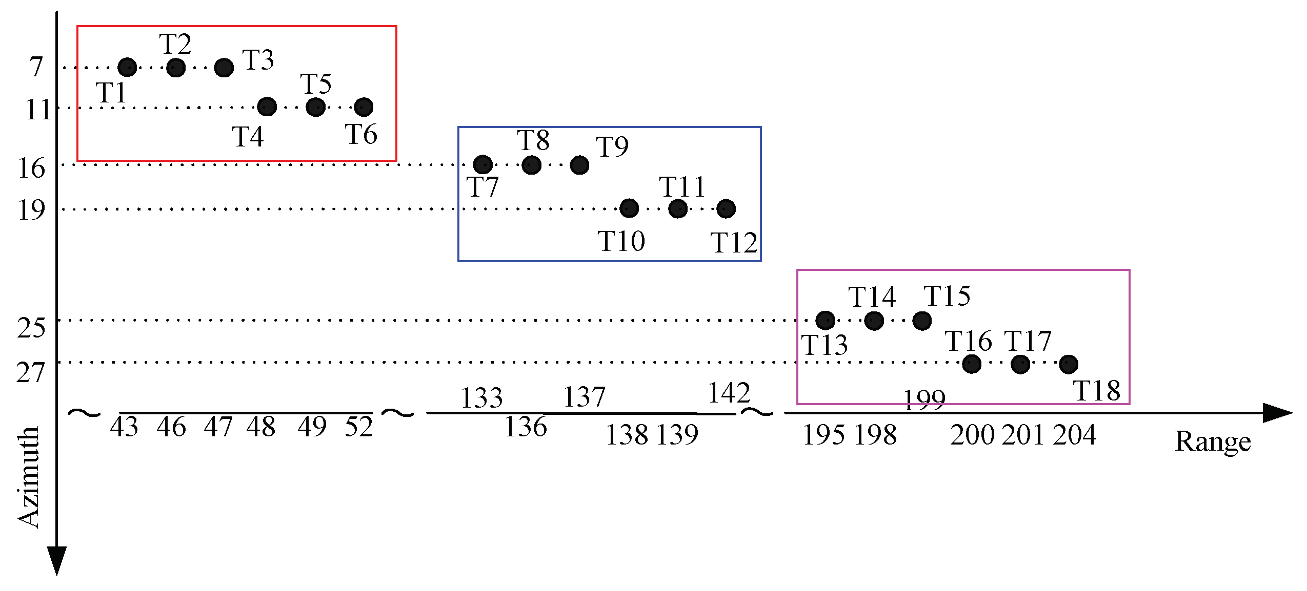
6.1. Simulation Results

In this section, simulations are exploited to validate the presented method. The SAS parameters are listed in Table 1.

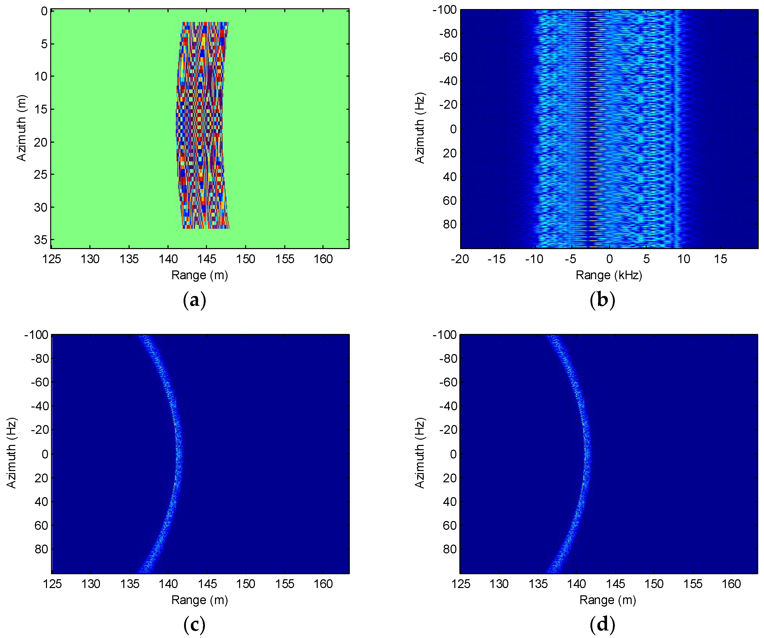
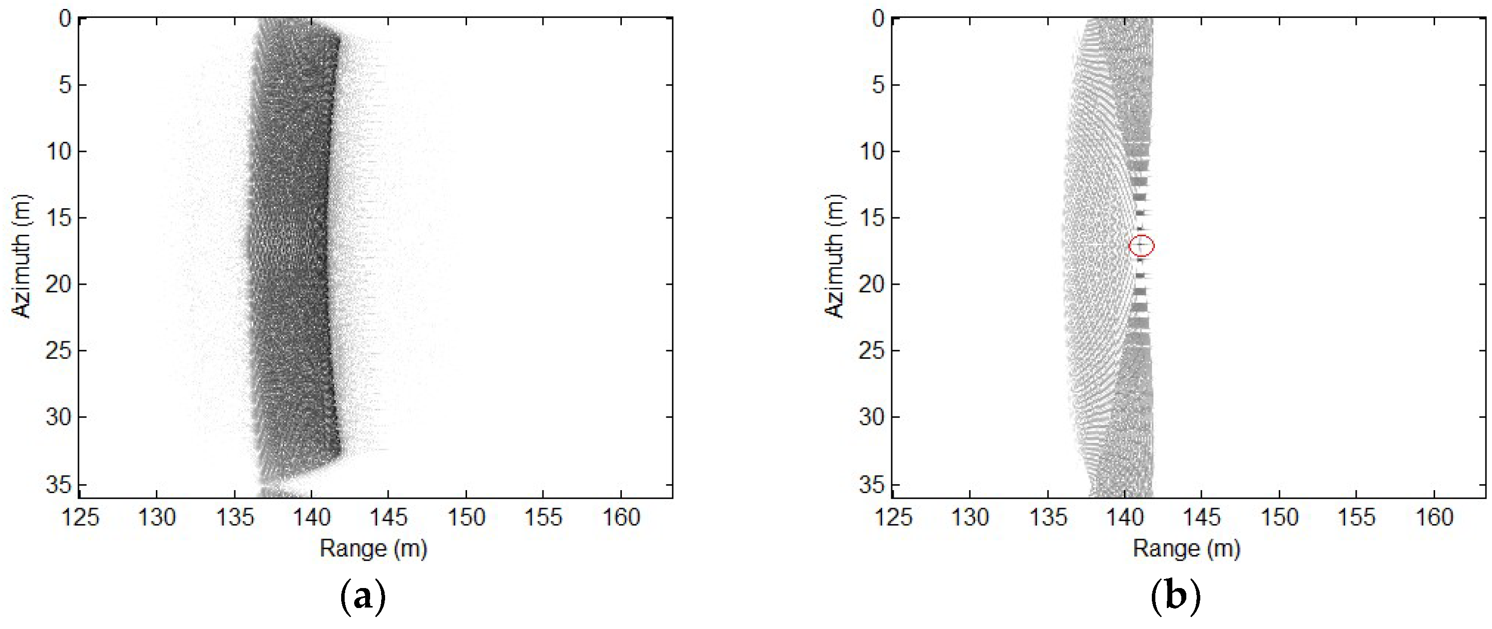
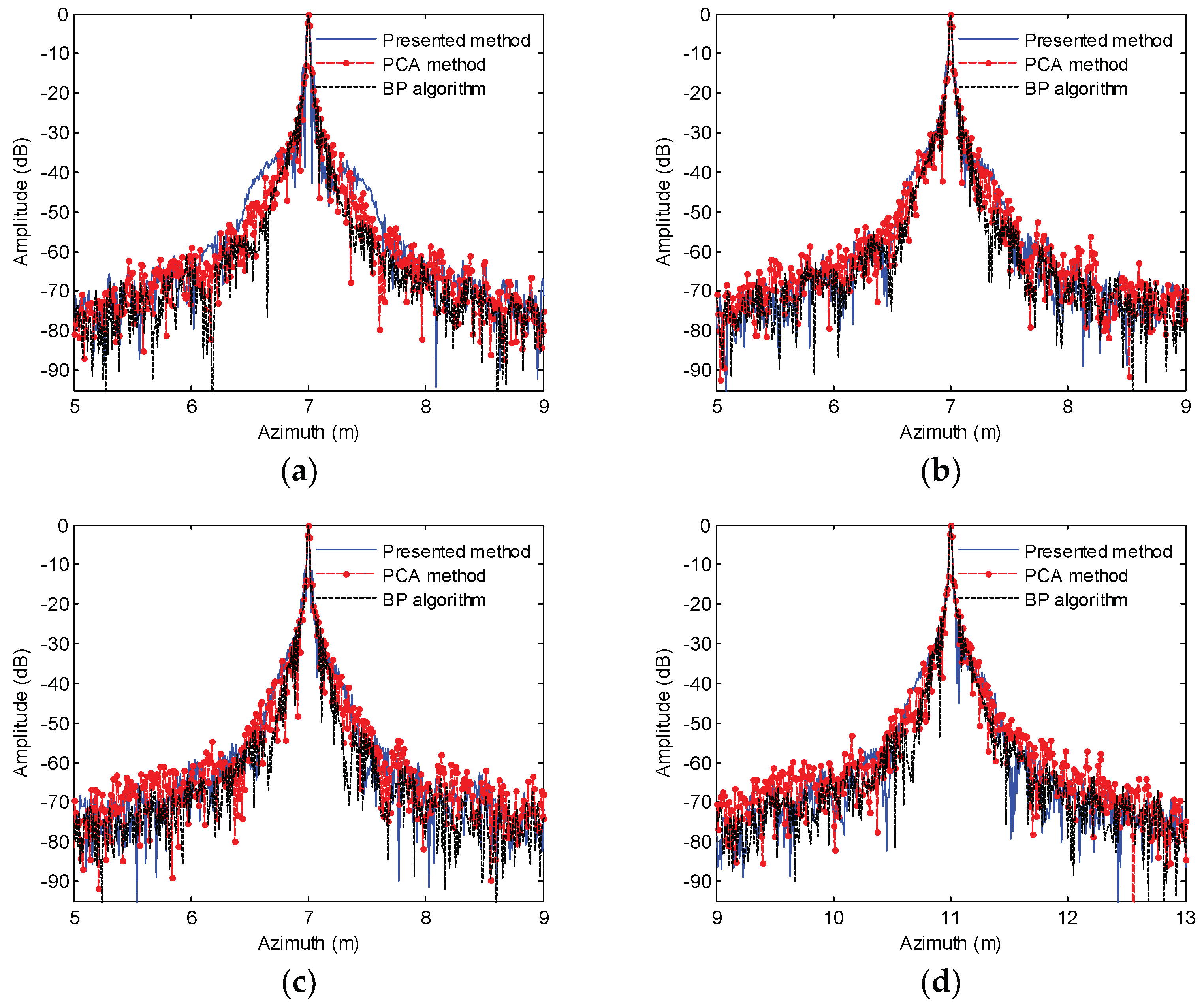
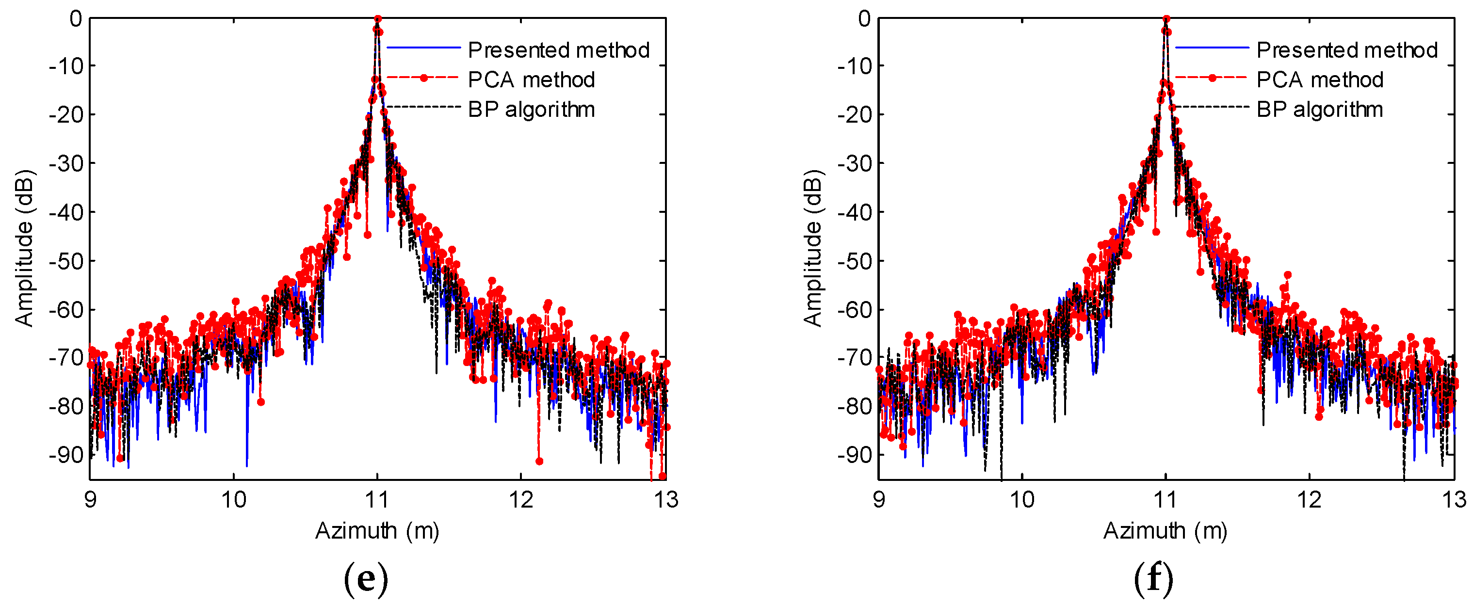
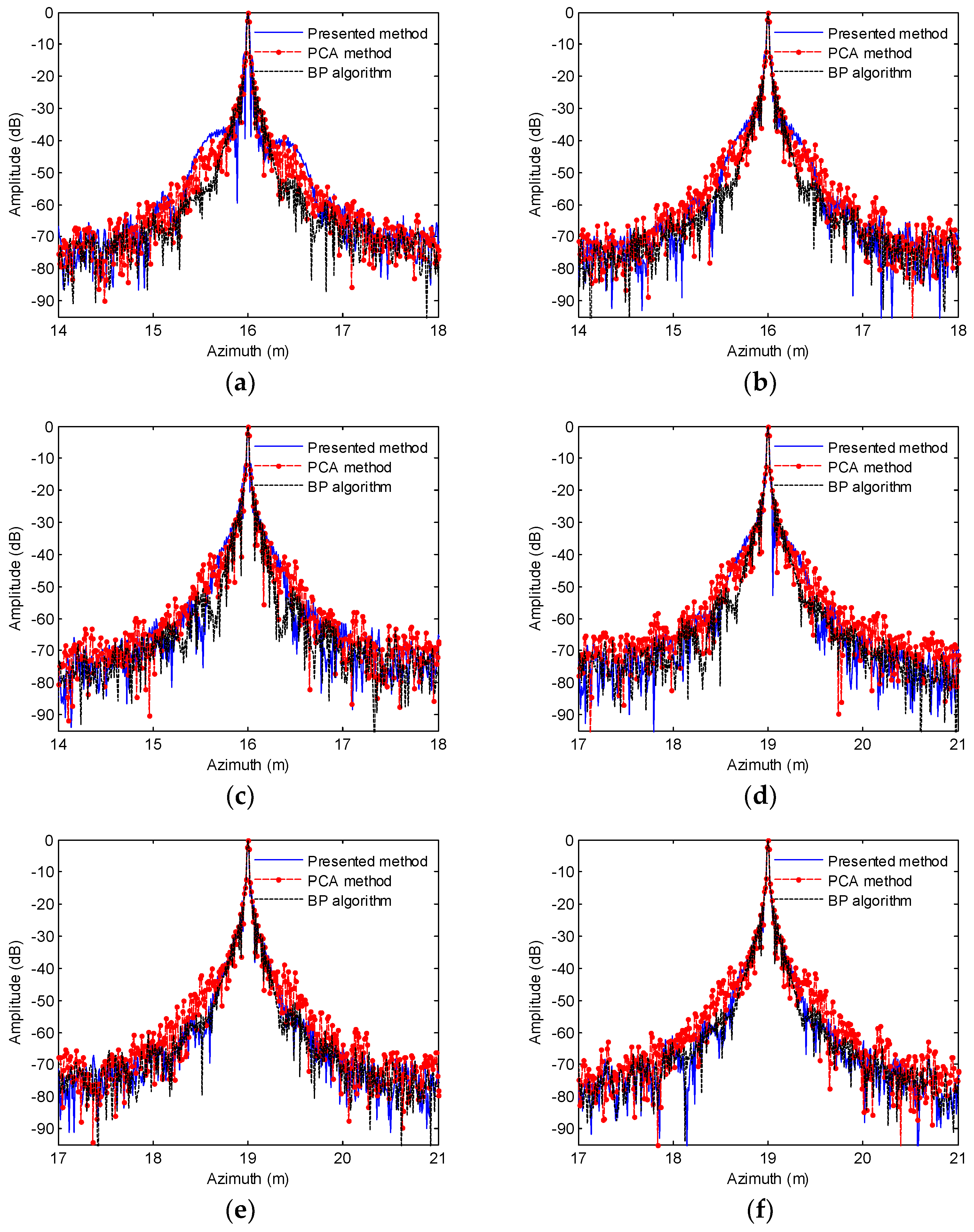
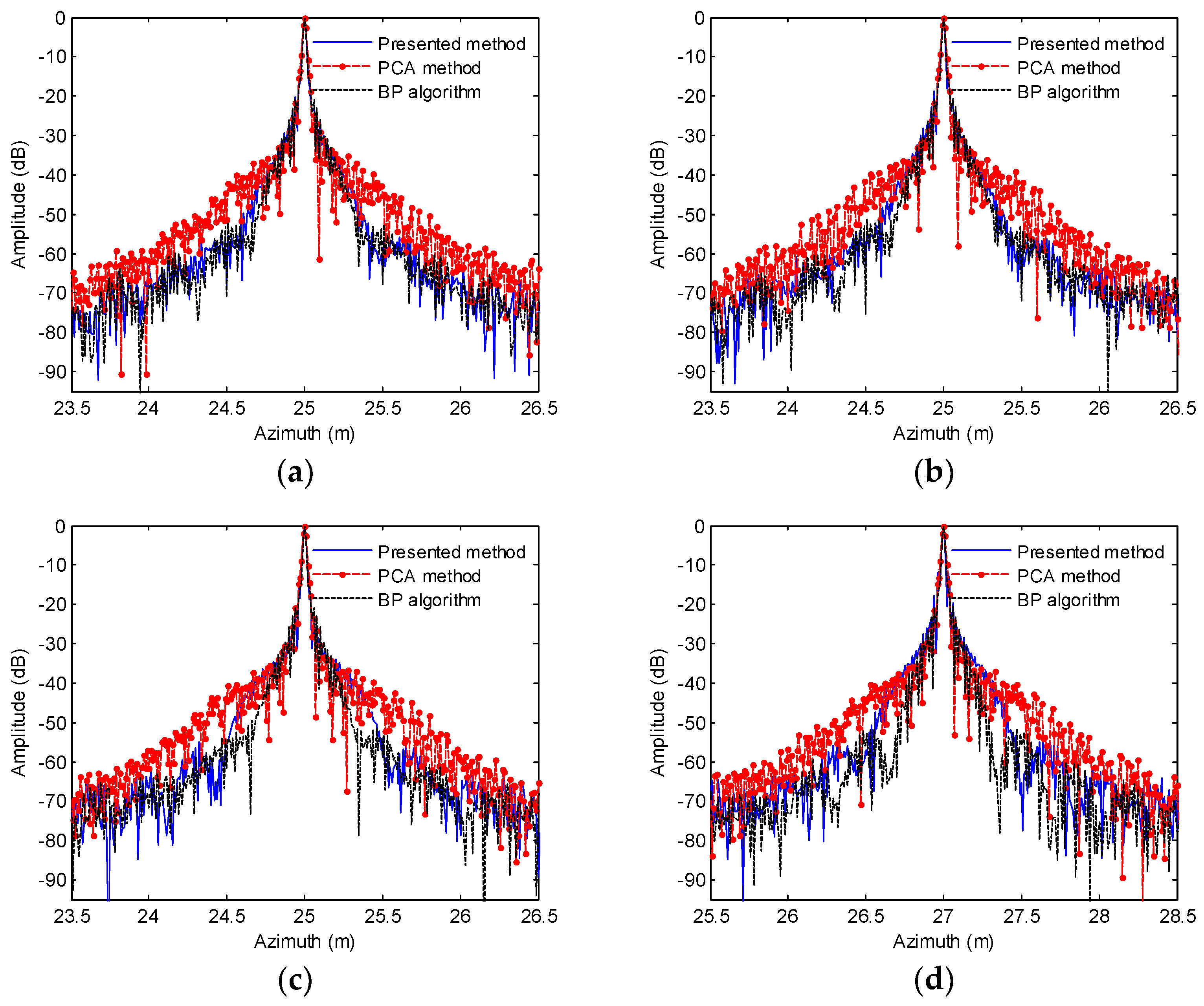
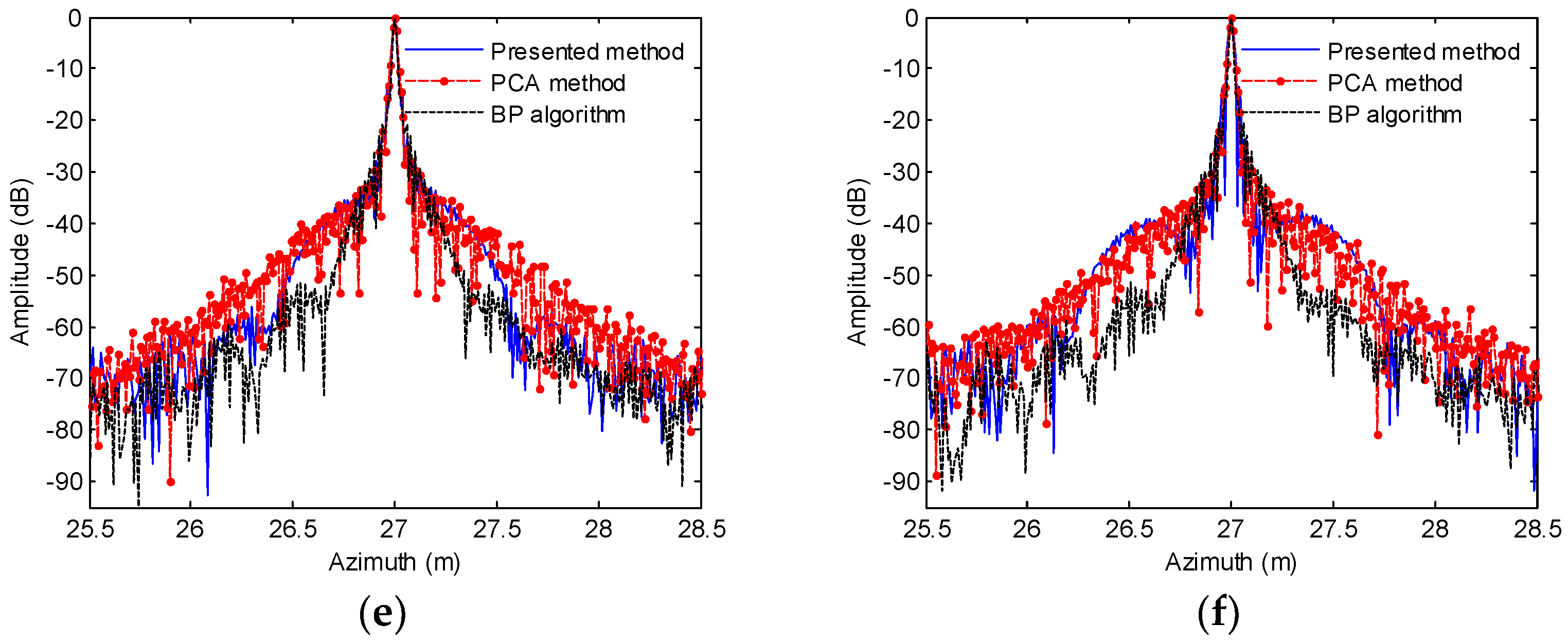
6.1.1. Processing Results of Presented Method

To understand the presented method, the processing results of the main steps are discussed in detail. For clarity, we suppose that there is a point target located at coordinates (141 m, 17 m). Considering the first receiver’s data shown in Figure 4a, we carry out the bulk decoupling in the 2D frequency domain. The resultant signal is shown in Figure 4b. Then, we perform the differential decoupling, and the result is shown in Figure 4c. After this step, the azimuth compression is conducted based on the azimuth modulation. Figure 4d depicts the result after the azimuth compression. Each receiver’s data is undersampled using the pulse repetition frequency, which cannot satisfy the Nyquist rate in azimuth. Due to this reason, all results shown in Figure 4 are aliased in the azimuth dimension. Fortunately, the alias can be suppressed by processing the multireceiver data coherently.
Inspecting Figure 4c,d, we find that both results are visually indistinguishable. In fact, the result shown in Figure 4c is considered to be the input of the subsequent filter, i.e., azimuth compression. Since the azimuth compression performs the phase compensation in the frequency domain, the signal magnitudes are visually indistinguishable in the frequency domain. However, the major difference can be found in the space domain. Applying the azimuth IFT to Figure 4c,d, Figure 5 shows the results in the 2D space domain. From Figure 5b, the signal shown in Figure 5a is compressed in the azimuth dimension, and the circled part represents the recovered target. Each receiver’s data sampled by the pulse repetition frequency is undersampling. Due to this reason, the ghost targets are introduced. The coherent processing of multireceiver data can solve this problem.
Based on the steps in Section 4, M results corresponding to M receiver data are obtained. Each result is similar to Figure 4d. We coherently superpose M results, and the signal is shown in Figure 6a. The coherent superposition is equivalent to the improvement of the sampling rate in azimuth. Therefore, the data shown in Figure 6a satisfies the Nyquist rate, which is increased to M P R F . Performing an azimuth IFT, we obtain the high resolution image, which is shown in Figure 6b. To visually examine the focusing performance, we depict the azimuth slice corresponding to Figure 6b. The azimuth slice is shown in Figure 6c. For comparison, the data shown in Figure 4a is directly processed by the presented method. The azimuth slice corresponding to Figure 5b is also depicted in Figure 6c. From Figure 6c, the azimuth slice related to a single receiver data is aliased, as each receiver data is undersampled by the pulse repetition frequency. By coherently processing multireceiver SAS data, we obtain the high resolution image. Therefore, we conclude that the presented method successfully focuses the point target.

6.1.2. Influence of Sub-Block Width on Imagery

In general, the imaging algorithm can be decomposed into two steps. The first step is to derive the PTRS, coupling term and azimuth modulation. With the presented method, we accurately deduce three terms. The second step is to design the imaging algorithm based on the PTRS, coupling term and azimuth modulation. Since the coupling term in the 2D frequency domain is range variant, we perform the decoupling based on the sub-block processing method. However, it is hard to compensate the coupling term completely. In other words, the sub-block processing method results in the residual error. Here, we discuss the influence of the residual error on the SAS imagery. The imaging scenario consisting of 18-point targets is shown in Figure 7. The targets are marked by T1, T2, …, and T18, respectively. T1, T2, …, and T6 are located at close range. T7, T8, …, and T12 are located at medium range. The remaining targets are supposed to locate at far range. The coupling term is characterized by space variance, which may lead to the space variance of the optimal sub-block width. When the performance of the presented method is not inferior to that of traditional method, the sub-block width used by the presented method is defined as the optimal width of the sub-block. In Figure 7, we depict three sub-blocks, which are denoted by the red, blue and pink rectangles. Each sub-block consists of six targets.
We first focus on the targets circled by the red rectangle in Figure 7. In this sub-block, the reference range used by the differential decoupling is 53 m. The difference between the target range and reference range denotes the half width of the sub-block. The BP algorithm [18] based on (1) is viewed as the precise method. Here, the results of the BP algorithm [22] are used as the criteria. For multireceiver SAS systems, the PCA method [12] is widely used. At this point, we mainly conduct the comparison between the presented method and PCA based R-D algorithm. Figure 8 shows the azimuth slices of T1, …, and T6.
From Figure 8, the performance of the presented method is improved by decreasing the sub-block width. The large width of the sub-block generates great residual error, which noticeably degrades the imaging performance. When the sub-block widths are 14, 12 and 10 m, the performance of the presented method is inferior to that of the PCA method. The performance of the presented method is nearly close to that of the PCA method when the sub-block width is decreased to 8 m. In other words, this sub-block width can satisfy the imagery with high performance at close range. The improvement is still obtained when we choose much narrower sub-block width. However, the improvement is not noticeable. Figure 8f enhances this conclusion.
Next, we use the peak sidelobe level ratio (PSLR) and integral sidelobe level ratio (ISLR) to evaluate the imaging performance. The quality parameters are shown in Table 2.
From Table 2, we see that the presented method obtains a low resolution image with a large sub-block width. The PSLR and ISLR related to T1, T2 and T3 enhances this conclusion. For the target T4, the focusing performance of the presented method is mostly close to that of the PCA method. Considering the target T5, the focusing performance of the presented method is superior to that of the PCA method. In this case, the residual error introduced by the sub-block processing method can be negligible. Inspecting quality parameters of T6, the focusing performance is improved by decreasing the sub-block width. However, the improvement is slight, as the residual error does not dramatically influence the imaging performance. Therefore, we conclude that the sub-block width with 8 m can satisfy the high performance imagery at close range.
We now concentrate on the targets at medium range. In this case, the reference range used for the differential decoupling is 143 m. After the data processing, the azimuth slices are shown in Figure 9.
Inspecting Figure 9, we nearly obtain the same conclusions drawn from Figure 8. When the targets are at medium range, the optimal width of the sub-block is still 8 m. Figure 10b also strengths this conclusion. Since the stop-and-hop error is not completely compensated, the performance of the PCA method is slightly degraded. Based on Figure 8 and Figure 9, the optimal sub-block width of both cases is mostly identical. In other words, the optimal width of the sub-block is nearly range invariant. Table 3 lists quality parameters for targets at medium range.
Based on Table 3, the performance of the presented method is improved with the decreasing of the sub-block width. When the sub-block width is decreased to 8 m, we obtain the image which outperforms that of the PCA method. Due to the residual error of the stop-and-hop approximation, the quality parameters of the PCA method are slightly lowered.
The last experiment focuses on the imaging performance at far range. The reference range used for the differential decoupling in this sub-block is 194 m. The azimuth slices are shown in Figure 10. The residual error of the stop-and-hop assumption increases with the range. Consequently, the PCA method suffers from large residual error when the targets are located at far range. With the presented method, the imaging performance is nearly close to that of the PCA method when the sub-block width is 14 m. Figure 10e enhances this conclusion. By decreasing the sub-block width, the imaging performance of the presented method is improved. From Figure 10b, the sub-block width with 8 m satisfies the high performance imagery. In this case, we obtain the image which is mostly identical to that of the BP algorithm. However, the performance of the PCA method is inferior to that of the presented method and BP algorithm, because the residual error of the stop-and-hop approximation is not completely compensated. Inspecting Figure 8 and Figure 9, the optimal sub-block width is about 8 m for three cases. In practice, the large sub-block width can be used at far range without loss of the imaging performance.
For targets at far range, the PSLR and ISLR are listed in Table 4. When the sub-block width is large, the error introduced by the sub-block processing method noticeably degrades the imaging performance of the presented method. The focusing performance of T15, T16, T17 and T18 also enhances this conclusion. The result of the presented method can be improved by decreasing the sub-block width. With the presented method, we obtain the high resolution results when the sub-block width is less than 8 m. The PSLR and ISLR related to T13 and T14 further strength this conclusion. However, the performance of the PCA method is greatly affected by the residual error of the stop-and-hop approximation at far range.
Since the coupling term is space variant, the sub-block processing method is exploited to perform the decoupling operation. However, the sub-block method introduces the residual phase error, which is expressed as | φ d e _ i ( f τ , f t ; r ref _ n ± Δ r / 2 ) φ d e _ i ( f τ , f t ; r ref _ n ) | . Here, Δ r denotes the sub-block width. Generally speaking, the imaging performance of the presented method highly depends on the sub-block width. In each sub-block, the residual phase error introduced by the decoupling operation should be limited within π / 4 [31]. Under this condition, the influence of the phase error can be neglected.
Figure 8a, Figure 9a and Figure 10f are based on the sub-block width with 20 m. We find that the slices of the presented method are inferior to the slices of the PCA algorithm and BP method. The reason behind this is that the residual coupling error is not completely compensated. Hence, there is still the coupling between the range and azimuth dimensions. T1, T7 and T18 are far away from the sub-block center. The corresponding sub-blocks have a large width. Based on the decoupling phase of reference targets at the sub-block center, the decoupling operation across the whole sub-block is carried out. When the targets are at the sub-block edge, this operation introduces large residual coupling error, which is not limited within π / 4 . Due to this reason, the azimuth focusing performance such as the azimuth slice, PSLR and ISLR is seriously degraded. The focusing results of T1, T7 and T18 enhance this conclusion. When the targets are close to the sub-block center, the residual coupling error does not noticeably affect the SAS focusing performance. Under this condition, the residual coupling error limited within π / 4 can be negligible. Considering the trade-off between the imaging efficiency and performance, the optimal width of the sub-block is often exploited. In this case, the imaging performance of the presented method is nearly close to that of the BP method. The processing results of T5, T11 and T14 enhance this conclusion. Generally, the presented method can obtain the high resolution image across the whole swath based on the optimal width of the sub-block. Besides, it is very suitable for the SAS imagery with wide swath.

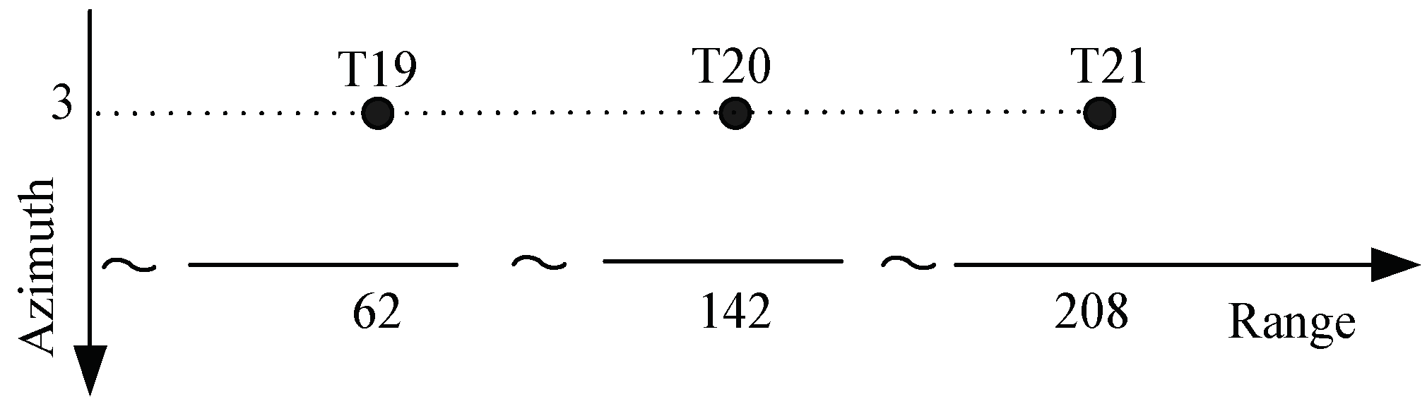
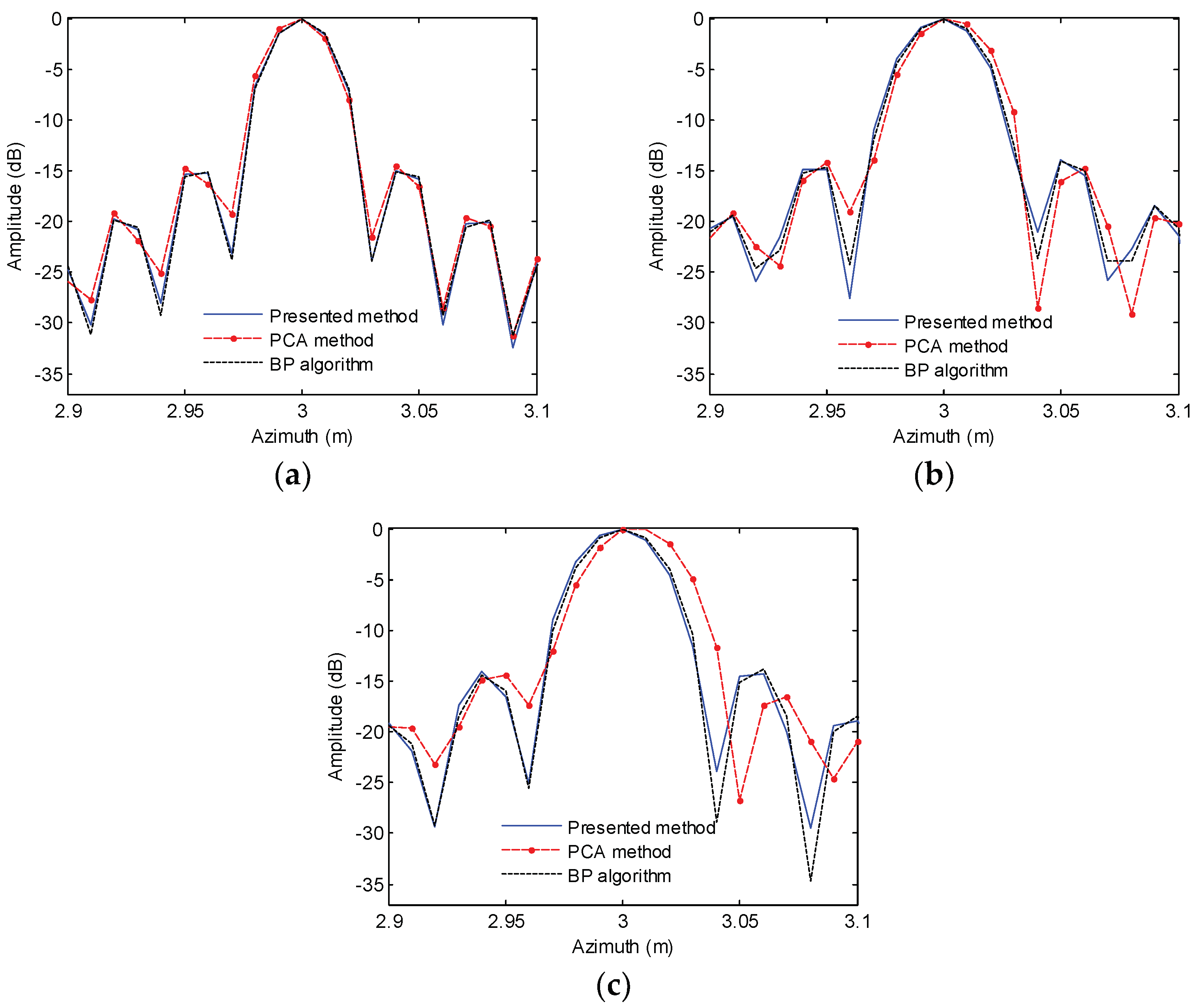
6.1.3. Imaging Performance at Scenario Edge

Since the error of the stop-and-hop approximation is space variant, it is difficult to compensate this error using traditional methods. Fortunately, the presented method successfully solves this problem based on the accurate time delay of the signal. We now concentrate on the focusing performance at the scenario edge. Figure 11 shows the imaging scenario including three ideal targets.
Based on the presented method, the PCA method and BP algorithm, the azimuth slices of focused targets are shown in Figure 12.
With the presented method and PCA method, the target coordinates in Figure 12a are mostly accordant with coordinates shown in Figure 11. Considering the PCA method, there is a slight deviation of the azimuth coordinate in Figure 12b. Generally, this deviation can be negligible at close range. Inspecting Figure 12c, the PCA method suffers from noticeable deviation of the azimuth coordinate, and the deviation is about 0.01 m. Since the PCA method does not completely compensate the error of the stop-and-hop approximation, the residual error is introduced. It increases with the range and slow time. Due to this reason, the deviation can be negligible at close range. However, the deviation leads to the distortion when there are distributed targets at far range. Using the presented method, the targets across the whole swath are well focused.

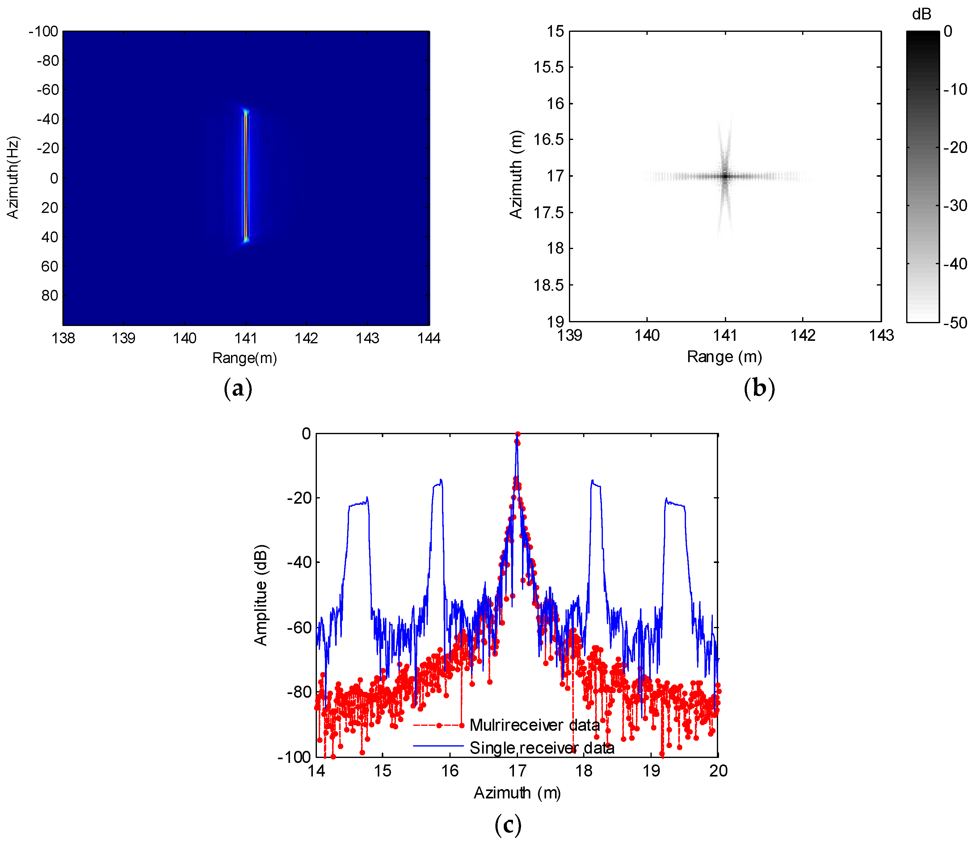
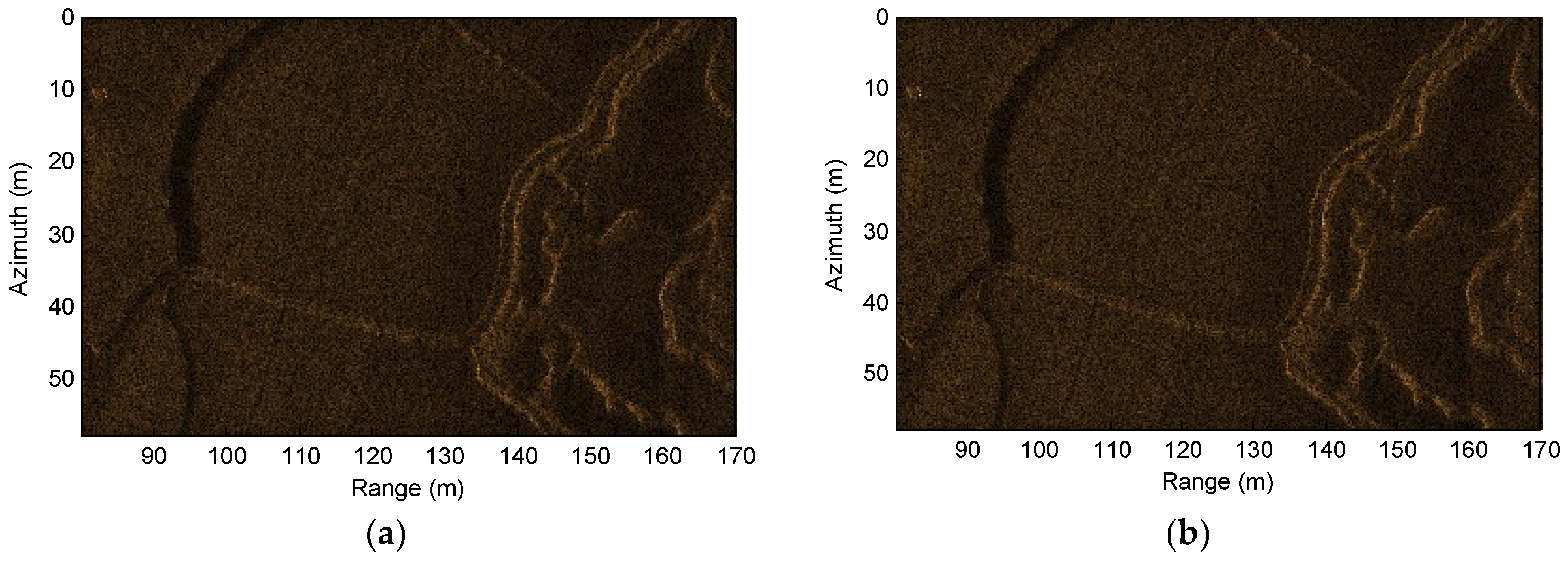
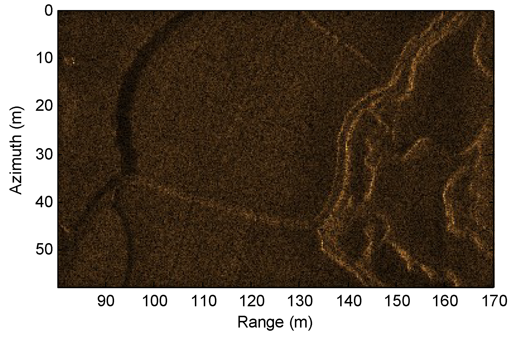
6.2. Real Data Processing

We tested the presented method based on the real data. The data has 4800 sampling points in the range dimension and 3200 spatial sampling points in the azimuth dimension. For the transmitted signal, the center frequency and bandwidth are 150 kHz and 20 kHz, respectively. The receiver array, including 40 uniformly spaced receivers, is 1.6 m in azimuth. The velocity of the sonar platform is 2.5 m/s. When it comes to the operation of the differential decoupling with the presented method, two cases including four sub-blocks and eight sub-blocks in the range dimension are considered. The corresponding results are shown in Figure 13a,b, respectively. From Figure 13, it can be seen that the processing results of both cases are mostly identical. Therefore, we can draw a conclusion that the requirement of the sub-block segmentation in the range dimension can be relaxed. In practice, we can use large sub-block width without loss of performance when the real data is processed based on the presented method. For comparison, the real data is still processed by the BP algorithm. Figure 14 shows the processing result of the BP algorithm. Inspecting Figure 13 and Figure 14, the presented method provide the high resolution result, which is mostly identical to that of the BP algorithm.
The processing time with both methods are listed in Table 5.
Both algorithms are developed based on Matlab 2012a. The processing time of the BP algorithm based on the sinc interpolation is 35,234 s. There are two schemes to develop the program of the presented method. With the first scheme, the calculation of the PSP and azimuth PSP are integrated with the imaging algorithm. It is time consuming due to the numerical evaluation of PSPs. In practice, the numerical calculation of PSPs can be carried out ahead of the focusing. With stored PSPs, we run the imaging algorithm. This is the second scheme. With this scheme, the processing time with four sub-blocks is decreased to 608 s. With the second scheme, the efficiency is dramatically improved compared with the first scheme. At this point, the second scheme is used with the real data processing. From Table 5, the presented algorithm with eight sub-blocks costs 1149 s. Overall, the processing time of the presented method increases with sub-blocks in range, because more time is needed to perform the differential decoupling. In comparison with the BP algorithm, the efficiency of presented method has been improved 30.7 times at least. Nowadays, the parallel algorithm and tools such as graphics processing unit (GPU), faster Fourier transform in the west (FFTW) and intel@ math kernel library (MKL) can be used to improve the efficiency of the presented method dramatically. Our future work is to optimize our method using parallel algorithms.

7. Conclusions

In this paper, we present a novel imaging algorithm for the multireceiver SAS based on the accurate time delay and numerical evaluation method. The presented method first deduces the PTRS and azimuth modulation using the numerical evaluation method. Then the difference between the PTRS and azimuth modulation denotes the coupling term. The key issue of the SAS imagery is the decoupling operation, which consists of two parts: the bulk and differential decoupling. The bulk decoupling mainly deals with the spatial invariance of the coupling term. Considering targets at reference range, the coupling is completely removed after this step. However, other targets suffer from the residual coupling error. The differential decoupling is carried out to solve this problem. Considering the spatial variance of the residual coupling error, the sub-block processing in range is exploited.
Based on the simulations, the focusing performance of the traditional method is greatly degraded at far range, as the residual error introduced by the stop-and-hop approximation increases with the range. Using the optimal width of the sub-block, the presented method achieves high performance results compared with traditional method.

Author Contributions

X.Z. and W.Y. carried out all of the analysis and algorithms and wrote the paper. C.T. designed part of experiments. All authors read and approved the final manuscript.

Funding

This research was funded by the National Natural Science Foundation of China (61601473) and National Key Laboratory Foundation (9140C290401150C29132).

Acknowledgments

The authors would like to thank the anonymous reviewers and editors for their constructive comments and suggestions. Wei Chen offered advice on the language and revision.

Conflicts of Interest

The authors declare no conflict of interest.

References

  1. Williams, D.P. The Mondrian detection algorithm for sonar imagery. IEEE Trans. Geosci. Remote Sens. 2018, 56, 1091–1102. [Google Scholar] [CrossRef]
  2. Larsen, L.J.; Wilby, A.; Stewart, C. Deepwater ocean survey and search using synthetic aperture sonar. In Proceedings of the 2010 MTS/IEEE Oceans Conference, Seattle, WA, USA, 20–23 September 2010; pp. 1–4. [Google Scholar]
  3. LeHardy, P.K.; Larsen, L.J. Deepwater synthetic aperture sonar and the search for MH 370. In Proceedings of the 2015 MTS/IEEE Oceans Conference, Washington, DC, USA, 19–22 October 2015; pp. 1–4. [Google Scholar]
  4. Odegard, O.; Ludvigsen, M.; Lagstad, A. Using synthetic aperture sonar in marine archaeological surveys—Some first experiences. In Proceedings of the 2013 MTS/IEEE Oceans Conference, Bergen, Norway, 10–14 June 2013; pp. 1–7. [Google Scholar]
  5. Carballini, J.; Viana, F. Using synthetic aperture sonar as an effective tool for pipeline inspection survey projects. In Proceedings of the 2015 MTS/OES RIO Acoustics, Rio de Janeiro, Brazil, 29–31 July 2015; pp. 1–5. [Google Scholar]
  6. Groen, J.; Coiras, E.; Vera, J.D.R.; Evans, B. Model-based sea mine classification with synthetic aperture sonar. IET Radar Sonar Navig. 2010, 4, 62–73. [Google Scholar] [CrossRef]
  7. Wu, H.; Tang, J.; Zhong, H. A correction approach for the inclined array of hydrophones in synthetic aperture sonar. Sensors 2018, 18, 2000. [Google Scholar] [CrossRef] [PubMed]
  8. Tang, S.; Guo, P.; Zhang, L.; Lin, C. Modeling and precise processing for spaceborne transmitter/missile-borne receiver SAR signals. Remote Sens. 2019, 11, 346. [Google Scholar] [CrossRef]
  9. Cumming, I.G.; Wong, F.H. Digital Processing of Synthetic Aperture Radar Data: Algorithms and Implementation; Artech House: Norwood, MA, USA, 2005. [Google Scholar]
  10. Wilkinson, D.R. Efficient Image Reconstruction Techniques for a Multiple-Receiver Synthetic Aperture Sonar. Master’s Thesis, Department of Electrical and Computer Engineering, University of Canterbury, Christchurch, New Zealand, July 1999. [Google Scholar]
  11. Bonifant, W.W. Interferometric Synthetic Aperture Sonar Processing. Master’s Thesis, Georgia Institute of Technology, Atlanta, GA, USA, July 1999. [Google Scholar]
  12. Zhang, X.; Tang, J.; Zhong, H. Multireceiver correction for the chirp scaling algorithm in synthetic aperture sonar. IEEE J. Ocean. Eng. 2014, 39, 472–481. [Google Scholar] [CrossRef]
  13. Gough, P.T.; Hayes, M.P. Fast Fourier techniques for SAS imagery. In Proceedings of the 2005 MTS/IEEE Oceans Conference, Brest, France, 20–23 June 2005; pp. 563–568. [Google Scholar]
  14. Loffeld, O.; Nies, H.; Peters, V.; Knedlik, S. Models and useful relations for bistatic SAR processing. IEEE Trans. Geosci. Remote Sens. 2004, 42, 2031–2038. [Google Scholar] [CrossRef] [Green Version]
  15. Zhang, X.; Yang, P. Imaging algorithm for multireceiver synthetic aperture sonar. J. Electr. Eng. Technol. 2019, 14, 471–478. [Google Scholar] [CrossRef]
  16. Yang, H.; Tang, J.; Chen, M.; Chen, X. A multiple-receiver synthetic aperture sonar wavenumber imaging algorithm with non-uniform sampling in azimuth. J. Wuhan Univ. Technol. (Transp. Sci. Eng.) 2011, 35, 993–996. [Google Scholar]
  17. Zhang, X.; Chen, X.; Qu, W. Influence of the stop-and-hop assumption on synthetic aperture sonar imagery. In Proceedings of the 2017 International Conference on Communication Technology, Chengdu, China, 27–30 October 2017; pp. 1601–1607. [Google Scholar]
  18. Wang, G.; Zhang, L.; Li, J.; Hu, Q. Precise aperture-dependent motion compensation for high-resolution synthetic aperture radar imaging. IET Radar Sonar Navig. 2017, 11, 204–211. [Google Scholar] [CrossRef]
  19. Zhang, X.; Tang, J.; Zhang, S.; Bai, S.; Zhong, H. Four order polynomial based range-Doppler algorithm for multireceiver synthetic aperture sonar. J. Electron. Inf. Technol. 2014, 36, 1592–1598. [Google Scholar]
  20. Wu, Q.; Xing, M.; Shi, H.; Hu, X.; Bao, Z. Exact analytical two-dimensional spectrum for bistatic synthetic aperture radar in tandem configuration. IET Radar Sonar Navig. 2011, 5, 349–360. [Google Scholar] [CrossRef]
  21. Tian, Z.; Tang, J.; Zhong, H.; Zhang, S. Extended range Doppler algorithm for multiple-receiver synthetic aperture sonar based on exact analytical two-dimensional spectrum. IEEE J. Ocean. Eng. 2016, 41, 3350–3358. [Google Scholar]
  22. Xu, J.; Tang, J.; Zhang, C. Multi-aperture synthetic aperture sonar imaging algorithm. Signal Process. 2003, 19, 157–160. [Google Scholar]
  23. Wu, J.; Xu, Y.; Zhong, X.; Sun, Z.; Yang, J. A three-dimensional localization method for multistatic SAR based on numerical range-Doppler algorithm and entropy minimization. Remote Sens. 2017, 9, 470. [Google Scholar] [CrossRef]
  24. Jin, M.Y.; Wu, C. A SAR correlation algorithm which accommodates large-range migration. IEEE Trans. Geosci. Remote Sens. 1984, GE-22, 592–597. [Google Scholar] [CrossRef]
  25. Chen, P.; Kang, J. Improved chirp scaling algorithms for SAR imaging under high squint angles. IET Radar Sonar Navig. 2017, 11, 1629–1636. [Google Scholar] [CrossRef]
  26. Wong, F.H.; Yeo, T.S. New applications of nonlinear chirp scaling in SAR data processing. IEEE Trans. Geosci. Remote Sens. 2001, 39, 946–953. [Google Scholar] [CrossRef]
  27. Li, Y.; Huang, P.; Lin, C. Focus improvement of highly squint bistatic synthetic aperture radar based on non-linear chirp scaling. IET Radar Sonar Navig. 2017, 11, 171–176. [Google Scholar] [CrossRef]
  28. Wang, K.; Liu, X. Quartic-phase algorithm for highly squinted SAR data processing. IEEE Geosci. Remote Sens. Lett. 2007, 4, 246–250. [Google Scholar] [CrossRef]
  29. Guo, P.; Tang, S.; Zhang, L.; Sun, G. Improved focusing approach for highly squinted beam steering SAR. IET Radar Sonar Navig. 2016, 10, 1394–1399. [Google Scholar] [CrossRef]
  30. Ku, C.S.; Chen, K.S.; Chang, P.C.; Chang, Y.L. Imaging simulation for synthetic aperture radar: A full-wave approach. Remote Sens. 2018, 10, 1404. [Google Scholar] [CrossRef]
  31. Wu, J.; An, H.; Zhang, Q.; Sun, Z.; Li, Z.; Du, K.; Huang, Y.; Yang, J. Two-dimensional frequency decoupling method for curved trajectory synthetic aperture radar imaging. IET Radar Sonar Navig. 2018, 12, 766–773. [Google Scholar] [CrossRef]
Figure 1. Imaging geometry of the multireceiver synthetic aperture sonar (SAS).
Remotesensing 11 00672 g001
Figure 2. Block diagram of the presented processor. See the text (sections: PTRS, azimuth modulation and coupling term, and imaging algorithm) for all terms and full names of abbreviations used in the figure.
Remotesensing 11 00672 g002
Figure 3. Deduction of three important functions. (a) Presented method; (b) traditional methods. See the text (section: Introduction) for all terms and full names of abbreviations used in the figure.
Remotesensing 11 00672 g003
Figure 4. Processing results of a single receiver data. (a) Single receiver data; (b) bulk decoupling; (c) differential decoupling; (d) azimuth compression.
Remotesensing 11 00672 g004
Figure 5. Results in the two-dimensional (2D) space domain. (a) Differential decoupling; (b) azimuth compression.
Remotesensing 11 00672 g005
Figure 6. Processing results of all receiver data. (a) Coherent superposition; (b) focused target; (c) azimuth slice.
Remotesensing 11 00672 g006
Figure 7. Simulated scenario with 18-point targets.
Remotesensing 11 00672 g007
Figure 8. Azimuth slices of close targets. (a) Sub-block width with 20 m; (b) sub-block width with 14 m; (c) sub-block width with 12 m; (d) sub-block width with 10 m; (e) sub-block width with 8 m; and (f) sub-block width with 2 m.
Remotesensing 11 00672 g008aRemotesensing 11 00672 g008b
Figure 9. Azimuth slices of medium range targets. (a) Sub-block width with 20 m; (b) sub-block width with 14 m; (c) sub-block width with 12 m; (d) sub-block width with 10 m; (e) sub-block width with 8 m; and (f) sub-block width with 2 m.
Remotesensing 11 00672 g009
Figure 10. Azimuth slices of far targets. (a) Sub-block width with 2 m; (b) sub-block width with 8 m; (c) sub-block width with 10 m; (d) sub-block width with 12 m; (e) sub-block width with 14 m; and (f) sub-block width with 20 m.
Remotesensing 11 00672 g010aRemotesensing 11 00672 g010b
Figure 11. Simulated scenario with three-point targets.
Remotesensing 11 00672 g011
Figure 12. Azimuth slices of T19, T20 and T21. (a) T19; (b) T20; (c) T21.
Remotesensing 11 00672 g012
Figure 13. Processing results of the presented method. (a) Four sub-blocks; (b) eight sub-blocks.
Remotesensing 11 00672 g013
Figure 14. Processing results of the BP algorithm.
Remotesensing 11 00672 g014
Table 1. The SAS System Parameters.
ParametersValueUnits
Center frequency150kHz
Bandwidth20kHz
Platform velocity2m/s
Receiver length in azimuth0.02m
Length of receiver array0.6m
Transmitter length in azimuth0.04m
Pulse repetition interval0.3s
Table 2. Quality parameters for targets at close range. PCA: phase center approximation; BP: back projection; PSLR: peak sidelobe level ratio; ISLR: integral sidelobe level ratio.
Presented MethodPCA MethodBP Method
PSLR/dBISLR/dBPSLR/dBISLR/dBPSLR/dBISLR/dB
T1−11.61−6.44−14.38−9.57−14.83−10.34
T2−13.01−8.36−14.45−9.49−14.88−10.25
T3−10.82−8.21−14.54−9.98−14.90−10.82
T4−13.41−9.39−14.63−9.68−14.77−10.44
T5−14.61−9.87−14.44−9.59−14.81−10.15
T6−14.69−10.12−14.26−9.60−14.69−10.06
Table 3. Quality parameters for targets at medium range.
Presented MethodPCA MethodBP Method
PSLR/dBISLR/dBPSLR/dBISLR/dBPSLR/dBISLR/dB
T7−11.61−6.44−13.92−9.52−14.81−10.23
T8−13.26−8.67−13.87−9.37−14.92−10.25
T9−10.36−7.87−13.86−9.32−14.77−10.09
T10−13.86−9.38−14.01−9.71−14.78−10.28
T11−14.02−9.53−13.73−9.22−14.87−10.21
T12−14.13−10.13−13.69−9.17−14.7−10.12
Table 4. Quality parameters for targets at far range.
Presented MethodPCA MethodBP Method
PSLR/dBISLR/dBPSLR/dBISLR/dBPSLR/dBISLR/dB
T13−14.49−10.22−13.23−9.93−14.76−10.26
T14−14.17−9.97−13.13−9.8−14.80−10.22
T15−13.23−9.60−12.87−9.47−14.72−10.35
T16−12.45−7.83−12.99−9.39−14.83−10.18
T17−11.96−8.80−13.15−9.79−14.86−10.41
T18−11.28−6.51−13.55−9.67−14.78−10.21
Table 5. Processing time of imaging methods.
Presented MethodBP Algorithm
Four Sub-BlocksEight Sub-Blocks
Processing time/s608114935234

