Operational Large-Scale Segmentation of Imagery Based on Iterative Elimination


Abstract
:
1. Introduction
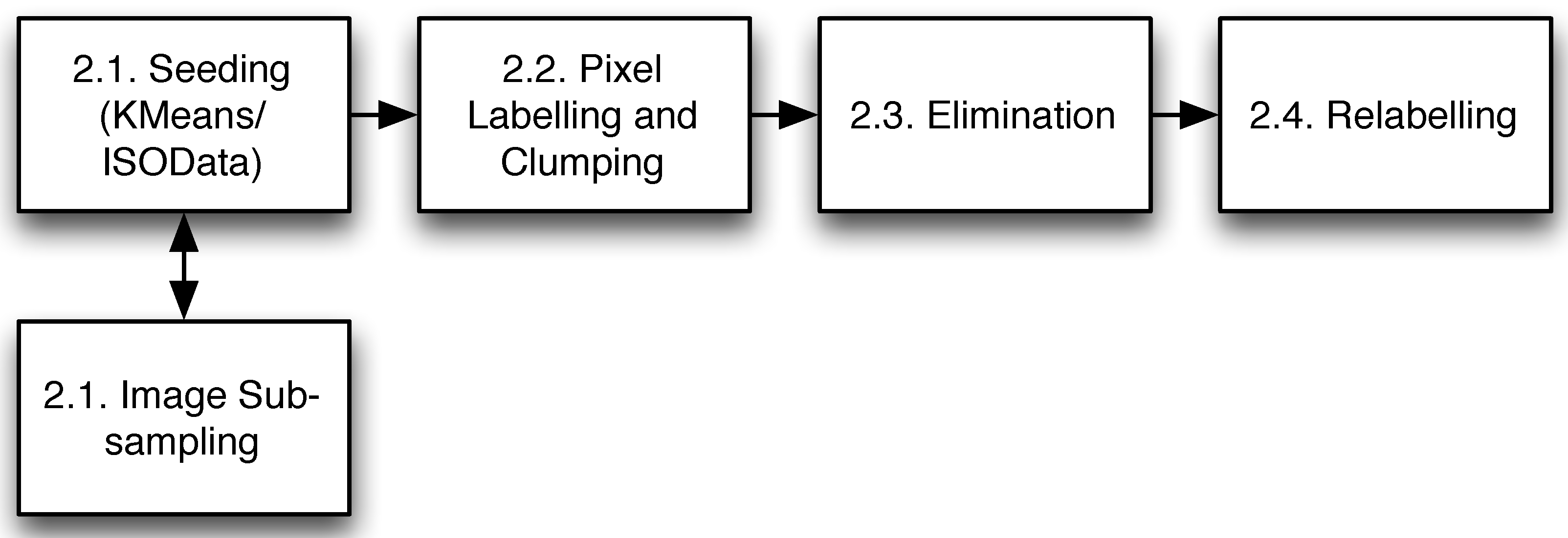
2. Methods
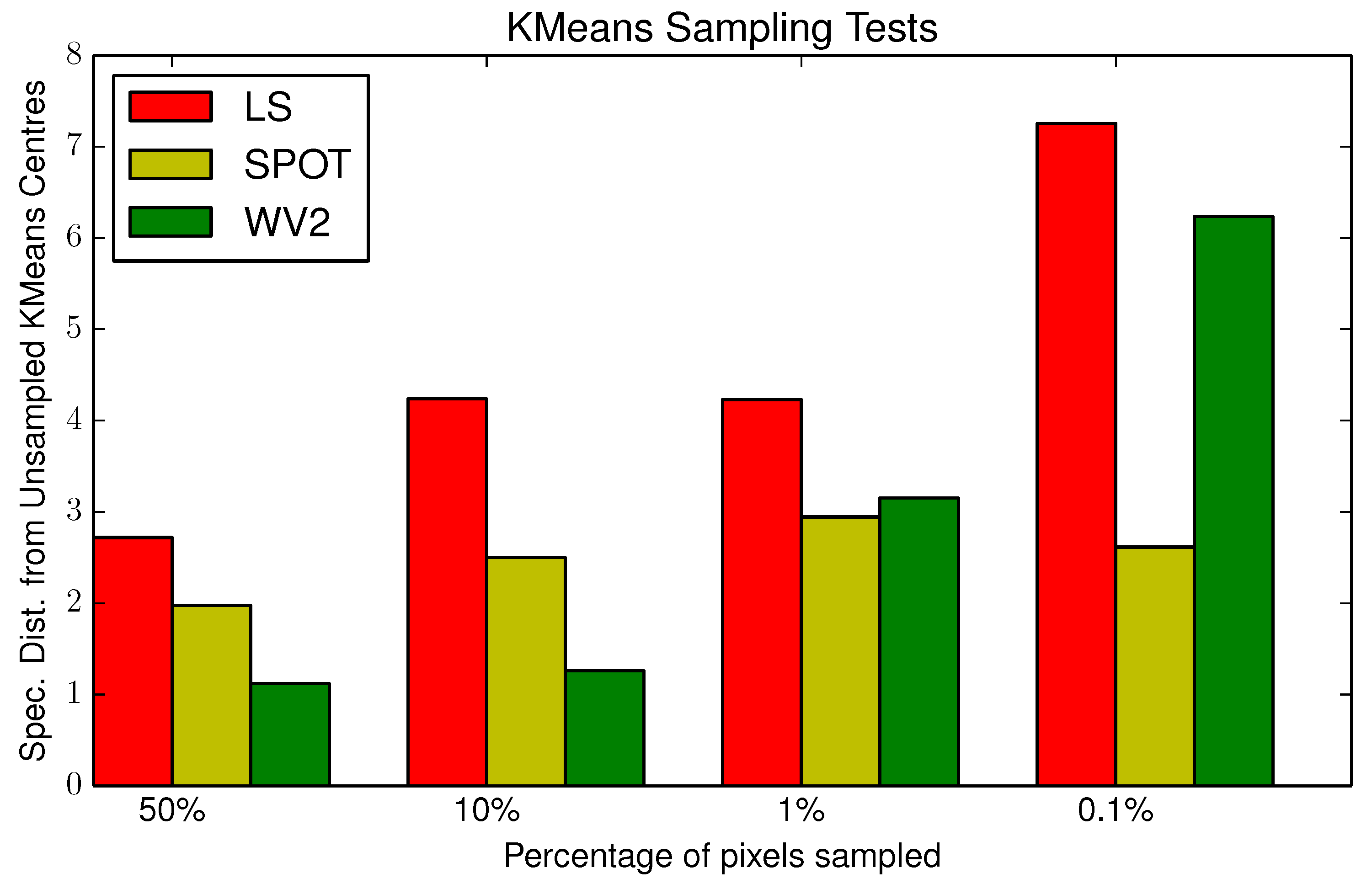
2.1. Seeding
2.2. Clumping
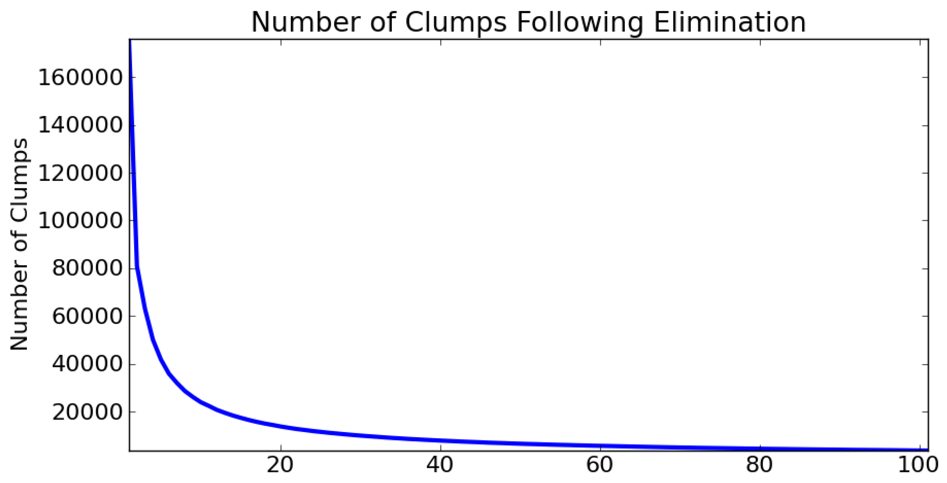
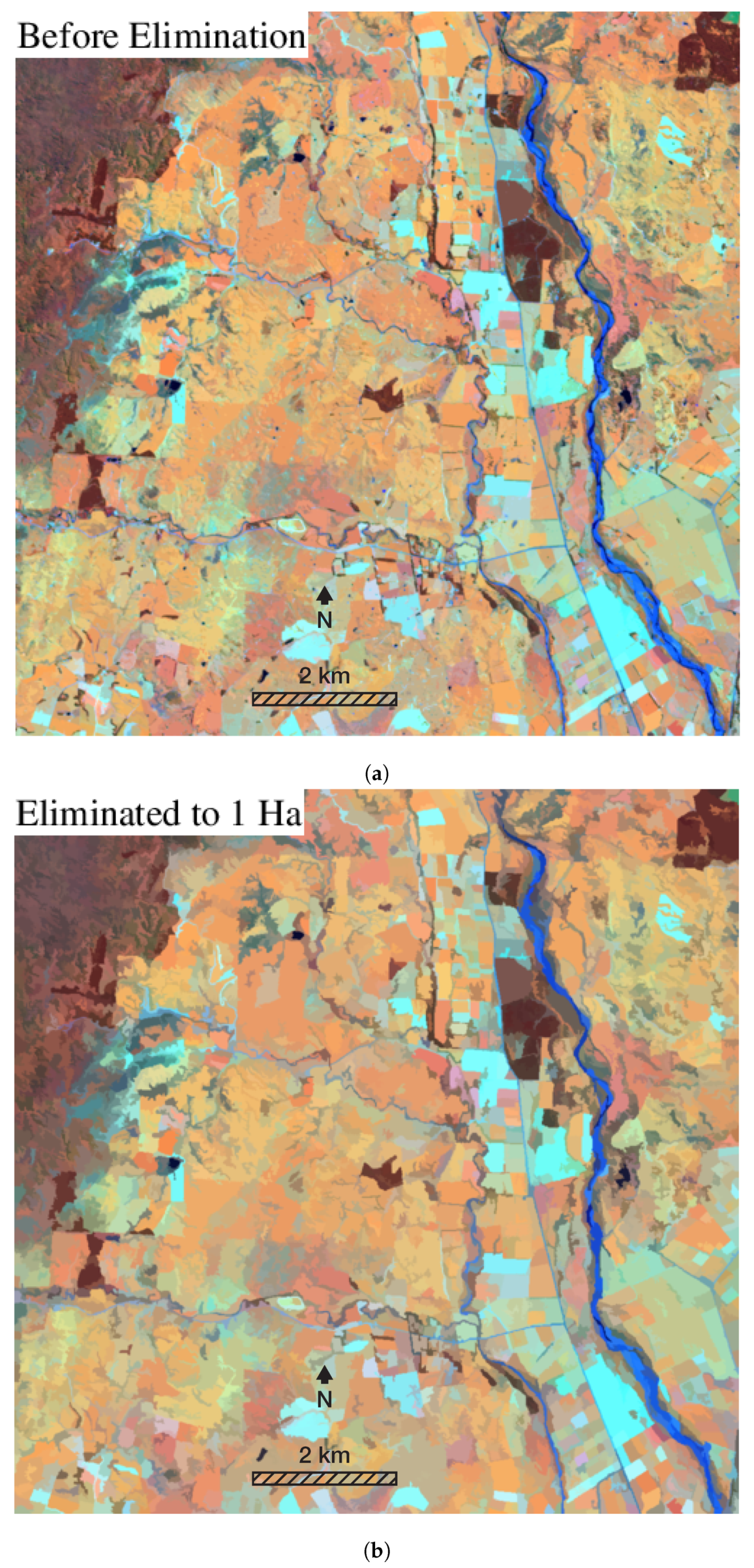
2.3. Local Elimination
| Algorithm 1 Pseudocode for the elimination process. |
|
2.4. Relabelling
2.5. Parameterisation
3. Results
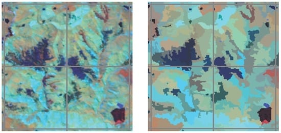
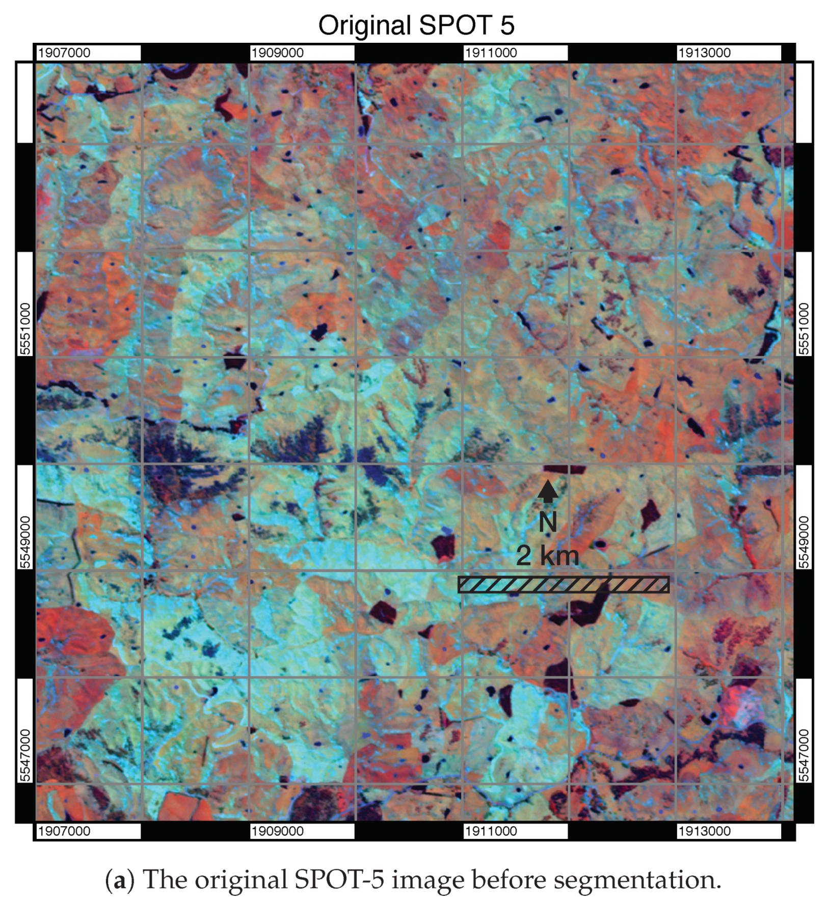
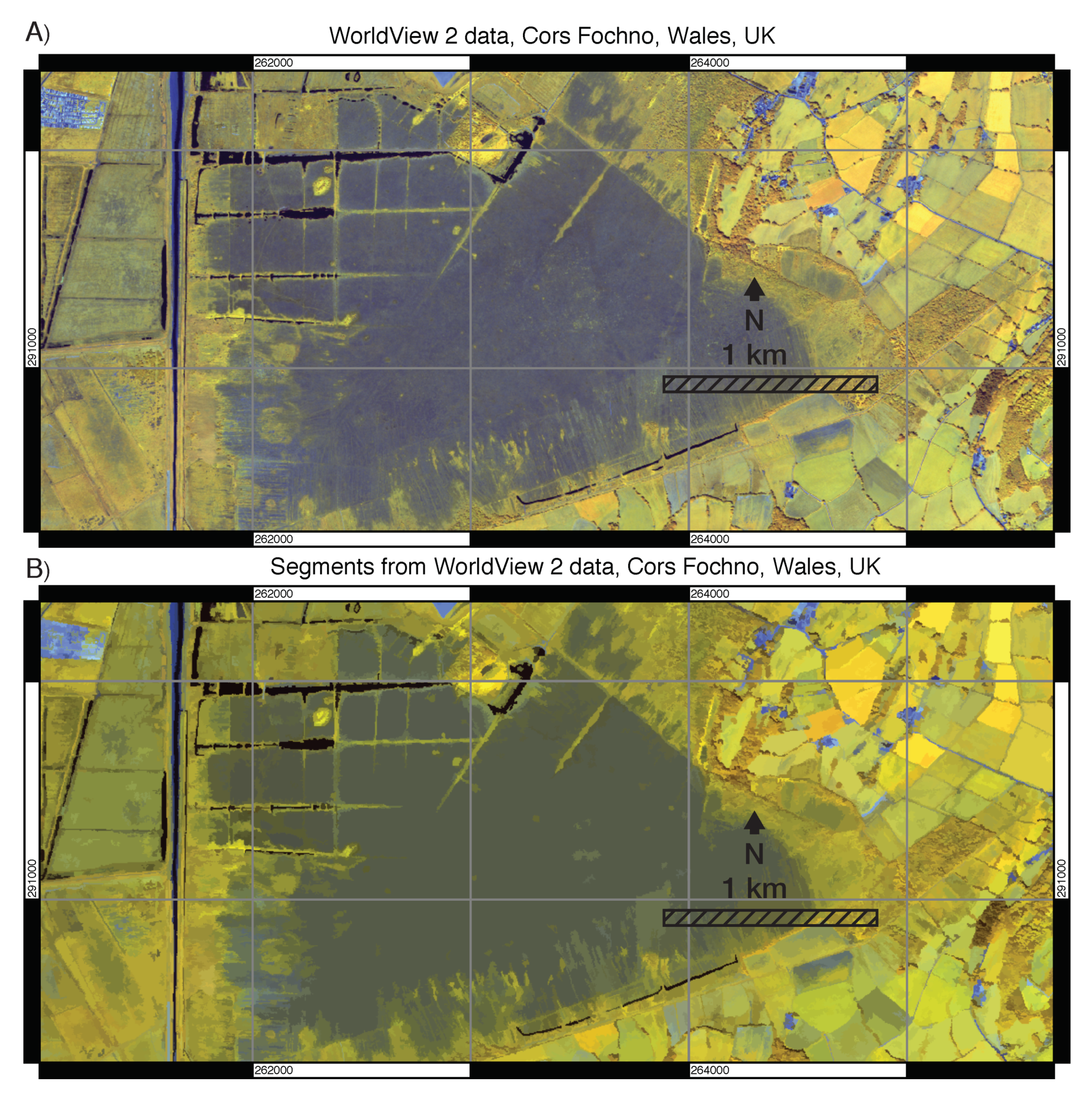
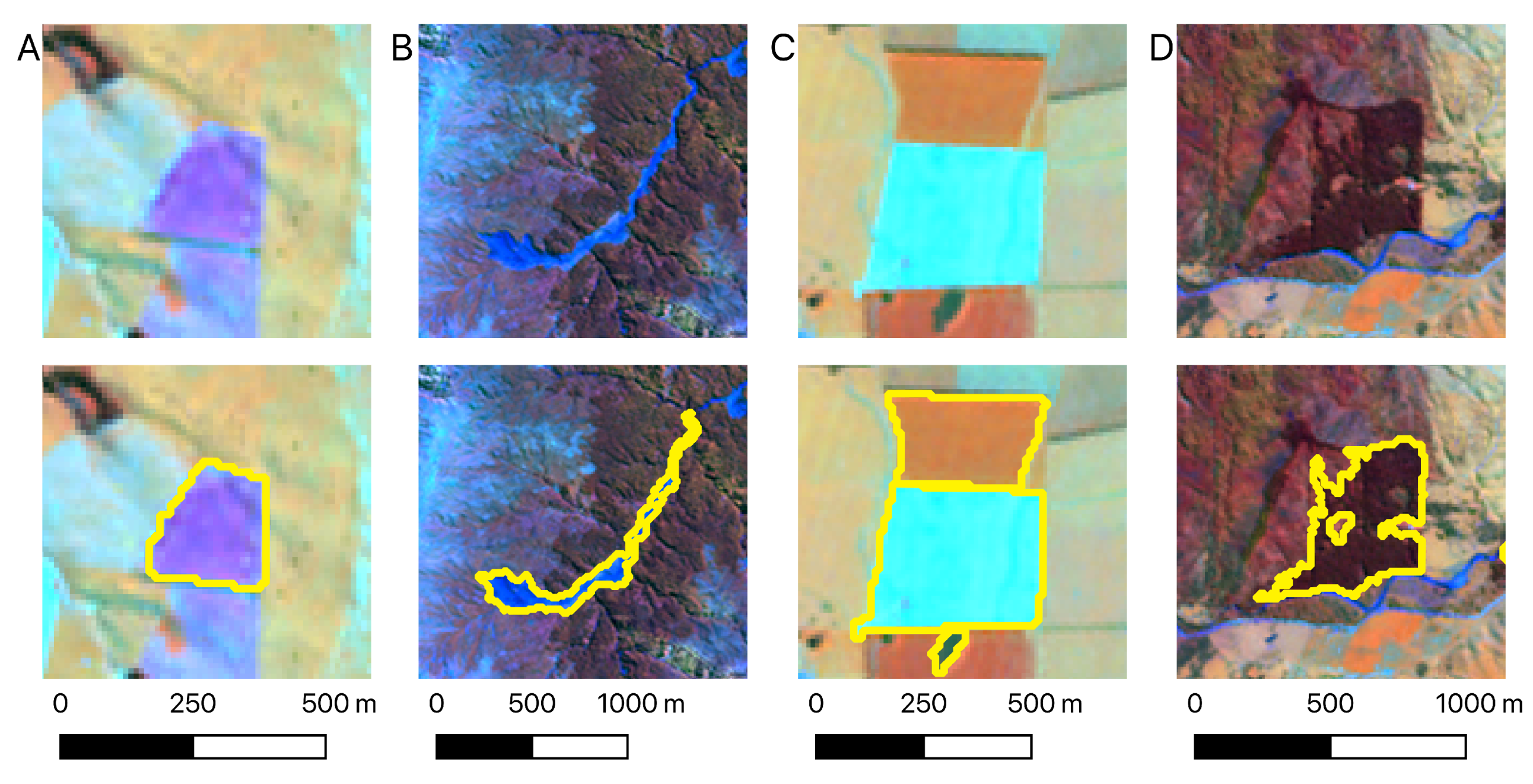
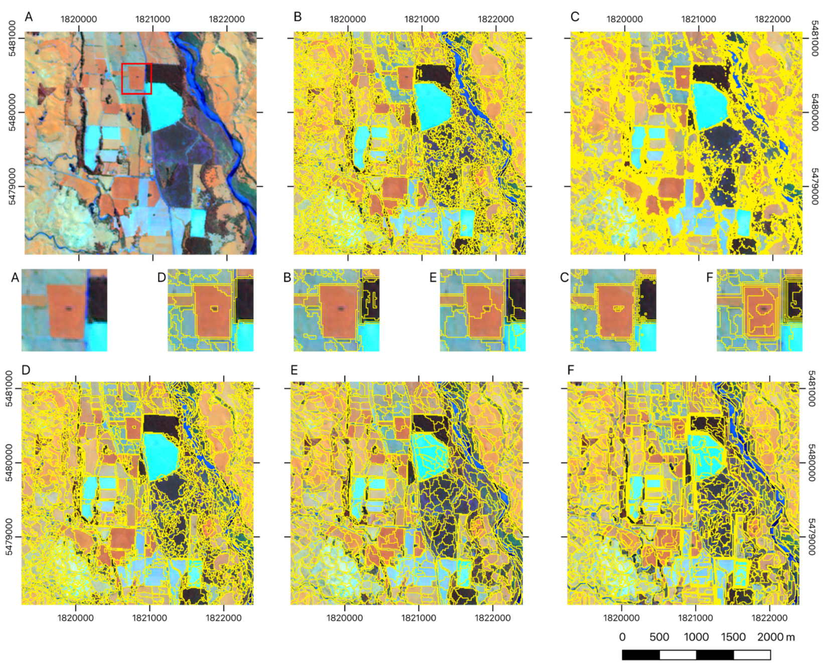
3.1. Visual Assessment
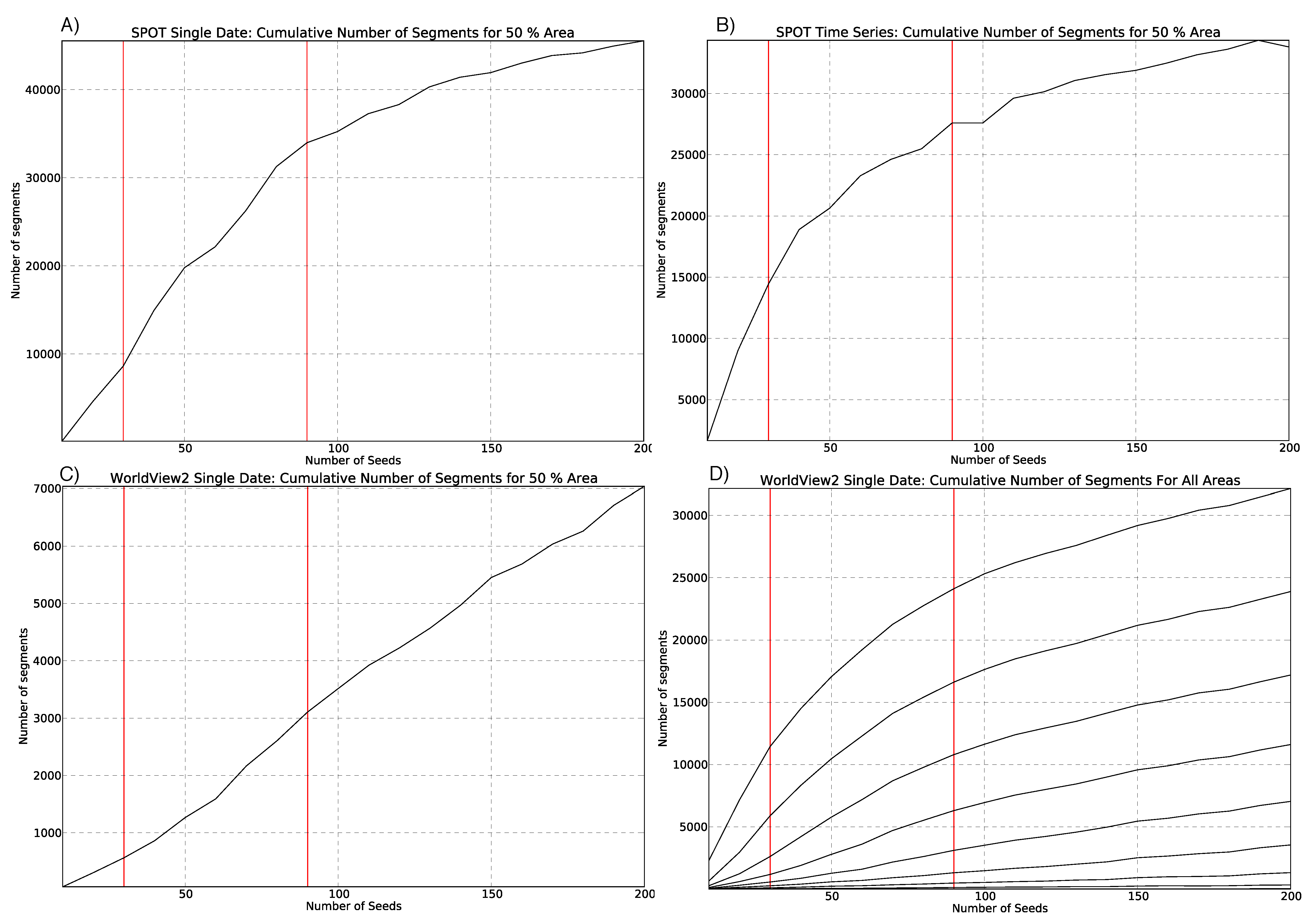
3.2. Parameterisation
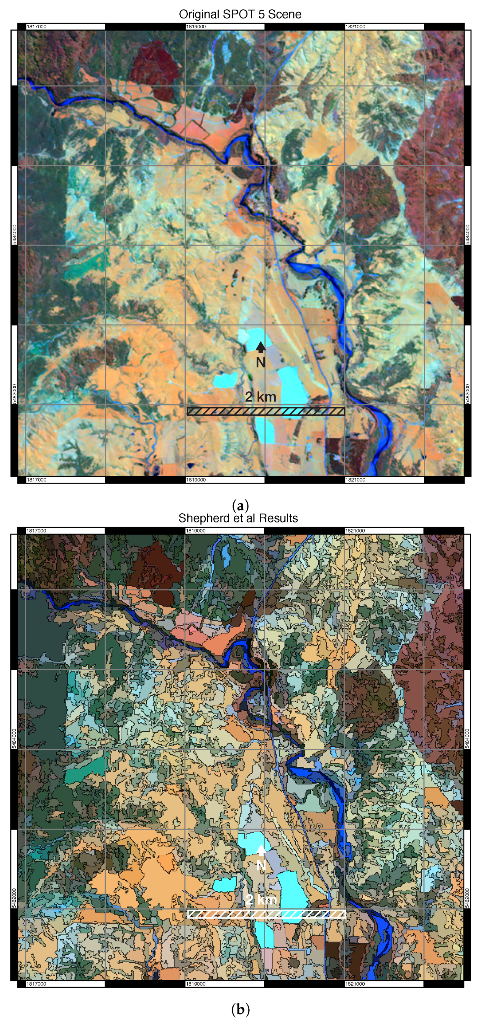
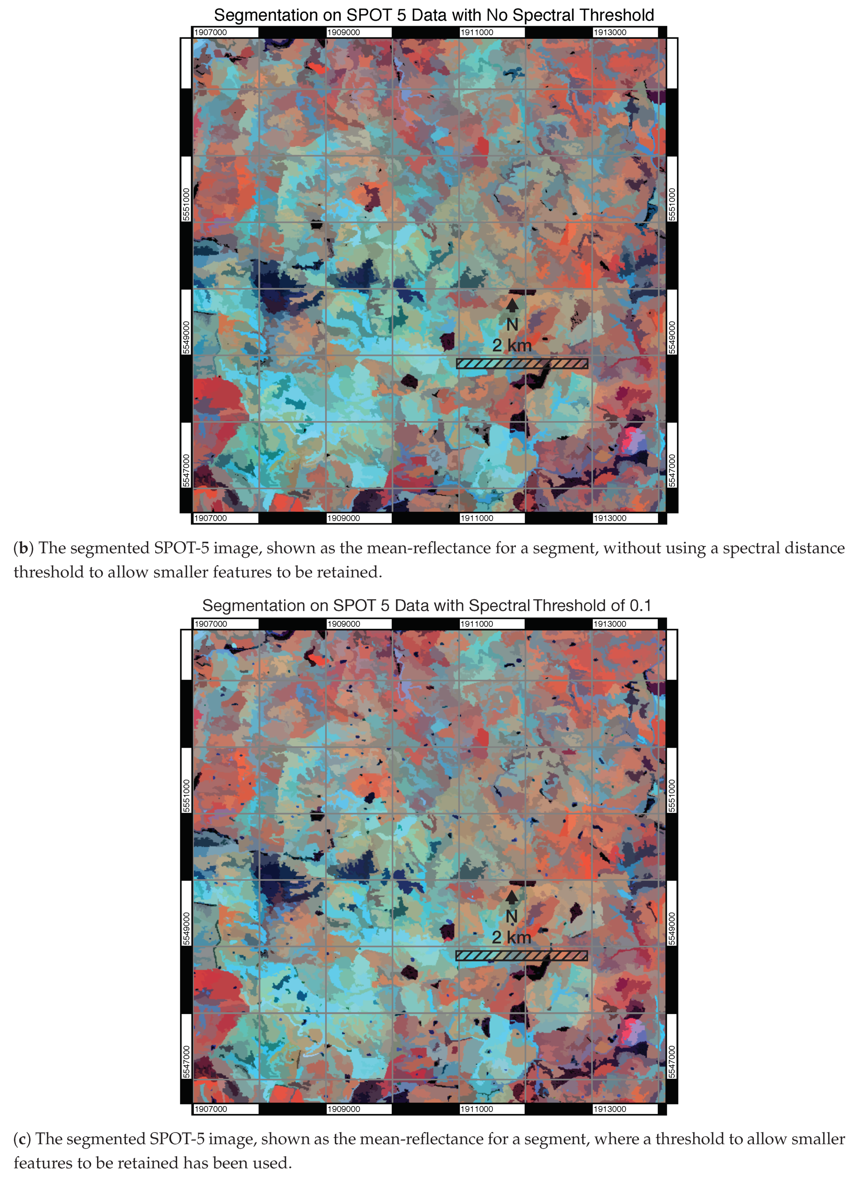
3.3. Comparison to Other Algorithms
4. Discussion
5. Conclusions
Author Contributions
Funding
Conflicts of Interest
References
- Lucas, R.; Rowlands, A.; Brown, A.; Keyworth, S.; Bunting, P. Rule-based classification of multi-temporal satellite imagery for habitat and agricultural land cover mapping. ISPRS J. Photogramm. Remote Sens. 2007, 62, 165–185. [Google Scholar] [CrossRef]
- Lucas, R.; Medcalf, K.; Brown, A.; Bunting, P.; Breyer, J.; Clewley, D.; Keyworth, S.; Blackmore, P. Updating the Phase 1 habitat map of Wales, UK, using satellite sensor data. ISPRS J. Photogramm. Remote Sens. 2011, 66, 81–102. [Google Scholar] [CrossRef]
- Blaschke, T. Object based image analysis for remote sensing. ISPRS J. Photogramm. Remote Sens. 2010, 65, 2–16. [Google Scholar] [CrossRef]
- Lobo, A. Image segmentation and discriminant analysis for the identification of land cover units in ecology. IEEE Trans. Geosci. Remote Sens. 1997, 35, 1136–1145. [Google Scholar] [CrossRef]
- Stuckens, J.; Coppin, P.; Bauer, M. Integrating contextual information with per-pixel classification for improved land cover classification. Remote Sens. Environ. 2000, 71, 282–296. [Google Scholar] [CrossRef]
- Fuller, R.; Smith, G.; Sanderson, J.; Hill, R.; Thomson, A. The UK Land Cover Map 2000: Construction of a parcel-based vector map from satellite images. Cartogr. J. 2002, 39, 15–25. [Google Scholar] [CrossRef]
- Tarabalka, Y.; Benediktsson, J.; Chanussot, J. Spectral-Spatial Classification of Hyperspectral Imagery Based on Partitional Clustering Techniques. IEEE Trans. Geosci. Remote Sens. 2009, 47, 2973–2987. [Google Scholar] [CrossRef]
- Definiens. eCognition Version 5 Object Oriented Image Analysus User Guide; Technical Report; Definiens AG: Munich, Germany, 2005. [Google Scholar]
- Carleer, A.P.; Debeir, O.; Wolff, E. Assessment of Very High Spatial Resolution Satellite Image Segmentations. Photogramm. Eng. Remote Sens. 2005, 71. [Google Scholar] [CrossRef]
- Fu, K.S.; Mui, J.K. A survey on image segmentation. Pattern Recognit. 1981, 13, 3–16. [Google Scholar] [CrossRef]
- Haralick, R.M.; Shapiro, L.G. Image segmentation techniques. Comput. Vis. Graph. Image Process. 1985, 29, 100–132. [Google Scholar] [CrossRef]
- Pal, N.; Pal, S. A review on image segmentation techniques. Pattern Recognit. 1993, 26, 1277–1294. [Google Scholar] [CrossRef]
- Cheng, H.; Jiang, X.; Sun, Y.; Wang, J. Color image segmentation: Advances and prospects. Pattern Recognit. 2001, 34, 2259–2281. [Google Scholar] [CrossRef]
- Dey, V.; Zhang, Y.; Zhong, M. A review on image segmentation techniques with remote sensing perspective. In Proceedings of the ISPRS TC VII Symposium—100 Years ISPRS, Vienna, Austria, 5–7 July 2010; Volume 38, pp. 5–7. [Google Scholar]
- Chen, Q.; Luo, J.; Zhou, C.; Pei, T. A hybrid multi-scale segmentation approach for remotely sensed imagery. In Proceedings of the 2003 IEEE International Geoscience and Remote Sensing Symposium, Toulouse, France, 21–25 July 2003; Volume 6, pp. 3416–3419. [Google Scholar]
- Tilton, J.C. Image segmentation by region growing and spectral clustering with a natural convergence criterion. In Proceedings of the IEEE International Geoscience and Remote Sensing Symposium Proceedings (IGARSS), Seattle, WA, USA, 6–10 July 1998; Volume 4, pp. 1766–1768. [Google Scholar]
- Soille, P. Constrained connectivity for hierarchical image partitioning and simplification. IEEE Trans. Pattern Anal. Mach. Intell. 2008, 30, 1132–1145. [Google Scholar] [CrossRef] [PubMed]
- Ghamisi, P. A Novel Method for Segmentation of Remote Sensing Images based on Hybrid GAPSO. Int. J. Comput. Appl. 2011, 29, 7–14. [Google Scholar] [CrossRef]
- Wang, Z.; Jensen, J.R.; Im, J. An automatic region-based image segmentation algorithm for remote sensing applications. Environ. Model. Softw. 2010, 25, 1149–1165. [Google Scholar] [CrossRef]
- Yang, Y.; Han, C.; Han, D. A Markov Random Field Model-based Fusion Approach to Segmentation of SAR and Optical Images. In Proceedings of the IEEE International Geoscience and Remote Sensing Symposium (IGARSS), Boston, MA, USA, 7–11 July 2008; Volume 4. [Google Scholar]
- Zhao, F.; Jiao, L.; Liu, H. Spectral clustering with fuzzy similarity measure. Digit. Signal Process. 2011, 21, 701–709. [Google Scholar] [CrossRef]
- Tasdemir, K. Neural network based approximate spectral clustering for remote sensing images. In Proceedings of the IEEE International Geoscience and Remote Sensing Symposium (IGARSS), Vancouver, BC, Canada, 24–29 July 2011; pp. 2884–2887. [Google Scholar]
- Tarabalka, Y.; Chanussot, J.; Benediktsson, J. Segmentation and classification of hyperspectral images using watershed transformation. Pattern Recognit. 2010, 43, 2367–2379. [Google Scholar] [CrossRef]
- El Zaart, A.; Ziou, D.; Wang, S.; Jiang, Q. Segmentation of SAR images. Pattern Recognit. 2002, 35, 713–724. [Google Scholar] [CrossRef]
- Brunner, D.; Soille, P. Iterative area filtering of multichannel images. Image Vis. Comput. 2007, 25, 1352–1364. [Google Scholar] [CrossRef]
- Weber, J.; Petitjean, F.; Gançarski, P. Towards Efficient Satellite Image Time Series Analysis: Combination of Dynamic Time Warping and Quasi-Flat Zones. In Proceedings of the IEEE International Geoscience and Remote Sensing Symposium (IGARSS), Munich, Germany, 22–27 July 2012. [Google Scholar]
- Culvenor, D. TIDA: An algorithm for the delineation of tree crowns in high spatial resolution remotely sensed imagery. Comput. Geosci. 2002, 28, 33–44. [Google Scholar] [CrossRef]
- Baatz, M.; Schäpe, A. Multiresolution segmentation: An optimization approach for high quality multi-scale image segmentation. J. Photogramm. Remote Sens. 2000, 58, 12–23. [Google Scholar]
- Lucchese, L.; Mitra, S.K. Unsupervised segmentation of color images based on k-means clustering in the chromaticity plane. In Proceedings of the IEEE Workshop on Content-Based Access of Image and Video Libraries (CBAIVL’99), Fort Collins, CO, USA, 22 June 1999. [Google Scholar]
- Rouse, J.; Haas, R.; Schell, J.; Deering, D. Monitoring vegetation systems in the Great Plains with ERTS. In Proceedings of the NASA Goddard Space Flight Center, 3d ERTS-1 Symposium (NASA SP-351 I), Greenbelt, MD, USA, 1 January 1974; pp. 309–317. [Google Scholar]
- Zhang, H.; Fritts, J.E.; Goldman, S.A. Image segmentation evaluation: A survey of unsupervised methods. Comput. Vis. Image Underst. 2008, 110, 260–280. [Google Scholar] [CrossRef]
- Costa, H.; Foody, G.M.; Boyd, D. Supervised methods of image segmentation accuracy assessment in land cover mapping. Remote Sens. Environ. 2018, 205, 338–351. [Google Scholar] [CrossRef]
- Novack, T.; Fonseca, L.; Kux, H. Quantitative comparison of segmentation results from ikonos images sharpened by different fusion and interpolation techniques. In Proceedings of the GEOgraphic Object Based Image Analysis for the 21st Century (GEOBIA), Calgary, AB, Canada, 5–8 August 2008. [Google Scholar]
- Neubert, M.; Herold, H. Evaluation of remote sensing image segmentation quality—Further results and concepts. In Proceedings of the Bridging Remote Sensing and GIS 1st International Conference on Object-Based Image Analysis (OBIA), Salzburg, Austria, 4–5 July 2006. [Google Scholar]
- Neubert, M.; Herold, H. Assessment of remote sensing image segmentation quality. In Proceedings of the GEOgraphic Object Based Image Analysis for the 21st Century (GEOBIA), Calgary, AB, Canada, 5–8 August 2008. [Google Scholar]
- Zhang, X.; Feng, X.; Xiao, P.; He, G.; Zhu, L. Segmentation quality evaluation using region-based precision and recall measures for remote sensing images. ISPRS J. Photogramm. Remote Sens. 2015, 102, 73–84. [Google Scholar] [CrossRef]
- Marcal, A.R.S.; Rodrigues, S.A. A framework for the evalulation of multi-spectral image segmentation. In Proceedings of the GEOgraphic Object Based Image Analysis for the 21st Century (GEOBIA), Calgary, AB, Canada, 5–8 August 2008. [Google Scholar]
- Johnson, B.; Xie, Z. Unsupervised image segmentation evaluation and refinement using a multi-scale approach. ISPRS J. Photogramm. Remote Sens. 2011, 66, 473–483. [Google Scholar] [CrossRef]
- Shepherd, J.D.; Dymond, J.R. Correcting satellite imagery for the variance of reflectance and illumination with topography. Int. J. Remote Sens. 2003, 24, 3503–3514. [Google Scholar] [CrossRef]
- MacQueen, J. Some methods for classification and analysis of multivariate observations. In Fifth Berkeley Symposium on Mathematical Statistics and Probability; University of California Press: Berkeley, CA, USA, 1967; Volume 1, pp. 281–297. [Google Scholar]
- Ball, G.; Hall, D. A clustering technique for summarizing multivariate data. Behav. Sci. 1967, 12, 153–155. [Google Scholar] [CrossRef]
- Comaniciu, D.; Meer, P. Mean shift: A robust approach toward feature space analysis. IEEE Trans. Pattern Anal. Mach. Intell. 2002, 24, 603–619. [Google Scholar] [CrossRef]
- Ward, J.H., Jr. Hierarchical Grouping to Optimize an Objective Function. J. Am. Stat. Assoc. 1963, 58, 236–244. [Google Scholar] [CrossRef]
- Bezdek, J.C. Fuzzy Mathematics in Pattern Classification. Ph.D. Thesis, Cornell University, Ithaca, NY, USA, 1963. [Google Scholar]
- Dymond, J.R.; Shepherd, J.D.; Newsome, P.F.; Gapare, N.; Burgess, D.W.; Watt, P. Remote sensing of land-use change for Kyoto Protocol reporting: The New Zealand case. Environ. Sci. Policy 2012, 16, 1–8. [Google Scholar] [CrossRef]
- Lucas, R.; Clewley, D.; Accad, A.; Butler, D.; Armston, J.; Bowen, M.; Bunting, P.; Carreiras, J.; Dwyer, J.; Eyre, T.; et al. Mapping forest growth stage in the Brigalow Belt Bioregion of Australia through integration of ALOS PALSAR and Landsat-derived Foliage Projected Cover (FPC) data. Remote Sens. Environ. 2014, 155, 42–57. [Google Scholar] [CrossRef]
- Michel, J.; Feuvrier, T.; Inglada, J. Reference algorithm implementations in OTB: Textbook cases. IEEE Int. Geosci. Remote Sens. Symp. 2009. [Google Scholar] [CrossRef]
- Chaabouni-Chouayakh, H.; Datcu, M. Coarse-to-fine approach for urban area interpretation using TerraSAR-X data. IEEE Geosci. Remote Sens. Soc. Newsl. 2010, 7, 78–82. [Google Scholar] [CrossRef]
- Chehata, N.; Orny, C.; Boukir, S.; Guyon, D.; Wigneron, J.P. Object-based change detection in wind storm-damaged forest using high-resolution multispectral images. Int. J. Remote Sens. 2014, 35, 4758–4777. [Google Scholar] [CrossRef]
- Bellakanji, A.C.; Zribi, M.; Lili-Chabaane, Z.; Mougenot, B. Forecasting of Cereal Yields in a Semi-arid Area Using the Simple Algorithm for Yield Estimation (SAFY) Agro-Meteorological Model Combined with Optical SPOT/HRV Images. Sensors 2018, 18, 2138. [Google Scholar] [CrossRef]
- Mikes, S.; Haindl, M. Benchmarking of remote sensing segmentation methods. IEEE J. Sel. Top. Appl. Earth Obs. Remote Sens. 2015, 8, 2240–2248. [Google Scholar] [CrossRef]
- Vedaldi, A.; Soatto, S. Quick shift and kernel methods for mode seeking. In European Conference on Computer Vision; Springer: Berlin/Heidelberg, Germany, 2008. [Google Scholar]
- Felzenszwalb, P.; Huttenlocher, D. Efficient graph-based image segmentation. Int. J. Comput. Vis. 2004, 59, 167–181. [Google Scholar] [CrossRef]
- Bunting, P.; Clewley, D.; Lucas, R.M.; Gillingham, S. The Remote Sensing and GIS Software Library (RSGISLib). Comput. Geosci. 2014, 62, 216–226. [Google Scholar] [CrossRef]
- Scarth, P.; Armston, J.; Lucas, R.; Bunting, P. A Structural Classification of Australian Vegetation Using ICESat/GLAS, ALOS PALSAR, and Landsat Sensor Data. Remote Sens. 2019, 11, 147. [Google Scholar] [CrossRef]
- Clewley, D.; Bunting, P.; Shepherd, J.; Gillingham, S.; Flood, N.; Dymond, J.; Lucas, R.; Armston, J.; Moghaddam, M. A Python-Based Open Source System for Geographic Object-Based Image Analysis (GEOBIA) Utilizing Raster Attribute Tables. Remote Sens. 2014, 6, 6111–6135. [Google Scholar] [CrossRef]
- Bunting, P.; Gillingham, S. The KEA image file format. Comput. Geosci. 2013, 57, 54–58. [Google Scholar] [CrossRef]


| Sampling (Pixels) | Time (Minutes:Seconds) |
|---|---|
| 100% | 17:14 |
| 50% | 11:10 |
| 20% | 04:03 |
| 1% | 02:39 |
| 0.1% | 00:08 |
| Sensor | Year (s) | Image Size | Pixel Resolution |
|---|---|---|---|
| Worldview2 | July 2011 *, November 2011 | 2 m | |
| SPOT5 | 2008, 2012 * | 10 m | |
| Landsat 4/7 | 1990, 2002 * | 15 m |
| Algorithm | Parameters | Number of Segmentations |
|---|---|---|
| eCognition | scale: [10–100], shape: [0–1], compact.: [0–1] | 1210 |
| Mean-Shift | range radius; [5–25], convergence thres.: [0.01–0.5], max. iter.: [10–500], min. size: [10–500] | 625 |
| Felzenszwalb | scale: [0.25–10], sigma: [0.2–1.4], min. size: [5–500] | 343 |
| Quickshift | ratio: [0.1–1], kernel size: [1–20], max. dist.: [1–30], sigma: [0–5] | 1500 |
| Shepherd et al. | k: [5–120], d: [10–10,000], min. size: [5–200] | 540 |
| Algorithm | Parameters | Rank | f | Precision | Recall | ||||||
|---|---|---|---|---|---|---|---|---|---|---|---|
| Shepherd et al. | k: 60, d: 10,000, min. size: 10 | 1 | 0.74 | 0.85 | 0.84 | 0.86 | 0.97 | 1.01 | 0.90 | 0.99 | 0.98 |
| Quickshift | ratio: 0.75, kernel size: 10, max. dist.: 5, sigma: 0, lab colour space. | 86 | 0.64 | 0.73 | 0.80 | 0.68 | 0.94 | 0.92 | 0.86 | 0.99 | 0.98 |
| Mean-Shift | range radius; 15, convergence thres.: 0.2, max. iter.: 100, min. size: 10 | 253 | 0.56 | 0.61 | 0.55 | 0.70 | 0.93 | 0.95 | 0.87 | 0.96 | 0.94 |
| eCognition | scale: 10, shape: 0.7, compact.: 0.2 | 411 | 0.49 | 0.52 | 0.57 | 0.48 | 0.95 | 0.99 | 0.92 | 0.95 | 0.93 |
| Felzenszwalb | scale: 10, sigma: 12, min. size: 20 | 539 | 0.47 | 0.46 | 0.49 | 0.43 | 1.10 | 1.14 | 1.04 | 1.17 | 1.04 |
© 2019 by the authors. Licensee MDPI, Basel, Switzerland. This article is an open access article distributed under the terms and conditions of the Creative Commons Attribution (CC BY) license (http://creativecommons.org/licenses/by/4.0/).
Share and Cite
Shepherd, J.D.; Bunting, P.; Dymond, J.R. Operational Large-Scale Segmentation of Imagery Based on Iterative Elimination. Remote Sens. 2019, 11, 658. https://doi.org/10.3390/rs11060658
Shepherd JD, Bunting P, Dymond JR. Operational Large-Scale Segmentation of Imagery Based on Iterative Elimination. Remote Sensing. 2019; 11(6):658. https://doi.org/10.3390/rs11060658
Chicago/Turabian StyleShepherd, James D., Pete Bunting, and John R. Dymond. 2019. "Operational Large-Scale Segmentation of Imagery Based on Iterative Elimination" Remote Sensing 11, no. 6: 658. https://doi.org/10.3390/rs11060658
APA StyleShepherd, J. D., Bunting, P., & Dymond, J. R. (2019). Operational Large-Scale Segmentation of Imagery Based on Iterative Elimination. Remote Sensing, 11(6), 658. https://doi.org/10.3390/rs11060658