Article

Support Vector Machine Accuracy Assessment for Extracting Green Urban Areas in Towns

1
Faculty of Geotechnical Engineering, University of Zagreb, Hallerova aleja 7, 42000 Varaždin, Croatia
2
Faculty of Geodesy, University of Zagreb, Kačićeva 26, 10000 Zagreb, Croatia
*
Author to whom correspondence should be addressed.
Remote Sens. 2019, 11(6), 655; https://doi.org/10.3390/rs11060655
Submission received: 22 January 2019 / Revised: 2 March 2019 / Accepted: 15 March 2019 / Published: 18 March 2019
(This article belongs to the Section Urban Remote Sensing)

Abstract

:
The most commonly used model for analyzing satellite imagery is the Support Vector Machine (SVM). Since there are a large number of possible variables for use in SVM, this paper will provide a combination of parameters that fit best for extracting green urban areas from Copernicus mission satellite images. This paper aims to provide a combination of parameters to extract green urban areas with the highest degree of accuracy, in order to speed up urban planning and ultimately improve town environments. Two different towns in Croatia were investigated, and the results provide an optimal combination of parameters for green urban areas extraction with an overall kappa index of 0.87 and 0.89, which demonstrates a very high classification accuracy.

Graphical Abstract

1. Introduction

The green urban areas infrastructure approach considers maximizing physical and functional connectivity while optimizing multi-functionality in terms of social, ecological, and economic benefits [1], as well as resilience through landscape diversity [2,3].
Green urban areas are important for urban planning and improving the urban environment [4]. For this, quick access to data is important to enable up-to-date planning and decision-making. Green infrastructure that incorporates urban nature is important for physical and mental health benefits [5]. Several authors have provided papers on green infrastructure and spatial planning [5,6,7], and they all agree that green urban infrastructure has an important role in the quality of a city’s lifestyle. Satellite imagery is the fastest method for data collection for urban planning. Since the first development of satellite imagery, many studies have investigated extracting various types of vegetation information. The authors in [8] combined IKONOS and Landsat ETM+ data in order to map structural parameters and the species composition of riparian vegetation. The authors in [9] used GeoEye-1 high spatial resolution satellite data to map canopy mortality caused by a pine beetle outbreak. They concluded that high-resolution imagery is a useful tool to map such natural disasters. Similar work to [8] was conducted by the authors in [10] in order to distinguish forest species in South Africa, but their work was based on Worldview-2 multispectral bands. The authors in [11] used WorldView-2, RapidEye, and PlanetScope data to detect urban vegetation based on land cover classification. The authors in [12] used Sentinel-2 data to visualize bark-beetle-damaged forests in Croatia, and the authors in [13] tested object-based and pixel-based methods on Sentinel-2 imagery for two forest sites in Germany. The authors in [12,13] stated that Sentinel-2 data indicate a high potential for applied forestry and vegetation analysis. The authors in [14] used unsupervised machine learning to map landscape soils and vegetation components from satellite imagery. The authors in [15] used machine learning classification in order to map vegetation and land use types. As seen from the abovementioned literature, a lot of work has been done with machine learning to extract vegetation information.
Machine learning is a very deep and complicated field. However, many different types of machine learning methods are intended to provide the same outcome, starting with known examples to develop a pattern and applying the pattern to a dataset with no familiar data [16]. The basics of most machine learning methods are as follows:
  • Start with known datasets;
  • Train the machine learning algorithm on known datasets (training sets);
  • Obtain the dataset for which one wants to know an answer (test sets); and
  • Pass the test set through the trained algorithm to provide the result [16].
Recently, machine learning models have been proposed for various classification and regression tasks using satellite imagery [17]. Different to typical statistical approaches, machine learning techniques are usually free from data assumptions and have proven to be useful in nonlinear behavior modeling [17].
Support vector machines were proposed in [18], following which they were studied thoroughly due to their high-quality results in image recognition. According to [19,20], the most common satellite image classification machine learning modules are ISODATA, the K-Means algorithm, and Support Vector Machine (SVM). Several books have been published on SVM [21,22,23]. Support Vector Machine is an abstract machine learning algorithm that learns from a training dataset and attempts to generalize and make a correct prediction on new datasets [21]. The library for support vector machines (LIBSWM) helps users to implement SVM into their applications. LIBSVM supports different SVM formulations for classification, regression, and distribution estimation [24]. Kernels are commonly used in conjunction with support vector machine modules. The most commonly used kernels for image processing are polynomial, radial basis function, and sigmoid kernels [25].
These three kernels are used in combination with SVM modules in this paper. According to [25], the radial basis function kernel should provide the best overall results for green urban areas extraction.
Since the usefulness of combining satellite imagery and machine learning for different types of vegetation has been proven in the abovementioned studies, this paper will offer a particular combination of parameters to extract green urban areas with the highest degree of accuracy.

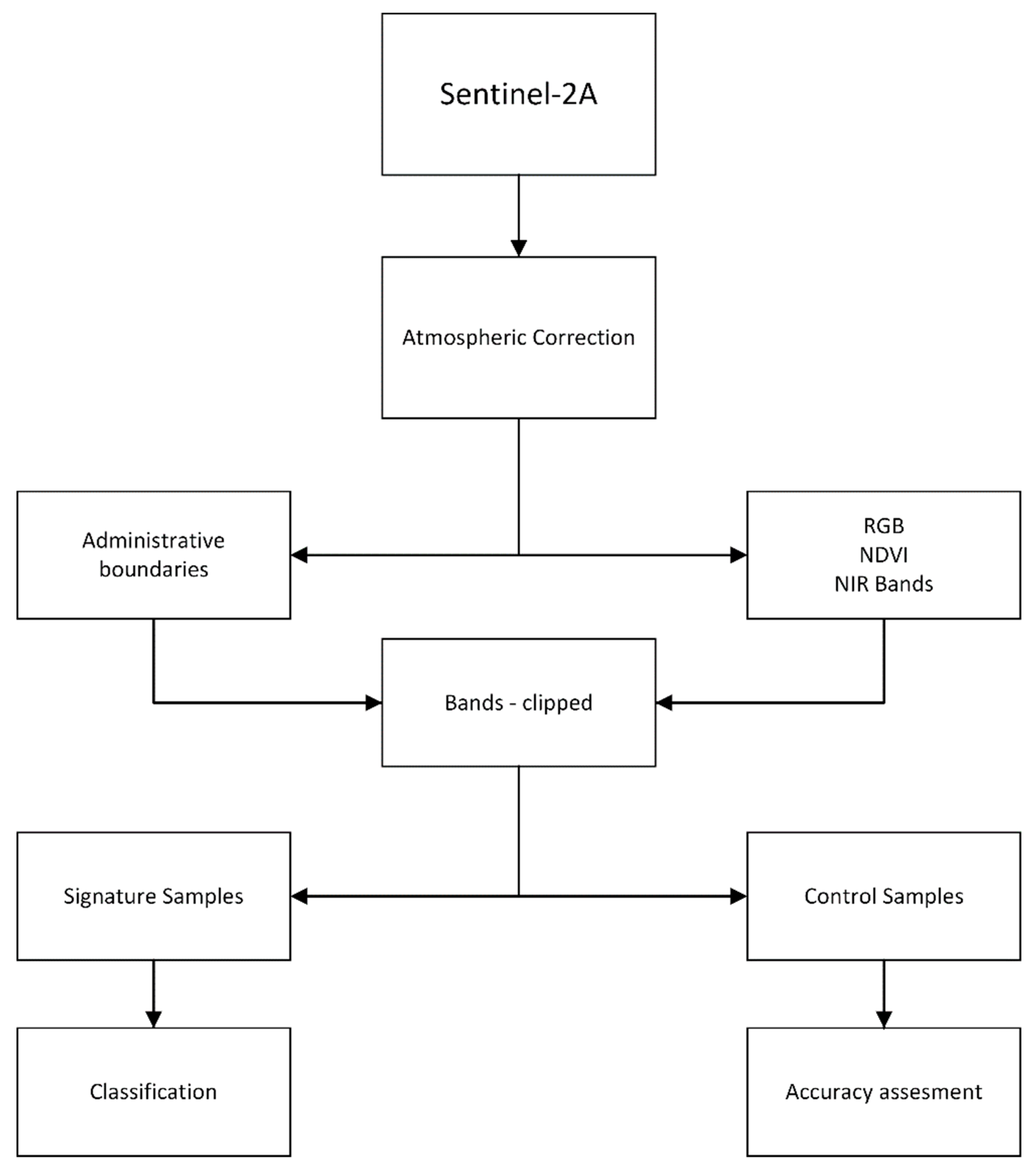
2. Materials and Methods

The study area is located in two towns in Croatia: Varaždin and Osijek. Based on the OpenStreetMap classification, a town is an urban settlement with local importance and a population between 10,000 and 100,000. Both towns have a similar land cover use. Both are located on the River Drava, and the central area is populated with an urban fabric while smaller areas are filled with green urban areas. The wider city centre is populated with arable land, forests, and inland waters. The dominant types of vegetation in Varaždin are forests populated with beech, oak, and chestnut and larger parks with grass and shrubbery. The dominant types of vegetation in Osijek are also parks, but in Osijek there are many swamp plants and linden and oak trees dominate forests. The coordinates for the centre of the study areas of Varaždin and Osijek are shown in Table 1. Study areas with a signature and control samples are presented in Figure 1. The workflow is presented in Figure 2. The first step was to download satellite images from the Copernicus Open Access Hub web page [26].
Downloading images with zero or almost zero cloud coverage was important. The imagery for the Varaždin study area was recorded on 14 August 2016, and the imagery for the Osijek study area was recorded on 29 August 2016. The Sentinel-2A multispectral imager covers 13 spectral bands, from 443 to 2190 nm, with a swath width of 290 km and a spatial resolution of 10 m (four visible and near-infrared bands), 20 m (six red edge and shortwave infrared bands), and 60 m (three atmospheric correction bands). After the images were downloaded, atmospheric correction was performed. The atmospheric correction was performed using the Dark Object Subtraction 1 (DOS1) correction. DOS is a family of image-based corrections. Image-based corrections have a lower accuracy than physical-based corrections. For this research, the DOS1 correction was useful as it improves the estimation of land surface reflectance on satellite images [27]. Administrative areas were downloaded from [28], and images were clipped on the Varaždin and Osijek administrative areas. The next step was to conduct classification processes. The study areas were separated into five classes according to Corine Land Cover [29]: inland water, forests, green urban areas, arable land, and urban fabric. Signature and control samples were selected based on RGB color composition, normalized difference vegetation index (NDVI), combining the infrared band with the green and blue bands, and also experience of living in these two towns. For the Varaždin study area, there were 69 signature samples and 26 control samples. For the Osijek study area, there were 41 signature samples and 26 control samples.
The classification was made by combining two support vector machine modules and using three kernel types. The kernels used in this study were [30]:
• The polynomial kernel:
K ( u , v ) = ( γ × u , v + c o e f 0 ) d
• The radial basis function (RBF) kernel:
K ( u , v ) = exp γ × | u v | 2
• The sigmoid kernel:
K ( u , v ) = tanh ( γ × u , v + c o e f 0 )
where coef 0 is a coefficient, γ is the gamma, and d is the degree.
The parameters and combinations used in the classification are contained in Table 2. Where the values are left out, the default value was used. In Table 2, abbreviations for kernels are used. “Pol” is the polynomial kernel, “RBF” is the radial basis function kernel, and “Sig” is the sigmoid kernel. The factor C parameter allows one to trade off training error versus model complexity. A small value for C will increase the number of training errors, while a large C value will lead to behavior similar to that of the hard-margin SVM [31]. γ is the free parameter of the radial basis function. If γ is large, then the variance is small, implying that the support vector does not have a widespread influence. Basically, a large γ leads to high-bias and low-variance models, and vice-versa.
According to [32], the error or confusion matrix is the most commonly used accuracy assessment. It shows class types determined from the classified map in rows and class types determined from the reference source in columns. Correctly classified polygons are represented in diagonals, while misclassified polygons are represented in the off-diagonal error matrix [11]. An example of an error matrix is taken from the results of the classification (parameter 7 in Table 2), as shown in Table 3.
Omission and commission errors within the confusion matrix are also considered [11]. A commission error occurs when polygons from other classes are allocated to the reference data [11]. An omission error appears when the polygons of the reference data are allocated to other classes [11]. According to [33], kappa analysis is a powerful method for comparing the differences between diverse error matrices. The accuracy rank for each kappa coefficient is shown in Table 4. The kappa statistic is a measure of the similarity between signature samples and control samples [34]. It indicates that a moderate classification accuracy has a similarity between 41 and 60%. In the same manner, high and very high classification accuracy are presented in Table 4. In Table 5, the commission error is labeled as C and the omission error is labeled as O.

3. Results

After obtaining the signature and control samples (Figure 1), the classification was performed. The parameters for the classification are shown in Table 2. Out of 14 tested combinations, only a few produced satisfying results. Classification using the polynomial kernel produced results only for the parameters in Column 1 of Table 2. The parameters in Columns 2, 3, and 4 of Table 2 did not produce any outputs because the maximum number of iterations was exceeded. Classification using the parameters in Columns 5 and 6 produced similar results to those from classification using the parameters in Columns 7 and 8. Classification using the sigmoid kernel was low of quality, with a kappa range of 0.19–0.41. Classification using the ν-SVR produced similar results to those from classification using the C-SVR. The results of classification using the parameters in Columns 1, 7, 8, 9, and 13 from Table 2 are presented in Table 5, Table 6, and Figure 3, Figure 4, Figure 5 and Figure 6. As shown in Table 5, the estimated kappa for class number 3, which represents vegetation, is marked in green. The best estimated kappa for vegetation extraction was determined using the polynomial kernel. However, the overall classification accuracy was rather low compared to that of other parameters.
Figure 3 and Figure 4 show the results of classification using different parameters. As mentioned above, only a few of the classification parameters produced the desired results, and only five sets of results are shown in Figure 3. In Figure 3, it can be seen that the vegetation has been correctly classified and that, in some areas, the classification process had issues separating water from vegetation as well as soil from buildings. This is an expected issue, since these classes have a similar spectral signature.
Figure 5 and Figure 6 show the estimated kappa for every parameter in graphical form. Since the kappa is an indicator of the quality of classification, it is obvious that the classification using the radial basis function kernel produces the best results. However, there is a small difference between C-SVM and ν-SVM.
Figure 7 and Figure 8 show how the choice of parameters affects the classification and pixel distribution for each class. If one compares parameters 7 and 8, it is obvious that the only difference is in the classification of Class 3 (green urban areas) and Class 5 (urban fabric). The results determined that the highest kappa is in parameter 1 and the highest estimated kappa for Class 3 is in parameter 1. However, parameter 1 has only four classes and, therefore, could not be evaluated. From this, we determined that the best overall combination of parameters is the parameters in Column 7 in Table 2 for both study areas.

4. Discussion

According to [25], the best kernel for classification in general is the radial basis function kernel because it produces the highest overall accuracy and highest overall kappa. We have confirmed this finding, adding that the radial basis function is also the best kernel for green urban areas extraction. The authors in [35] found that the best overall accuracy is attained using the radial basis function where γ equals 1 and C equals 28, with an overall accuracy of 92.67. However, the authors in [25] used synthetic aperture radar (SAR) data for their study, and the authors in [35] used hyperspectral data for their study. Since the spectral characteristics of SAR and hyperspectral data are both different from Sentinel-2A data, these two studies cannot be directly compared to our study, but can show tendencies and guidelines for similar research. The authors in [36] found that SVM produces the highest accuracy during classification on Sentinel 2 imagery. The authors in [37] showed that the polynomial kernel produced the best overall accuracy for the classification of RapidEye multispectral imagery. In accordance with [36], we used a support vector machine learning module to classify Sentinel 2 imagery. However, in contrast to [37], we found that the highest accuracy was obtained with the radial basis function kernel for Sentinel 2 imagery classification. We also found that Sentinel 2 imagery is useful for green urban areas extraction and, with the right combination of parameters, can provide a classification with a high level of accuracy. The usefulness of Sentinel 2 imagery has already been confirmed in different analyses for different purposes [12,13,38], and it could also be used for decision-making in urban planning. Further research is proposed using high-resolution imagery produced by an unmanned aerial vehicle combined with Sentinel 2 data in order to improve the model for green urban areas extraction. The improved model should provide a better overall kappa for green urban areas extraction.

5. Conclusions

Urban planning for and increasing the amount of green urban infrastructure are crucial for healthier living. To achieve this effectively, experts have combined machine learning modules with satellite imagery. The development of the Copernicus satellite missions represents a huge advance in land observation due to the increment in spatial resolution. Many analyses have been conducted to determine which of the parameters is most suitable for green urban areas extraction in satellite images. SVM is one of the most commonly used machine learning modules in image classification, and, according to different authors, the most common kernel is the radial basis function. The radial basis function is one of the kernels that produces classifications of the highest quality. In this paper, various combinations of parameters were examined. The results show that, for green urban areas extraction, the highest estimated kappa was obtained using the polynomial kernel and C-SVM; however, the polynomial kernel has a rather poor overall accuracy and should not be used for such classification. The overall highest quality is produced using the radial basis function in combination with C-SVM. However, a satisfying quality is also produced using the ν-SVM in combination with the radial basis function kernel. Further research is proposed to develop a novel model to extract vegetation that combines high-resolution aerial imagery and satellite imagery.

Author Contributions

Conceptualization, D.M. and R.Ž.; methodology, N.K.; software, N.K.; validation, D.M., R.Ž., and M.R.; formal analysis, N.K.; investigation, N.K.; resources, N.K.; data curation, N.K.; writing—original draft preparation, N.K.; writing—review and editing, M.R.; visualization, N.K.; supervision, D.M.

Funding

This research was funded by the Croatian Science Foundation under the project “Geospatial Monitoring of Green Infrastructure by Means of Terrestrial, Airborne and Satellite Imagery”, grant number: IP-2016-06-5621.

Conflicts of Interest

The authors declare no conflict of interest.

References

  1. Mell, I.C. Can you tell a green field from a cold steel rail. Examining the “green” of green infrastructure development. Local Environ. Int. J. Justice Sustain. 2015. [Google Scholar] [CrossRef]
  2. Bird, W. Natural greenspace. Br. J. Gen. Pract. 2007, 57, 69. [Google Scholar] [PubMed]
  3. Dennis, M.; Barlow, D.; Cavan, G.; Id, P.A.C.; Gilchrist, A.; Handley, J.; Id, P.J.; Thompson, J.; Id, K.T.; Wheater, C.P.; et al. Mapping urban green infrastructure: A novel landscape-based approach to incorporating land use and land cover in the mapping of human-dominated systems. Land 2018, 7, 17. [Google Scholar] [CrossRef]
  4. Yang, C.; Huang, H.; Zhang, Y. Comparison of extracting the urban green land from satellite images with multi-resolutions. In Proceedings of the Urban Remote Sensing Event, Shanghai, China, 20–22 May 2009. [Google Scholar] [CrossRef]
  5. Parker, J.; Simpson, G.D. Public green infrastructure contributes to city livability: A systematic quantitative review. Land 2018, 7, 116. [Google Scholar] [CrossRef]
  6. Juane, E. Reflecting on green infrastructure and spatial planning in africa: The complexities, perptions, and y foard. Sustainability 2019, 11, 455. [Google Scholar] [CrossRef]
  7. Green, F.; Policies, I. Predicting land use changes in philadelphia following green infrastructure policies. Land 2019, 8, 28. [Google Scholar] [CrossRef]
  8. Johansen, K.; Phinn, S. Mapping structural parameters and species composition of riparian vegetation using IKONOS and landsat ETM + data in Australian tropical savannahs. Photogramm. Eng. Remote Sens. 2006, 72, 71–80. [Google Scholar] [CrossRef]
  9. Dennison, P.E.; Brunelle, A.R.; Carter, V.A. Assessing canopy mortality during a mountain pine beetle outbreak using GeoEye-1 high spatial resolution satellite data. Remote Sens. Environ. 2010, 114, 2431–2435. [Google Scholar] [CrossRef]
  10. Peerbhay, K.Y.; Mutanga, O.; Ismail, R. Investigating the capability of few strategically placed worldview-2 multispectral bands to discriminate forest species in KwaZulu-Natal, South Africa. IEEE J. Sel. Top. Appl. Earth Obs. Remote Sens. 2014, 7, 307–316. [Google Scholar] [CrossRef]
  11. Gašparović, M.; Dobrinić, D.; Medak, D. Urban vegetation detection based on the land-cover classification of Planetscope, Rapideye and Wordview-2 satellite imagery. In Proceedings of the 18th International Multidisciplinary Scientific Geoconference SGEM, 30 June–9 July 2018. [Google Scholar]
  12. Kranjčić, N.; Župan, R.; Rezo, M. Satellite-based hyperspectral imaging and cartographic visualization of bark beetle forest damage for the city of Čabar. Tech. J. 2018, 12, 39–43. [Google Scholar] [CrossRef]
  13. Wessel, M.; Brandmeier, M.; Tiede, D. Evaluation of Different Machine Learning Algorithms for Scalable Classification of Tree Types and Tree Species Based on Sentinel-2 Data. Remote Sens. 2018, 10, 1419. [Google Scholar] [CrossRef]
  14. Friedel, M.J.; Buscema, M.; Vicente, L.E.; Iwashita, F.; Koga-vicente, A. Mapping fractional landscape soils and vegetation components from hyperion satellite imagery using an unsupervised machine-learning workflow. Int. J. Digit. Earth 2017, 11, 670–690. [Google Scholar] [CrossRef]
  15. Tsai, Y.H.; Stow, D.; Chen, H.L.; Lewison, R.; An, L.; Shi, L. Mapping vegetation and land use types in fanjingshan national nature reserve using google earth engine. Remote Sens. 2018, 10. [Google Scholar] [CrossRef]
  16. Hartshorn, S. Machine Learning With Random Forests And Decision Trees A Visual Guide For Beginners; Amazon Digital Services LCC,410 Terry Avenue North: Seattle, WA, USA, 2016. [Google Scholar]
  17. Sim, S.; Im, J.; Park, S.; Park, H.; Hwan Ahn, M.; Chan, P. Icing detection over east asia from Geostationary satellite data using machine learning approaches. Remote Sens. 2018. [Google Scholar] [CrossRef]
  18. Vapnik, V.N. The Nature of Statistical Learning Theory; Springer: Berlin, Germany, 1995; ISBN 0387987800. [Google Scholar]
  19. Gašparović, M.; Zrinjski, M.; Gudelj, M. Analiza urbanizacije grada Splita. Geod. List 2017, 71. [Google Scholar]
  20. Irvin, B.J.; Ventura, S.J.; Slater, B.K. Fuzzy and isodata classification of landform elements from digital terrain data in Pleasant Valley, Wisconsin. Geoderma 1997, 77, 137–154. [Google Scholar] [CrossRef]
  21. Campbell, C.; Ying, Y. Learning with Support Vector Machines. In Synthesis Lectures on Artificial Intelligence and Machine Learning; Morgan & Claypool Publishers: San Rafael, CA, USA, 2011; ISBN 9781608456161. [Google Scholar]
  22. Schölkopf, B.; Smola, A.J.; Williamson, R.C.; Bartlett, P.L. New support vector algorithms. Neural Comput. 2000, 12, 1207–1245. [Google Scholar] [CrossRef] [PubMed]
  23. Steinwart, I.; Christmann, A. Support Vector Machines; Schölkopf, B., Jordan, M., Kleinberg, J., Eds.; Springer-Verlag: New York, NY, USA, 2008; ISBN 978-0-387-77241-7. [Google Scholar]
  24. Chang, C.-C.; Lin, C.-J. LIBSVM: A library for support vector machines. ACM Trans. Intell. Syst. Technol. 2013, 2. [Google Scholar] [CrossRef]
  25. Yekkehkhany, B.; Safari, A.; Homayouni, S.; Hasanlou, M.A.; Homayouni, S.; Hasanlou, M. A comparison study of different kernel functions for SVM-based classification of multi-temporal polarimetry SAR data. In International Archives of the Photogrammetry, Remote Sensing and Spatial Information Sciences—ISPRS Archives; ISPRS: Hanover, Germany, 2014. [Google Scholar]
  26. Copernicus Open Access Hub. Available online: https://scihub.copernicus.eu/dhus/#/home (accessed on 12 September 2018).
  27. Congedo, L. Semi-Automatic Classification Plugin Documentation. Release 2017, 4, 29. [Google Scholar]
  28. Diva-gis web page. Available online: http://www.diva-gis.org/ (accessed on 12 September 2018).
  29. Agency, E.E. CORINE Land Cover—Technical guide; European Environment Agency: Kobenhavn, Denmark, 2000. [Google Scholar]
  30. Saga-Gis Web Page. Available online: http://www.saga-gis.org/saga_tool_doc/2.2.0/imagery_svm_0.html (accessed on 12 October 2018).
  31. Joachims, T. Learning to Classify Text Using Support Vector Machines; In Science+Business Media, LCC; Springer: Berlin, Germany, 2001; ISBN 978-1-4613-5298-3. [Google Scholar]
  32. Foody, G.M. Status of land cover classification accuracy assessment. Remote Sens. Environ. 2002, 80, 185–201. [Google Scholar] [CrossRef]
  33. Viera, A.J.; Garrett, J.M. Understanding interobserver agreement: The kappa statistic. Fam. Med. 2005, 37. [Google Scholar]
  34. Cracknell, M.J.; Reading, A.M. Geological mapping using remote sensing data: A comparison of fi ve machine learning algorithms, their response to variations in the spatial distribution of training data and the use of explicit spatial information. Comput. Geosci. 2014, 63, 22–33. [Google Scholar] [CrossRef]
  35. Demir, B.; Ertürk, S. Hyperspectral image classification using relevance vector machines. IEEE Geosci. Remote Sens. Lett. 2007, 4, 586–590. [Google Scholar] [CrossRef]
  36. Noi, P.T.; Kappas, M. Comparison of random forest, k-nearest neighbor, and support vector machine classifiers for land cover classification using sentinel-2 imagery. Sensors 2017, 18, 18. [Google Scholar] [CrossRef]
  37. Ustuner, M.; Sanli, F.B.; Dixon, B. Application of support vector machines for landuse classification using high-resolution rapideye images: A sensitivity analysis application of support vector machines for landuse Classification using high-resolution rapideye Images. Eur. J. Remote Sens. 2017, 48, 403–422. [Google Scholar] [CrossRef]
  38. Radoux, J.; Chomé, G.; Jacques, D.C.; Waldner, F.; Bellemans, N.; Matton, N.; Lamarche, C.; D’Andrimont, R.; Defourny, P. Sentinel-2’s potential for sub-pixel landscape feature detection. Remote Sens. 2016, 8, 488. [Google Scholar] [CrossRef]
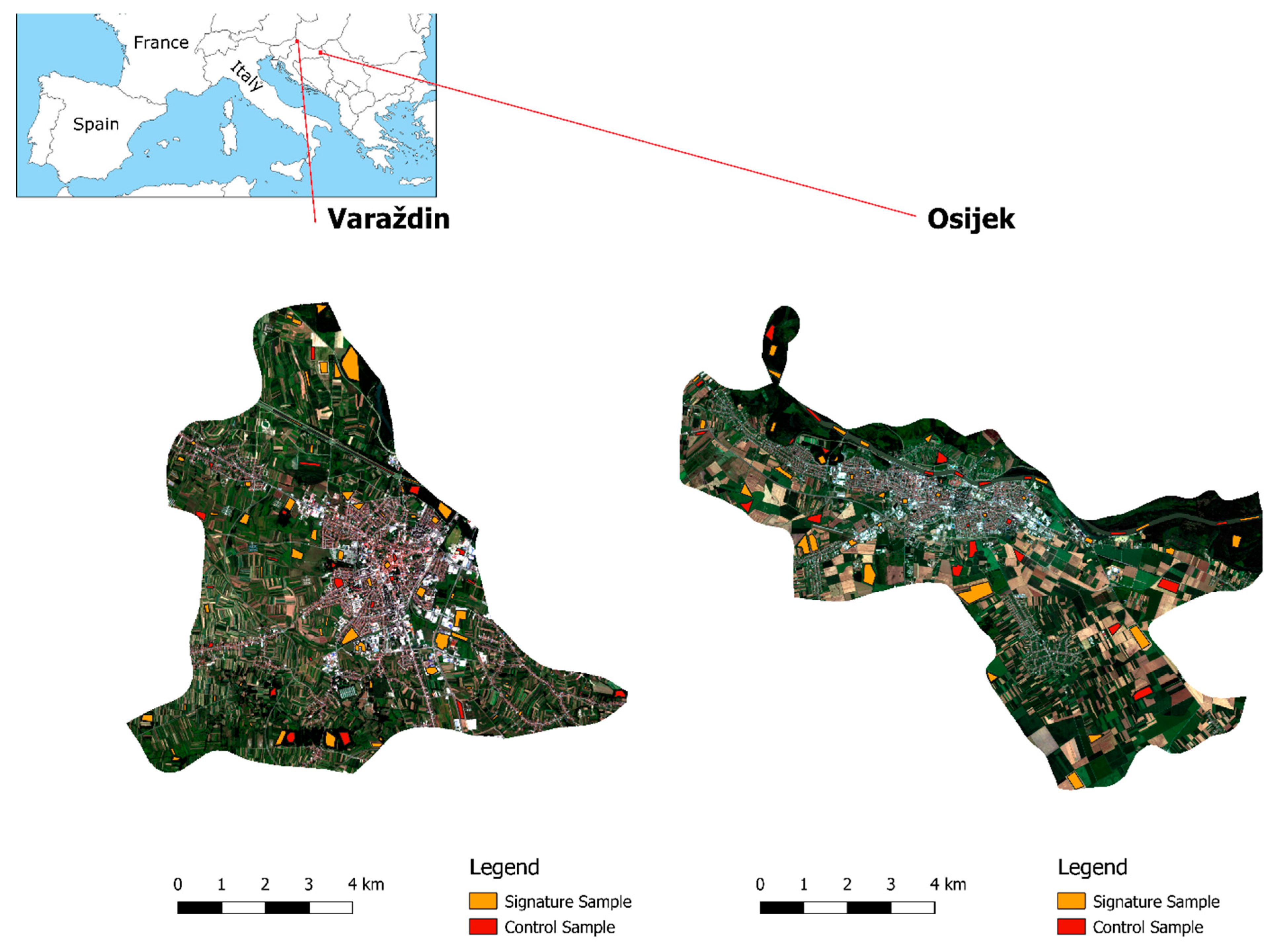
Figure 1. The study area: Varaždin (left); Osijek (right).
Remotesensing 11 00655 g001
Figure 2. The workflow process. NDVI, normalized difference vegetation index; NIR, near-infrared.
Remotesensing 11 00655 g002
Figure 3. Classification results for the Varaždin study area.
Remotesensing 11 00655 g003
Figure 4. Classification results for the Osijek study area.
Remotesensing 11 00655 g004
Figure 5. The estimated kappa for the Varaždin study area.
Remotesensing 11 00655 g005
Figure 6. The estimated kappa for the Osijek study area.
Remotesensing 11 00655 g006
Figure 7. The pixel distribution per class for the Varaždin study area.
Remotesensing 11 00655 g007
Figure 8. The pixel distribution per class for the Osijek study area.
Remotesensing 11 00655 g008
Table 1. The study area coordinates (projection: EPSG 3765 | WGS84).
E(m) | φ (d° m′ s″)N(m) | λ (d° m′ s″)
Varaždin487,550.00 | 46°18′34,6″5,130,000.00 | 16°20′18,1″
Osijek671,000.00 | 45°33′03,3″5,048,000.00 | 18°41′24,3″
Table 2. The classification parameters.
1234567891011121314
SVMC-SVCC-SVCC-SVCC-SVCC-SVCC-SVCC-SVCC-SVCC-SVCC-SVCC-SVCC-SVCν-SVRν-SVR
KernelPolPolPolPolRBFRBFRBFRBFSigSigSigSigRBFRBF
γ124800.51200.51.5211
C150981501102850110135011
ν-SVR////////////0.10.1
SVR-ε////////////0.10.5
SVC, support vector classification, SVR, support vector regression, Pol, polynomial kernel; RBF, radial basis function kernel, Sig, sigmoid kernel. SVM, support vector machine.
Table 3. An example of an error matrix.
cat#12345Row Sum
14520201455
20178832032733
3034260125452
40008151099095
5004227185613,907
Col Sum45217915021086981
Table 4. Classification accuracy based on the kappa coefficient (K value).
K valueClassification Accuracy
0.41–0.60moderate
0.61–0.80high
0.80 ->very high
Table 5. The accuracy assessment for the Varaždin study area.
178913
Class no.COest. KCOest. KCOest. KCOest. KCOest. K
11.625.750.980.660.000.990.660.000.99100100-0.13.000.000.97
21.160.220.981.920.170.971.920.170.977.4112.730.880.610.390.99
33.1113.150.973.4015.140.963.4215.540.9653.3619.920.407.592.990.92
4100100-0.311.8024.950.8511.0925.410.8636.2292.540.539.7627.620.87
554.481.630.3226.7812.740.6627.1112.030.6667.8535.470.1426.1913.250.67
K0.6689720.8679780.8679810.4153190.874915
C, commission error; O, omission error.
Table 6. The accuracy assessment for the Osijek study area.
178913
Class no.COest. KCOest. KCOest. KCOest. KCOest. K
10.000.361.000.000.191.000.000.171.00100100-0.20.000.001.00
20.279.620.990.149.920.990.129.940.9966.8966.760.1076.5887.76-0.1
37.870.050.898.090.000.898.110.000.8779.7886.06-0.154.7135.510.23
49.620.000.876.2017.380.925.2131.140.939.140.480.885.2431.840.93
5NANANA77.1951.530.2182.0735.760.1545.7694.580.5382.3635.590.15
K0.9289480.8872170.8470530.1955970.874915
NA, not applicable.

