Abstract
Invasion of the Polygraphus proximus Blandford bark beetle causes catastrophic damage to forests with firs (Abies sibirica Ledeb) in Russia, especially in Central Siberia. Determining tree damage stage based on the shape, texture and colour of tree crown in unmanned aerial vehicle (UAV) images could help to assess forest health in a faster and cheaper way. However, this task is challenging since (i) fir trees at different damage stages coexist and overlap in the canopy, (ii) the distribution of fir trees in nature is irregular and hence distinguishing between different crowns is hard, even for the human eye. Motivated by the latest advances in computer vision and machine learning, this work proposes a two-stage solution: In a first stage, we built a detection strategy that finds the regions of the input UAV image that are more likely to contain a crown, in the second stage, we developed a new convolutional neural network (CNN) architecture that predicts the fir tree damage stage in each candidate region. Our experiments show that the proposed approach shows satisfactory results on UAV Red, Green, Blue (RGB) images of forest areas in the state nature reserve “Stolby” (Krasnoyarsk, Russia).
1. Introduction
Taiga and Boreal forests play an important role in the global climate through the carbon, water and energy balance (Bonan [1]). In Russia, fir forests provide multiple provisioning, regulating and cultural ecosystem services and are considered a national asset of the country. Despite forests are a renewable resource, in vast areas of the world, forest degradation is too high and not compensated by regeneration (Hansen et al. [2]). One of the main problems of Russian forest degradation is the spatial spread acceleration of the four-eyed fir bark beetle (Polygraphus proximus Blandford) invasion that causes fast death of fir trees (Abies sibirica Ledeb) in various forest ecosystems. The geographic origin of P. proximus propagation comes from its natural habitat in Japan, the Korean Peninsula, Eastern China and the Russian Far East (Khabarovsk and Primorskii krai, Sakhalin and Kuril Islands) (Kuznetsov et al. [3]. In Siberia, the first beetle occurrence was registered in 2008 (Kerchev [4]) and within the last 10 years, massive outbreaks of P. proximus occurred on large forested areas in the south-eastern part of the West Siberian Plain: Tomsk, Kemerovo and Novosibirsk oblasts, Altai region, in the Altai Republic as well as in Krasnoyarsk region (Pashenova et al. and Baranchikov et al. [5,6]), where the problem became catastrophic and got out of control. The invasion of this type of beetle can lead not only to degradation of fir forests but also to create a threat to fir existence as a forest type species, with the subsequent broad implications for the regional and global climate (Helbig et al., Ma [7,8]).
Death of fir trees due to P. proximus outbreaks occurs after several stages. The beetle usually attacks trunks of weakened trees, fallen deadwood and newly harvested wood. In case of massive outbreaks, P. proximus also attacks healthy trees, which can resist against the beetle attack during 2–3 years. Penetration of P. proximus under tree bark results in pervasion and reproduction of ophiostomatoid fungi (different species) and their phytopathogenic activity leads to the gradual weakening of fir trees. As the beetle further colonizes the tree, it begins to dry out. Increase of beetles quantity in a local forest stand leads to a massive death of fir trees. Usually, fir trees die within 2–4 years from the moment of first beetle attack, so the task of the beetle invasion monitoring is really important and poses a challenge to develop a remote survey and early-warning system for precise estimation of forest damage states.
Advances in Earth remote sensing techniques, particularly very high resolution satellite and airborne imagery, open the possibility to develop tools for regional mapping of consequences of forest pest activities. Nowadays, application of unmanned aerial vehicles (UAV) tends to be more popular in local scale forestry research because of better spatial resolution (Lehmann et al. [9]). Also, UAV data provides the basis for development of new methods in data analysis which can be applied later at larger scales (satellite data). Recently, application of deep learning, in particular convolutional neural networks (CNN), in processing of colour (RGB) images of the Earth surface from various data sources have provided high accuracy results in recognition of different plant species [10,11,12,13,14]. However, there are still no published studies on the application of CNN methods to very high resolution imagery for detection of forest health decline caused by pest invasions. The goal of this study was to test the possibilities of neural networks as a new approach to detect bark beetle outbreaks in fir forests. In particular, our aim was to develop and test a CNN method to automatically detect individual fir trees disturbed by P. proximus in very high resolution imagery of mixed forests.
The main contributions of this paper can be listed as follows:
- As far as we know, this is the first work in addressing the problem of forest damage detection caused by the P. proximus beetle in very high resolution images from UAVs with deep learning.
- We built a new labelled dataset of orthoimages with four categories of damage stages in fir trees.
- We designed a new CNN architecture to accurately classify trees in UAV images into different damage categories of trees and compared it to the most powerful CNN models in the stat.
- We developed the detection model as follows. First, a new detection method selects the candidate regions that contain trees in UAV images. Then, these candidate regions are processed by the multiclass model to finally predict the category of tree damage.
- We provide a complete description of the used methodology and the source code so that it can be replicated by other researchers to detect and classify tree damage by bark beetle in other images. Our source code can be found at https://github.com/ansafo/OurCNN.
The rest of the paper is organized as follows. An introduction to Deep learning and CNNs is presented in Section 2, which includes a description of the CNN models and of the auxiliary techniques of transfer learning and data augmentation. The related works on tree classification are provided in Section 3. The study area and data acquisition are presented in Section 4. The proposed methodology is presented in Section 5, which includes a definition of fir trees damage categories, pre-processing dataset and data augmentation techniques of sample patches for training CNN models, description of the development of the classification model algorithm and creation of a data subset for independent model verification. Section 6 presents the obtained results and data analysis. Discussion and conclusions are provided in Section 7.
2. Introduction to Deep learning and CNNs
In this Section, we make a brief introduction to deep learning and particularly to CNN models (Section 2.1), including the two main approaches used to improve the learning of CNN: that is, transfer learning and data augmentation (Section 2.2).
Deep Neural Networks (DNNs) are a subset of machine learning algorithms that learn from a first set of data to make predictions on new data. Unlike most machine learning algorithms, DNNs are capable of extracting the existent patterns from data automatically, without the need of external hand-crafted features. Their computation is organized into layers; each layer is composed of a number of artificial neurons. To introduce non-linearity in the network, non-linear functions are introduced at the neuron level, such as the Rectified Linear Unit (ReLU) function. Deep networks are built by stacking a very large number of layers. They provide a powerful framework for supervised learning when trained on a large number of labelled samples (Goodfellow et al. [15]). A DNN includes an input layer, an output layer and hidden layers between them where the calculations take place.
One of the most powerful types of DNNs are Convolutional Neural Networks (CNNs), which have shown impressive results in image classification (given an input image, the CNN produces a label that indicates the visual content of that image) and object detection in images (given an input image the CNN produces a label together with a bounding box that indicates the region where the object-class is located in the image).
There are three main types of hidden layers in a CNN:
- A convolution layer, the main building block of a CNN. It is based on a fundamental operation in image processing called convolution, which consists of filtering a 2D input image with a small 2D-matrix called filter or kernel.
- A pooling layer, which reduces the input matrix in general by half. Conceptually, this operation is applied to increase the abstraction of the extracted features and it usually follows the convolution layer.
- A fully connected layer, which is used as a classifier of the previously calculated high level features to derive scores for each target class.
Deep CNNs are built by alternating several convolutional layers with pooling layers. At the end of the sequence, the obtained convolutions and pooling layers are connected to one or more fully connected layers. Softmax function is used to convert the scores of the output of the final fully connected layer into a set of probabilities between 0 and 1, which represent the final output layer.
Before starting the training process, the weights of the CNN are initialized with random values. The CNN is then trained iteratively until convergence during a number of epochs. The loss function is used to measure how good the training process is by quantifying the distance between the prediction and the expected value. To find the best weights that correctly assign the input to the correct answer, the training process is reformulated into an optimization problem that aims to minimize the loss function. This minimization can be achieved using several optimization algorithms depending on the problem. One example is the ADAptive Moment estimation (ADAM) optimizer that computes the best weights.
2.1. CNNs Models
In Appendix B, we provide a brief description of the CNNs that are compared against the CNN developed in this work, that is, VGG, ResNet, Inception-V3, InceptionResNet-V2, Xception and DensNet.
2.2. Transfer Learning and Data Augmentation
CNNs need a large volume of data to achieve good results, however, this is not always possible since building new labelled dataset is costly and time consuming. To overcome this limitation in practice, CNNs are seldom trained from scratch. Instead, their weights are initialized by the pre-trained weights on a large dataset such as, the massive ImageNet. This approach is called transfer learning. In addition, to address a new problem, not all the weights are re-trained but only the weights of the last layers, for example, the fully connected layers. This process is called fine-tuning.
Data-augmentation technique consists of creating new training examples by applying geometrical transformations such as rotation and translation to the original samples. Its objective is artificially increasing the volume of the dataset. In fact, it was demonstrated in several works (Tabik et al. [16]). that increasing the volume of the dataset improves the learning of CNNs and reduces overfitting. In this paper we used the transformations explained in Table 1.

Table 1.
The stages followed for pre-processing the input UAV imagery and data augmentation methods used for increasing the amount of sample patches.
3. Classification of Trees in High Resolution Imagery and Related Works
In this section, we consider related works devoted to the problems of classification and detection of objects (from land-covers to organisms) on Earth remote sensing (ERS) data. Scientists from around the world are trying to solve this problem by using various ERS information with different methods and algorithms. In general, few works have addressed the detection of damaged trees using satellite or UAV images, in general they have only considered few health classes (e.g., healthy and dead trees) and did not apply CNNs but classical image classification methods.
For example, Deli et al. [17] developed a new CNN-based method for classifying four land-cover classes (crops, houses, soil and forests) in land surface images. They trained the algorithm with 100 images per class. Längkvist et al. [18] proposed the classification and segmentation of satellite orthoimagery (including five classes: vegetation, ground, road, parking, railroad, building and water) using CNNs in a small city for a full, fast and accurate per-pixel classification. They selected the parameters and analysed their influence on the neural network model architecture. They also found a better performance of the CNN model compared to object-oriented methods of classification, reaching a maximum CNN classification accuracy of 94.49%.
Few papers have used neural network classifiers to recognize plant species and plant growth using images from a digital camera and a cell phone camera. Dyrmann et al. [19] created a CNN capable of recognizing 22 plant species on colour images with an accuracy of 86.2%. For this, the authors used different data sets, depending on the lighting, image resolution and soil type. Razavi and Yalcin [20] proposed a CNN architecture to classify types of plants growing in agro stations. To evaluate the effectiveness of their approach, the results of the created CNN model were compared to Support Vector Machine (SVM; RBF kernel and polynomial kernel) classifiers. The accuracy of the CNN classification was greater than the SVM, reaching 97.47%.
Few studies have also used CNN on satellite imagery. Li et al. used deep learning models [10] to detect oil palm trees in QiuckBird images (0.6 m/pix). Guirado et al. in Reference [11] detected Ziziphus lotus shrubs on RGB satellite images from Google Earth using TensorFlow and got better accuracies than using object-based image analysis (OBIA). Baeta et al. [12] detected coffee crops in high-resolution SPOT images (2.5 m/pix). They used a binary classification model and presented a comparison of the accuracy of various CNN and OBIA methods. In addition, the authors used a large number of methods of preparation and preliminary processing of the image, which in the final result leads to a high accuracy of more than 95%.
Very few woks have used CNNs to detect plants in UAV images. Noteworthy is the work by Ferreira et al. [21], where weed was detected in soybean cultures using CNN based on the CaffeNet architecture. The authors used a set of data acquired with an UAV in manual mode at a height of 4 m above the Earth level using an RGB camera. The accuracy of the classification was 99.5%. Though, according to the authors, the accuracy may be lower in operational circumstances due to the heterogeneity in types of soils and weeds, since testing was performed on an experimental field. In 2018, Onishi and Ise [22] classified 7 types of trees (deciduous broad-leaved tree, deciduous coniferous tree, evergreen broad-leaved tree, Chamaecyparis obtuse, pinus, others) on UAV images using supervised deep learning (GoogLeNet) with an accuracy of 89%.
A similar problem to ours, which is the detection of damaged trees, is revised in the next series of works, though they mainly used classical image classification methods. In 2009, Abdullah et al. [23] identified healthy and infested trees in satellite imagery (Sentinel-2, WorldView-2 and 3 (up to 0.5 m/pix)) using partial least squares regression (PLSR). Heurich et al. [24] presented semi-automatic detection of dead trees following a spruce bark beetle outbreak in CIR aerial photographs using OBIA with accuracy up to 91%. In this work, authors used several classes, as deadwood areas, vital vegetation, non-woodland and assistant classes (shadows among dead trees and shadows among vital trees). In 2013, Ortiz et al. [25] detected a bark beetle attack with TerraSAR-X and RapidEye Data (up to 1.18 m/pix) using generalized linear models (GLM), maximum entropy (ME) and random forest (RF), with accuracies up to 74%. Meddens et al. [26] used multi-temporal disturbance detection methods to detect bark beetle-caused tree mortality and to map the subsequent forest disturbance on Landsat images with different classes (green trees, red damage stage, grey damage stage, herbaceous vegetation, bare soil, shadows, water). Kussul et al. [13] classified tree species and different levels of ash tree (Fraxinus sp.) mortality in WorldView-2 images with resolution of 1.85 m/pix using classical methods, in particular, the linear discriminant analysis (LDA), principal component analysis (PCA), stepwise regression and OBIA methods. Species diversity and the magnitude of ash loss were assessed. The authors needed to use a wide set of remote sensing indices to obtain good accuracies. The overall accuracy varied between 83% for the seven tree species and 77% for the four different levels of ash damage. In 2015, Näsi et al. [27] also identified damaged trees (with three classes: healthy, infected and dead) using UAV images and OBIA methods. In 2017, Dash et al. [28] used a non-parametric approach based on classification trees on UAV images to monitor forest health for disease outbreak in mature Pinus radiata trees. In 2018, Näsi et al. [29] published a paper that most closely relates to ours. They identified of bark beetle infestation at the individual tree level (healthy, infested and dead) in urban forests on UAV images using support vector machine (SVM), with accuracies up to 93%.
As far as we know, our work is the first in addressing the detection of damaged fir trees caused by the bark beetle using CNN methods on images acquired by UAVs (resolution below 0.1 m/pix). We considered four tree-health categories, which is higher than in previous works and allows to better assess the stage of the infestation. We also showed that it is possible to achieve good results using a relatively small training set of data.
4. Study Area and Data Acquisition
The study area is located in the territory of the “Stolby” State Nature Reserve, near Krasnoyarsk city in Central Siberia of the Russian Federation. Most of the territory (80%) constitutes the mid-mountain belt (500–800 m a.s.l.), mainly covered by mixed forests composed by seven tree species in different proportions: conifers such as pines (Pinus sylvestris, Pinus sibirica), larch (Larix sibirica), fir (Abies sibirica), spruces (Picea abies, Picea obovata) and parvifoliate trees such as birch (Betula pendula, Betula pubescens) and aspen (Populus tremula) (Ryabovol [30]). Pine trees dominate among other species and occupy 41% of the total forested area, mainly in low-mountains (200–500 m a.s.l.). Distribution of Siberian fir expands on 25% of the Stolby forest.
First appearance of P. proximus in the Stolby nature reserve was registered in 2011 and nowadays the roughly estimated forest damage by the beetle is about 25–30% of the fir area.
Four plots with different rates of the P. proximus invasion were chosen for our study at Stolby (Figure 1).
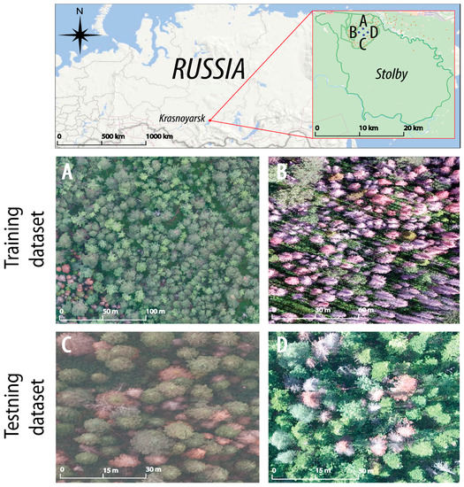
Figure 1.
Location of the four plots in the nature reserve “Stolby,” Krasnoyarsk city (Russia), where A, B plots are fragments from the orthophotos used to build the training dataset; and C, D plots are fragments from the orthophotos used to build the testing dataset used for external validation or independent testing.
A set of RGB images with ultra-high spatial resolution (≈5–10 cm/pix) were obtained for the research sites during multiple flights of the DJI Phantom 3 Pro quadcopter (with standard built-in camera) in July 2016 (plot A and C) and of the Yuneec Typhoon H hexacopter (with CGO3+ camera) in May 2016 (plot B) and August 2018 (plot D). Imagery for research plots A and C were recorded in cloudy weather conditions at 670 m (A) and 700 m (C) altitudes (120–150 m elevation above ground), plot B and D was surveyed in sunny weather at 120 m height. Default camera settings (auto white balance, ISO 100) were applied in all aerial shots. Image composites (orthophotomosaics) were created for each plot from a set of overlapping geolocated images (300–400 partially overlapping images per plot) using the Agisoft Photoscan Professional v1.4.0 (64-bit) software (www.agisoft.com, Agisoft LLC, St. Petersburg, Russia). This software provides photogrammetric and 3D-model reconstruction tools [31]. The data processing workflow in Photoscan consisted of the following steps: alignment of each image location, generation of dense point cloud (3D-model), creation of digital elevation model (DEM) and eventually production of a georeferenced orthophotomosaic (orthophotos or orthoimages from now). The workflow was run several times with varying settings in order to achieve better stich of images over the complex mountain landscape of the study sites. As a result, we got four orthophotos for each one of the four sites (A, B, C and D for 2016 and 2018).
5. Methods
As we have mentioned, our aim is to evaluate the possibilities of convolutional neural networks as a new approach to detect bark beetle outbreaks in fir trees in very high resolution imagery in fir and mixed forests. Thus, this section includes a definition of fir-tree damage categories (Section 5.1), describes the data pre-processing techniques we used for training the CNN models (Section 5.2), presents the classification model (Section 5.3) and finally presents the proposed detection technique especially designed for detecting bark beetle outbreaks in fir forests (Section 5.4).
5.1. Definition of Fir Trees Damage Categories
To define the categories of health status of fir trees, we followed the entomological approach by Krivets et al. [32], which differentiates six categories according to the level P. proximus invasion into the trunk and its influence on the canopy: I—healthy trees; II—weakened trees; III—heavily weakened trees; IV—dying trees; V—recently died trees; VI—old deadwood. Since the first, second and third categories can only be recognized in-situ by trunk signs that do not visibly translate into the crown, we reclassified them into four categories (skipping the second and the third one). Hence, the final categories in our classification were: a—completely healthy tree or recently attacked by beetles, b—tree colonized by beetles, c—recently died tree and d—deadwood (Figure 2).
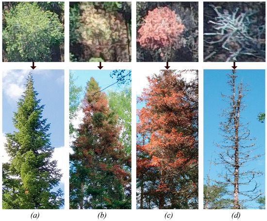
Figure 2.
Damage categories of Siberian fir trees used in this study (adapted from Krivets et al. [32]): (a) completely healthy tree or recently attacked by beetles, (b) tree colonized by beetles, (c) recently died tree and (d) deadwood. Top figures illustrate the vertical orthoimages corresponding to the bottom horizontal pictures.
5.2. Dataset Preprocessing and Data Augmentation Techniques of Sample patches for Training the CNN Models
The design of the training dataset is the key to the performance of a good CNN classification model. For labelling the training dataset, we identified 50 image patches containing 4 categories of trees. In particular, we built two different datasets:
- First, the dataset for training, validation and testing consisted in 50 manually sampled image-patches of single trees per each tree damage category, resulting in 200 image-patches from the plot A and B. To train the CNN model we used 80% of this selection. The remaining 20% of images were used for model internal validation.
- Second, the dataset for external testing or external validation consisted in 88 patch-images generated by our proposed detection technique from the areas C and D.
A summary of these two datasets is provided in Table 2.
Table 2.
Four fir tree categories training and testing datasets. Each image has 150 × 200-pixels.
The pre-processing method used for preparing the input UAV images is described in Table 1.
To improve the robustness and accuracy of the CNN classification models, we increased the volume of samples using data augmentation techniques. In particular, we increased the amount of sample patches for training the CNN models using the methods presented in Table 1.
The images of the training dataset were used for training the parameters of the neural network. The internal validation set is a set of examples used to tune the parameters of the neural network and determine a stopping point for the back-propagation algorithm. The testing dataset is a set of independent external examples used to assess or validate the performance of the final classification model.
5.3. Classification Model
A deep neural network was developed and trained on the prepared image samples to adapt its weights to the task of tree-damage recognition. To create a CNN and improve the quality of its training, we manually tuned the hyperparameters in the network. Several series of experiments were performed. For each experiment, the hyperparameters were altered and the consequent network’s operation quality change was estimated. The loss function, which should be minimized in the CNN (see Section 1), was established by a categorical cross-entropy loss between the input and the output classification of the images. The ADAM’s optimization was chosen among existing optimization algorithms since it was the most efficient one due to the possibility of initial calibration of the CNN. When exploring the effect of changing the learning rate parameter with the ADAM’s optimizer, the highest accuracy for CNN on the test data was achieved at a value of 0.0001. The total number of the network layers was determined by creating cascades of convolutional layers and a pooling layer. To assess the impact of the number of training epochs on the CNN accuracy, training was conducted and compared in the range from 1 to 50 epochs (see Section 6.2).
The overall architecture of the CNN (Table 3, Figure 3) consisted of six convolutional blocks (each includes one convolutional layer). Additionally, the first and third convolutional blocks included maximum pooling layers. At the top of the CNN, there are two fully connected layers and one output layer. The ReLU activation function was used in the last four convolutional blocks and the Softmax function for the output layer. In order to keep the overtraining of the network under control, we used the Dropout regularization method which reduced the complexity of the model, saving the number of its parameters low. It is very important to choose an appropriate regularization coefficient, so it was set to 0.25 after the second, fourth and fifth layers and it was set to 0.5 before the output layer. Our network with various activation functions is presented in Table 3.
Table 3.
The CNN network developed in this study, with different activation functions, where layers, output size and networks parameters are represented.
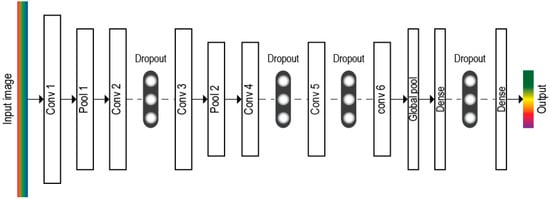
Figure 3.
The architecture of our CNN model of deep machine learning.
Consequently, our CNN model has the following form, presented in Figure 3.
5.4. Proposed Detection Process
We developed a candidate selection technique to find the potential regions in the test image that are more likely to be a tree. Then we analysed each one of these candidate regions using our CNN-classification model. The proposed candidate selection technique is a data processing algorithm that includes a sequence of the steps presented in the Table 4.
Table 4.
The proposed candidate selection technique in the test areas cropped from test areas C and D.
The output of this process are the candidate regions indicated by red bounding boxes in Figure 4. Finally, all the bounding boxes were analysed by the classification model.
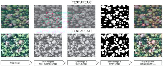
Figure 4.
Pre-processing consisted of the following steps: first, converting the three band image into one grey-scale band image (PAN); second, converting grey-scale band image into blurred image; third, converting the blurred image into a binary image based on a 100 over 256 digital value threshold; and fourth, detecting categories of trees on RGB images. The 48 candidate patches identified in test area C and 40 candidate patches identified in test area D are labelled with red contour in the right panel.
6. Results and Analysis
In this section, we will first describe the metrics used for the evaluation of the results of our proposed model, we will then show the performance of the training and internal test process (sites A and B) and finally we will show the results of the detection on two external test datasets of UAV images (sites C and D).
6.1. Evaluation Metrics
To evaluate and compare the results of the proposed CNN model with other CNN models, we used the performance metrics based on the confusion matrix. The confusion matrix is four by four (four categories) and contains the results of multi-class classifier (one class against the rest) in terms of number of true positive (TP) predictions, true negative (TN) predictions, false positive (FP) predictions and false negative (FN) predictions [34].
The main metrics we can extract from the matrix of confusion are: accuracy (1), precision (2), recall (3) and F-score (4). Accuracy is calculated as the total number of the correct predictions (TP + TN) divided by the total number of examples in the test set. Precision is calculated as the number of correct positive predictions (TP) divided by the total number of positive predictions (TP + FP). Recall is calculated as the number of correct positive predictions (TP) divided by the number of true positives and false negatives. F-score indicates the balance between precision and recall. The highest and best value of all these metrics is 1.0 and the worst is 0.0.
6.2. Evaluation of the Training Process and Comparison
To evaluate the training process of our new CNN, we used Python, Keras and TensorFlow framework with different pre-processing data augmentation techniques. Keras is a high-level API to ease the process of building and training deep learning models [35]. TensorFlow is open source software library for high performance numerical computation, which runs on various heterogeneous systems, including distributed graphics processing unit (GPU) clusters (Murray [36]). The used hardware environment in this study was Intel Xeon E5-2630v4 CPU accelerated with NVIDIA Titan Xp GPU as a platform for learning and testing.
The application of data augmentation techniques to the sample patches for training the CNN models resulted in the creation of 4400 image-patches from the first data subset, which had 200 patches (Section 5.2).
The maximum performance of our CNN model with augmented dataset was achieved at the 23th training epoch, providing an internal test accuracy of 99.7% and a minimum training loss lower than 0.01. After the 23th epoch, the validation loss was stabilized and the difference between the training and validation loss increased (Figure 5).
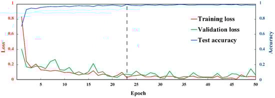
Figure 5.
Loss and accuracy for each epoch of the CNN model training with data augmentation.
For comparison with our CNN model, we have also tested on the same input data the most powerful CNN models such as Xception, VGG-16, VGG-19, ResNet-50, Inception-V3, InceptionResNet-V2, DenseNet-121, DenseNet-169 and DenseNet-201 (Jordan [37]). A brief explanation of each model is provided in Appendix B. We adapted the last layer of all these models to the 4 classes of our problem. The obtained results of all these models after few training epochs are shown in Appendix A (Table A1). As it can be seen from Table A1, all models provide high training accuracies.
6.3. External Test Detection Results
The confusion matrix of our CNN model in the four categories with data-augmentation are shown is Figure 6.
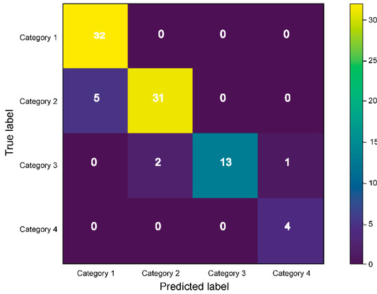
Figure 6.
Confusion matrix of the proposed CNN model with data augmentation on the candidate regions obtained from test areas C and D.
The results based on the confusion matrix of our CNN model on each category with and without data augmentation are shown in the Table 5.
Table 5.
The performance of our CNN model with and without data augmentation on the test set for each categories of trees. The performance is expressed in terms of true positives (TP), true negatives (TN), false positives (FP), false negatives (FN), precision, recall and F-score.
As it can be seen from Table 5, the trained CNN with data-augmentation provides the best test accuracy, recall and F1_score. The average accuracy, recall and F-score improved by 14.5%, 20.4% and 34.3% respectively. A comparison between the results obtained by our model and by more complex models with augmentation on the 88 candidate areas from images C and D is presented in Appendix A (Table A2). As it can be seen from this Table, although Xception, VGG16, VGG19, ResNet50, Inception V3, InceptionResNetV2, DenseNet121, DenseNet169 and DenseNet201 are powerful and computationally intensive models, our less computationally intensive architecture provides much better results in the damaged tree categories problem.
On the other hand, the proposed model with data-augmentation achieves high F1_score on damage class 1, 2, 3 and 4 with 92.75%, 89.86%, 89.66% and 88.89 respectively. This can be explained by the fact that the model correctly distinguishes the colour, shape and texture of each one of the four damage classes.
The results of the detection on the input test areas C and D are shown in Figure 7 and Figure 8. The red boxes present the selected areas produced by our candidate selection technique (see Section 5.4). Each red box has two numbers. The first number is the tree category estimated by the CNN model; C1, C2, C3 and C4 refer to the tree damage categories 1, 2, 3 and 4 respectively. The second number indicates the probability calculated by our classification CNN model. Actually, this probability indicates the level of confidence of the model.
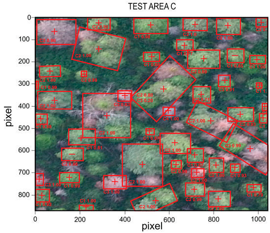
Figure 7.
Results of the detection of damaged tree categories on test area C. C1, C2, C3 and C4 indicate the estimated class by our CNN classification model together with the corresponding probability. The symbols “+” and “−” indicate respectively correct and incorrect class estimation by our model.

Figure 8.
Results of the detection of damaged tree categories on test area D. C1, C2, C3 and C4 indicate the estimated class by our CNN classification model together with the corresponding probability. The symbols “+” and “−” indicate respectively correct and incorrect class estimation by our model.
As it can be seen from Figure 7 and Figure 8, our model correctly recognizes the tree damage categories in most candidate regions (red boxes). In the few cases where the boxes include more than one tree crown, the model correctly predicts the existence of infected trees. Since the objective of this work is to detect infected trees, if a box has more than one tree and at least one of them is unhealthy and the model considers the entire box as unhealthy tree class, this answer is considered as valid answer for the purpose of finding unhealthy trees.
On the other hand, detecting individual trees in dense forests using only RGB bands information is a very complex task. In fact, previous studies (such as Mohan et al. [38]) that aimed to detect individual tree crowns in dense forests had to include several sources of data (high resolution images together with 3D LIDAR point cloud data), to achieve similar accuracies to our results. Actually, our results demonstrate that the proposed CNN based approach has a high potential and can be further improved in the future using more information, such as multispectral bands, NDVI or other spectral indices and 3D LIDAR data.
7. Conclusions
Damage to fir trees caused by the attacks of bark beetles is a major problem in the Taiga and Boreal Forests, particularly in Central Siberia of Russia. An efficient method for recognizing categories of tree damage using remote sensing imagery could substantially help as an early warning system that allows to eliminate fir trees colonized by the P. proximus beetle, to reduce its spread to new territories. The presented results are of great interest, both for scientific and practical purposes, since such work in the task of classifying categories of tree damage caused by beetle attacks to fir trees using CNN methods on UAV images has not yet been encountered. Recognizing the categories of damage to fir trees is a difficult task due to the fact that the forest canopy is very dense and diverse.
In this article, we developed a model based on CNNs to detect in RGB UAV images the damage to fir trees caused by bark beetles. Our network consists of six convolutional blocks. The network can recognize four damage categories in Siberian firs, from healthy to dead, with high prediction accuracy on images from different survey data. We have shown that our model provides better performance than the most powerful state-of-the-art CNN models, such as Xception, VGG, ResNet, Inception, InceptionResNet, DenseNet. We showed that data augmentation substantially increased the performance of our CNN model. Our model, trained with data augmentation, showed up to 98.77% accuracy for damage categories one, three and four. The second category may have the lowest recognition accuracy due to the fact that we had to merge three categories traditionally assessed in the field (weakened trees, heavily weakened trees and dying trees) into one category—trees colonized by the beetle, since it was not possible to visually observe any differences between these three categories in the UAV imagery.
Regarding alternative models, the VGG-16 model, on average, showed higher results, among other models considered in the paper. VGG-16 model recognized the first, second and fourth categories with an accuracy of 85.9%, 79.76 and 94.37%, respectively. Recognition of the third category with an accuracy higher than 88.89% is achieved by ResNet-50 model. The lowest accuracies were reached by InceptionResNet-V2.
In future works, we will focus on improving the segmentation of tree categories, introducing time series of data and trying to implement the three missing classes: weakened trees, heavily weakened trees and dying trees. It would also be interesting to explore if we can transfer our model to a new area with the same species and to other species, by only changing the last output layer in the network.
Author Contributions
A.S. and S.T. conceived and conducted the experiments, developed the CNN model and wrote the manuscript. A.R. made a survey of the research plots and a field exploration of the territory. A.S. prepared the training and testing datasets. D.A.-S. and A.R. made changes, revised and edited the first submitted version of the manuscript. A.S., S.T., D.A.-S., A.R., Y.M. and F.H. made changes, revised and edited the final version of the manuscript.
Funding
A.S. was supported by the grant of the Russian Science Foundation No. 16-11-00007. S.T. was supported by the Ramón y Cajal Programme (No. RYC-2015-18136). S.T. and F.H. received funding from the Spanish Ministry of Science and Technology under the project TIN2017-89517-P. D.A.-S. received support from project ECOPOTENTIAL, which received funding from the European Union Horizon 2020 Research and Innovation Programme under grant agreement No. 641762, from the European LIFE Project ADAPTAMED LIFE14 CCA/ES/000612 and from project 80NSSC18K0446 of the NASA’s Group on Earth Observations Work Programme 2016. A.R. was supported by the grant of the Russian Science Foundation No. 18-74-10048. Y. M. was supported by the grant of Russian Foundation for Basic Research No. 18-47-242002, Government of Krasnoyarsk Territory and Krasnoyarsk Regional Fund of Science.
Acknowledgments
We are very grateful to the reviewers for their valuable comments that helped to improve the paper. We appreciate the support of a vice-director of the “Stolby” State Nature Reserve, Anastasia Knorre. We also thank two Ph.D. students Egor Trukhanov and Anton Perunov from Siberian Federal University for their help in data acquisition (aerial photography from UAV) on two research plots in 2016 and raw imagery processing.
Conflicts of Interest
The authors declare no conflict of interest. The founding sponsors had no role in the design of the study; in the collection, analyses or interpretation of data; in the writing of the manuscript and in the decision to publish the results.
Abbreviations
The following abbreviations or terms are used in this manuscript:
| CNN | Convolutional neural networks |
| UAV | Unmanned aerial vehicle |
| P. proximus | Polygraphus proximus |
| RGB | Red, green, blue |
| ERS | Earth remote sensing |
| SVM | Support vector machine |
| RBF | Radial basis function |
| EPSG | Google Earth in European Petroleum Survey Group |
| OBIA | Object based image analysis |
| LDA | Linear discriminant analysis |
| PCA | Principal component analysis |
| RSI | Remote sensing indices |
| DJI | Dajiang Innovation Technology |
| QGIS | Quantum Geographic Information System |
| ADAM | ADAptive Moment estimation |
| ReLU | Rectified linear unit |
| TP | True positives |
| TN | True negatives |
| FP | False positives |
| FN | False negatives |
| API | Application programming interface |
| GPU | Graphics processing unit |
| CPU | Central processing unit |
Appendix A
Table A1.
Performance comparison of the training by proposed CNN model with other models.
Table A1.
Performance comparison of the training by proposed CNN model with other models.
| Model | Without Augmentation | With Augmentation | ||
|---|---|---|---|---|
| Loss | Accuracy | Loss | Accuracy | |
| Our CNN model | 0.05 | 1 | 0.001 | 1 |
| Xception | 0.3 | 0.89 | 0.002 | 1 |
| VGG-16 | 0.03 | 1 | 0.03 | 1 |
| VGG-19 | 0.07 | 1 | 0.01 | 0.99 |
| ResNet-50 + 4 | 0.21 | 0.94 | 0.01 | 1 |
| Inception-V3 + 4 | 0.34 | 0.89 | 0.003 | 1 |
| InceptionResNet-V2 + 4 | 0.13 | 0.94 | 0.04 | 0.99 |
| DenseNet-121 + 4 | 0.17 | 0.94 | 0.02 | 0.99 |
| DenseNet-169 + 4 | 0.08 | 1 | 0.004 | 0.99 |
| DenseNet-201 + 4 | 0.12 | 0.94 | 0.01 | 1 |
Table A2.
The results of testing alternative models for each class that were trained on data set with augmentation.
Table A2.
The results of testing alternative models for each class that were trained on data set with augmentation.
| Categories of Trees | TP | TN | FP | FN | Acc (%) | Precision (%) | Recall (%) | F-Score (%) |
|---|---|---|---|---|---|---|---|---|
| Xception | ||||||||
| 1 | 30 | 26 | 19 | 2 | 72.73 | 61.22 | 93.75 | 74.07 |
| 2 | 15 | 41 | 8 | 21 | 65.88 | 65.22 | 41.67 | 50.85 |
| 3 | 7 | 49 | 1 | 9 | 84.85 | 87.5 | 53.75 | 58.33 |
| 4 | 4 | 52 | 4 | 0 | 93.33 | 50 | 100 | 66.67 |
| VGG-16 | ||||||||
| 1 | 24 | 43 | 3 | 8 | 85.90 | 88.89 | 75 | 81.36 |
| 2 | 33 | 34 | 14 | 3 | 79.76 | 70.21 | 91.67 | 79.52 |
| 3 | 6 | 61 | 0 | 10 | 87.01 | 100 | 37.5 | 54.55 |
| 4 | 4 | 63 | 4 | 0 | 94.37 | 50 | 100 | 66.67 |
| VGG-19 | ||||||||
| 1 | 26 | 38 | 6 | 6 | 84.21 | 81.25 | 81.25 | 81.25 |
| 2 | 29 | 35 | 11 | 7 | 78.05 | 72.5 | 80.56 | 76.32 |
| 3 | 5 | 59 | 0 | 11 | 85.33 | 100 | 31.25 | 47.62 |
| 4 | 4 | 60 | 7 | 0 | 90.14 | 36.36 | 100 | 53.33 |
| ResNet-50 | ||||||||
| 1 | 32 | 32 | 16 | 0 | 80 | 66.67 | 100 | 80 |
| 2 | 20 | 44 | 1 | 16 | 79.01 | 95.24 | 55.56 | 70.18 |
| 3 | 9 | 55 | 1 | 7 | 88.89 | 90 | 56.25 | 69.23 |
| 4 | 3 | 61 | 6 | 1 | 90.14 | 33.33 | 75 | 46.15 |
| Inception-V3 | ||||||||
| 1 | 30 | 25 | 21 | 2 | 70.51 | 58.82 | 93.75 | 72.29 |
| 2 | 16 | 39 | 8 | 20 | 66.27 | 66.67 | 44.44 | 53.33 |
| 3 | 6 | 49 | 1 | 10 | 83.33 | 85.71 | 37.50 | 52.17 |
| 4 | 3 | 52 | 3 | 1 | 93.22 | 50 | 75 | 60 |
| InceptionResNet-V2 | ||||||||
| 1 | 23 | 27 | 14 | 9 | 68.49 | 62.16 | 71.88 | 66.67 |
| 2 | 18 | 32 | 11 | 18 | 63.29 | 62.07 | 50 | 55.38 |
| 3 | 6 | 44 | 6 | 10 | 75.76 | 50 | 37.5 | 42.86 |
| 4 | 3 | 47 | 7 | 1 | 86.21 | 30 | 75 | 42.86 |
| DenseNet-121 | ||||||||
| 1 | 26 | 33 | 10 | 6 | 78.67 | 72.22 | 81.25 | 76.47 |
| 2 | 24 | 35 | 8 | 12 | 74.68 | 75 | 66.67 | 70.59 |
| 3 | 6 | 53 | 1 | 10 | 84.29 | 85.71 | 37.50 | 52.17 |
| 4 | 3 | 56 | 10 | 1 | 84.29 | 23.08 | 75 | 35.29 |
| DenseNet-169 | ||||||||
| 1 | 32 | 26 | 21 | 0 | 73.42 | 60.38 | 100 | 75.29 |
| 2 | 15 | 43 | 5 | 21 | 69.05 | 75 | 41.67 | 53.57 |
| 3 | 8 | 50 | 1 | 8 | 86.57 | 88.89 | 50 | 64 |
| 4 | 3 | 55 | 3 | 1 | 93.55 | 50 | 75 | 60 |
| Dense Net-201 | ||||||||
| 1 | 32 | 22 | 22 | 0 | 71.05 | 59.26 | 100 | 74.42 |
| 2 | 15 | 39 | 7 | 21 | 65.85 | 68.18 | 41.67 | 51.72 |
| 3 | 4 | 50 | 1 | 12 | 80.6 | 80 | 25 | 38.1 |
| 4 | 3 | 51 | 4 | 1 | 91.53 | 42.86 | 75 | 54.55 |
Appendix B. Brief Description of the CNNs That Are Compared against the CNN Developed in This Work, That Is, VGG, ResNet, Inception-V3, InceptionResNet-V2, Xception and DenseNet
Visual Geometry Group (VGG) is a neural network architecture that has four variants, VGG-11, VGG-13, VGG-16 and VGG-19, where the number 13, 16 and 19 indicate the number of layers in the network. VGG-16 was designed by the University of Oxford to recognize objects in images. VGG-16 network is the 1st runner-up on the ImageNet Large Scale Visual Recognition Challenge (ILSVRC) comparison in 2014 with an obtained accuracy of 93.3% [39]. A distinctive feature of the architecture is a small convolution kernel of 3 × 3 pixels. The neural network architecture consists of two parts. The first part consists of alternating convolution cascades and a pooling layer: two convolution-convolution-pooling cascades and then three convolution-convolution-convolution-pooling cascades. On the pooling layer, Max Pooling is selected with a 2 × 2 square core. This part highlights the characteristic features in the image. The second part is responsible for the classification of the object in the image according to the features selected at the previous stage and includes three fully connected layers. Thus, the VGG-16 network receives images with a size of 224 × 224 pixels in three colour channels (red, green and blue) and the output represents the probability of belonging to a particular class in one hot encoding format. In our experiments, we compared our CNN to the following types of networks: VGG-16 and VGG-19.
ResNet was developed by Microsoft using residual learning for recognition, localization and detection of objects in images. It was the winner of the ILSVRC 2015 competition with 150 layers and the winner of Microsoft Common Objects in Context 2015 (MS COCO) detection and segmentation [40]. The authors of ResNet used the two-layer traversal approach and applied it on a large scale, which is considered as a small classifier in the network. The network also uses a bottleneck layer, which allows the reduction of the number of features in each layer, using a 1 × 1 pixel convolution with a lower yield of features and then a 3 × 3 pixel convolution layer and again a 1 × 1 pixel convolution layer with more features. The bottleneck layer reduces computational resources while preserves features combinations. The output layer is the pooling layer with the Softmax function. In our experiments, we compared our CNN to ResNet-50.
Inception-V3 is Google’s convolutional neural network for recognizing objects in an image. In December 2015, the third version of Inception was introduced with the inclusion of Batch-normalized Inception. Batch-normalization calculates the mean and standard deviation of all feature distribution maps in the output layer and then normalizes their responses with these values [20]. The last layer of the Inception network is the pooling layer with the Softmax function. To evaluate Inception-V3 on our data, we had to resize the input images from 150 × 200 to 299 × 299 pixels using cubic interpolation.
InceptionResNet-V2 is the union of two neural networks: Inception and ResNet. This allowed the authors to improve the accuracy of image classification. The idea of residual blocks was preserved from the Inception network and a combination of convolutional blocks from the ResNet network. Despite the fact that InceptionResNet-V2 demonstrates high accuracy compared to other existing models, it has two drawbacks: low speed and a high amount of memory used.
Xception was implemented in Keras by François Chollet and it is a modification of the Inception network (Chollet [41]). The network architecture is similar to ResNet-34 but the model and code is simpler than in Inception. A distinctive feature of the network architecture is SeparableConv, which is a modifiable, separable convolution that is located at the top of the network architecture. In the network there are residual (or shortcut/skip) connections, taken from the network ResNet. In addition, the network contains residual connections, which significantly increase the accuracy of classifying objects in images.
DenseNet is the result of the development of the ResNet network and is based on its residual blocks [21]. The basic idea is that connections have all the possible combinations within each block, which represents a gradient of more paths and the network becomes more resistant to learning. In our experiments, we compared our CNN to the following types of networks: DenseNet-121, DenseNet-169 and DenseNet-201.
References
- Bonan, G.B. Forests and climate change: Forcings, feedbacks, and the climate benefits of forests. Science 2008, 320, 1444–1449. [Google Scholar] [CrossRef]
- Hansen, M.C.; Potapov, P.V.; Moore, R.; Hancher, M.; Turubanova, S.A.; Tyukavina, A.; Thau, D.; Stehman, S.V.; Goetz, S.J.; Loveland, T.R.; et al. High-resolution global maps of 21st-century forest cover change. Science 2013, 342, 850–853. [Google Scholar] [CrossRef]
- Kuznetsov, V.; Sinev, S.; Yu, C.; Lvovsky, A. Key to Insects of the Russian Far East (in 6 Volumes). Volume 5. Trichoptera and Lepidoptera. Part 3. Available online: https://www.rfbr.ru /rffi/ru/books/o_66092 (accessed on 4 March 2019).
- Kerchev, I. Ecology of four-eyed fir bark beetle Polygraphus proximus Blandford (Coleoptera, Curculionidae, Scolytinae) in the west Siberian region of invasion. Rus. J. Biol. Invasions 2014, 5, 176–185. [Google Scholar] [CrossRef]
- Pashenova, N.V.; Kononov, A.V.; Ustyantsev, K.V.; Blinov, A.G.; Pertsovaya, A.A.; Baranchikov, Y.N. Ophiostomatoid fungi associated with the four-eyed fir bark beetle on the territory of russia. Rus. J. Biol. Invasions 2018, 9, 63–74. [Google Scholar] [CrossRef]
- Baranchikov, Y.; Akulov, E.; Astapenko, S. Bark beetle Polygraphus proximus: A new aggressive far eastern invader on Abies species in Siberia and European Russia. In Proceedings of the 21st U.S. Department of Agriculture Interagency Research Forum on Invasive Species, Annapolis, MD, USA, 12–15 January 2010. [Google Scholar]
- Helbig, M.; Wischnewski, K.; Kljun, N.; Chasmer, L.E.; Quinton, W.L.; Detto, M.; Sonnentag, O. Regional atmospheric cooling and wetting effect of permafrost thaw-induced boreal forest loss. Glob. Chang. Biol. 2016, 22, 4048–4066. [Google Scholar] [CrossRef]
- Ma, Z. The Effects of Climate Stability on Northern Temperate Forests. Ph.D. Thesis, Aarhus University, Aarhus, Denmark, March 2016. [Google Scholar]
- Lehmann, J.R.K.; Nieberding, F.; Prinz, T.; Knoth, C. Analysis of unmanned aerial system-based CIR images in forestry—A new perspective to monitor pest infestation levels. Forests 2015, 6, 594–612. [Google Scholar] [CrossRef]
- Li, W.; Fu, H.; Yu, L.; Cracknell, A. Deep learning based oil palm tree detection and counting for high-resolution remote sensing images. Remote Sens. 2016, 9, 22. [Google Scholar] [CrossRef]
- Guirado, E.; Tabik, S.; Alcaraz-Segura, D.; Cabello, J.; Herrera, F. Deep-learning versus OBIA for scattered shrub detection with google earth imagery: Ziziphus lotus as case study. Remote Sens. 2017, 9, 1220. [Google Scholar] [CrossRef]
- Baeta, R.; Nogueira, K.; Menotti, D.; dos Santos, J.A. Learning deep features on multiple scales for coffee crop recognition. In Proceedings of the 2017 30th SIBGRAPI Conference on Graphics, Patterns and Images (SIBGRAPI), Niteroi, Brazil, 17–20 October 2017; pp. 262–268. [Google Scholar]
- Kussul, N.; Lavreniuk, M.; Skakun, S.; Shelestov, A. Deep learning classification of land cover and crop types using remote sensing data. IEEE Geosci. Remote Sens. Lett. 2017, 14, 1–5. [Google Scholar] [CrossRef]
- Waser, L.T.; Küchler, M.; Jütte, K.; Stampfer, T. Evaluating the potential of worldview—2 data to classify tree species and different levels of ash mortality. Remote Sens. 2014, 6, 4515–4545. [Google Scholar] [CrossRef]
- Goodfellow, I.; Bengio, Y. Aaron Courville Deep Learning. MIT Press. Available online: https://mitpress.mit.edu/books/deep-learning (accessed on 4 March 2019).
- Tabik, S.; Peralta, D.; Herrera-Poyatos, A.; Herrera, F. A snapshot of image pre-processing for convolutional neural networks: Case study of MNIST. Int. J. Comput. Intell. Syst. 2017, 10, 555–568. [Google Scholar] [CrossRef]
- Deli, Z.; Bingqi, C.; Yunong, Y. Farmland scene classification based on convolutional neural network. In Proceedings of the 2016 International Conference on Cyberworlds (CW), Chongqing, China, 28–30 September 2016; pp. 159–162. [Google Scholar]
- Längkvist, M.; Kiselev, A.; Alirezaie, M.; Loutfi, A. Classification and segmentation of satellite orthoimagery using convolutional neural networks. Remote Sens. 2016, 8, 329. [Google Scholar] [CrossRef]
- Dyrmann, M.; Karstoft, H.; Midtiby, H. Plant species classification using deep convolutional neural network. Biosyst. Eng. 2016, 151, 72–80. [Google Scholar] [CrossRef]
- Razavi, S.; Yalcin, H. Using convolutional neural networks for plant classification. In Proceedings of the 25th Signal Processing and Communications Applications Conference (SIU), Antalya, Turkey, 15–18 May 2017; pp. 1–4. [Google Scholar]
- Dos Santos Ferreira, A.; Matte Freitas, D.; da Silva, G.; Pistori, H.; Folhes, M.T. Weed detection in soybean crops using ConvNets. Comput. Electron. Agric. 2017, 143, 314–324. [Google Scholar] [CrossRef]
- Onishi, M.; Ise, T. Automatic classification of trees using a UAV onboard camera and deep learning. arXiv, 2018; arXiv:1804.10390. [Google Scholar]
- Abdullah, H.; Darvishzadeh, R.; Skidmore, A.K.; Groen, T.A.; Heurich, M. European spruce bark beetle (Ips typographus, L.) green attack affects foliar reflectance and biochemical properties. Int. J. Appl. Earth Obs. Geoinf. 2018, 64, 199–209. [Google Scholar] [CrossRef]
- Heurich, M.; Ochs, T.; Andresen, T.; Schneider, T. Object-orientated image analysis for the semi-automatic detection of dead trees following a spruce bark beetle (Ips typographus) outbreak. Eur. J. For. Res. 2009, 129, 313–324. [Google Scholar] [CrossRef]
- Ortiz, S.M.; Breidenbach, J.; Kändler, G. Early detection of bark beetle green attack using terraSAR-X and rapideye data. Remote Sens. 2013, 5, 1912–1931. [Google Scholar] [CrossRef]
- Meddens, A.J.H.; Hicke, J.A.; Vierling, L.A.; Hudak, A.T. Evaluating methods to detect bark beetle-caused tree mortality using single-date and multi-date Landsat imagery. Remote Sens. Environ. 2013, 132, 49–58. [Google Scholar] [CrossRef]
- Näsi, R.; Honkavaara, E.; Lyytikäinen-Saarenmaa, P.; Blomqvist, M.; Litkey, P.; Hakala, T.; Viljanen, N.; Kantola, T.; Tanhuanpää, T.; Holopainen, M. Using UAV-based photogrammetry and hyperspectral imaging for mapping bark beetle damage at tree-level. Remote Sens. 2015, 7, 15467–15493. [Google Scholar] [CrossRef]
- Dash, J.P.; Watt, M.S.; Pearse, G.D.; Heaphy, M.; Dungey, H.S. Assessing very high resolution UAV imagery for monitoring forest health during a simulated disease outbreak. ISPRS J. Photogramm. Remote Sens. 2017, 131, 1–14. [Google Scholar] [CrossRef]
- Näsi, R.; Honkavaara, E.; Blomqvist, M.; Lyytikäinen-Saarenmaa, P.; Hakala, T.; Viljanen, N.; Kantola, T.; Holopainen, M. Remote sensing of bark beetle damage in urban forests at individual tree level using a novel hyperspectral camera from UAV and aircraft. Urban For. Urban Green. 2018, 30, 72–83. [Google Scholar] [CrossRef]
- Ryabovol, S.V. The Vegetetion of Krasnoyarsk. Modern Problems of Science and Education. Available online: https://www.science-education.ru/en/article/view?id=7582 (accessed on 1 March 2019).
- Agisoft PhotoScan User Manual—Professional Edition, Version 1.4. 127p. Available online: https://www.agisoft.com/pdf/photoscan-pro_1_4_en.pdf (accessed on 15 March 2019).
- Krivets, S.A.; Kerchev, I.A.; Bisirova, E.M.; Pashenova, N.V.; Demidko, D.A.; Petko, V.M.; Baranchikov, Y.N. Four-Eyed Fir Bark Beetle in Siberian Forests (Distribution, Biology, Ecology, Detection and Survey of Damaged Stands; UMIUM: Krasnoyarsk, Russia, 2015. [Google Scholar]
- Dawkins, P. Calculus III–Green’s Theorem. Available online: http://tutorial.math.lamar.edu/Classes/CalcIII/GreensTheorem.aspx (accessed on 23 November 2018).
- Basic Evaluation Measures from the Confusion Matrix. Classifier Evaluation with Imbalanced Datasets 2015. Available online: https://classeval.wordpress.com/introduction/basic-evaluation-measures/ (accessed on 15 March 2019).
- Keras Documentation. Available online: https://keras.io/ (accessed on 23 November 2018).
- Murray, C. Deep Learning CNN’s in Tensorflow with GPUs. Available online: https://hackernoon.com/deep-learning-cnns-in-tensorflow-with-gpus-cba6efe0acc2 (accessed on 23 November 2018).
- Jordan, J. Common Architectures in Convolutional Neural Networks. Available online: https://www.jeremyjordan.me/convnet-architectures/ (accessed on 2 August 2018).
- Mohan, M.; Silva, C.A.; Klauberg, C.; Jat, P.; Catts, G.; Cardil, A.; Hudak, A.T.; Dia, M. Individual tree detection from unmanned aerial vehicle (UAV) derived canopy height model in an open canopy mixed conifer forest. Forests 2017, 8, 340. [Google Scholar] [CrossRef]
- ImageNet Large Scale Visual Recognition Competition 2014 (ILSVRC2014). Available online: http://www.image-net.org/challenges/LSVRC/2014/results (accessed on 28 February 2019).
- COCO–Common Objects in Context. Available online: http://cocodataset.org/#home (accessed on 28 February 2019).
- Chollet, F. Xception: Deep learning with depthwise separable convolutions. arXiv, 2016; arXiv:1610.02357. [Google Scholar]


© 2019 by the authors. Licensee MDPI, Basel, Switzerland. This article is an open access article distributed under the terms and conditions of the Creative Commons Attribution (CC BY) license (http://creativecommons.org/licenses/by/4.0/).