Abstract
Past temporal gravity field solutions from the Gravity Recovery and Climate Experiment (GRACE), as well as current solutions from GRACE Follow-On, suffer from temporal aliasing errors due to undersampling of the signal to be recovered (e.g., hydrology), which arise in terms of stripes caused by the north–south observation direction. In this paper, we investigate the potential of the proposed mass variation observing system by high–low inter-satellite links (MOBILE) mission. We quantify the impact of instrument errors of the main sensors (inter-satellite link and accelerometer) and high-frequency tidal and non-tidal gravity signals on achievable performance of the temporal gravity field retrieval. The multi-directional observation geometry of the MOBILE concept with a strong dominance of the radial component result in a close-to-isotropic error behavior, and the retrieved gravity field solutions show reduced temporal aliasing errors of at least 30% for non-tidal, as well as tidal, mass variation signals compared to a low–low satellite pair configuration. The quality of the MOBILE range observations enables the application of extended alternative processing methods leading to further reduction of temporal aliasing errors. The results demonstrate that such a mission can help to get an improved understanding of different components of the Earth system.
1. Introduction
In times of a changing climate the need for innovative observation techniques for capturing geophysical processes in the Earth system becomes increasingly urgent. In this context, the observation of the temporal gravity field by satellites from space play an important role when investigating, e.g., rapid changes in the cryosphere, oceans, water cycle, and solid Earth processes on a global scale. For the determination of temporal gravity fields, in the last decade satellite missions such as GRACE [1] or Challenging Minisatellite Payload (CHAMP) [2,3] orbited around the globe and helped to get a better understanding of the Earth’s mass flux signals. CHAMP was based on high–low satellite-to-satellite tracking (SST) exploiting the Global Positioning System (GPS) [4] over a time span of 10 years. The accuracy of the CHAMP orbit information of 2–3 cm [5] derived from GPS allowed for resolving only the long wave range of the time varying gravity field, with spatial scales of ≈1000 km, e.g., Baur 2013 [6]. Analyzing the perturbed orbit of other Low Earth Orbiters (LEO), such as the Swarm satellites, allows for a similar performance [7]. The GRACE mission reached spatial scales of the temporal gravity field of ≈300 km and below due to a combination of K-band microwave low–low inter-satellite ranging between two identical satellites following each other in the same orbit at a distance of about 220 km with micrometer precision, and high–low GPS satellite-to-satellite tracking plus accelerometer observations. These missions improved our knowledge of water mass variations on the continents, in the oceans, and the atmosphere to a great extent. Additionally, the static gravity field retrieved from the Gravity field and steady-state Ocean Circulation Explorer (GOCE) [8] mission has improved our knowledge of the long-term static mass distribution, and has provided the physical reference surface of the geoid with centimeter precision with a spatial resolution down to 70–80 km.
The observation of the Earth’s gravity field will be continued by the GRACE Follow-On mission [9], which was successfully launched in May 2018. The instruments have been slightly modified compared to those used in GRACE, and additionally the GRACE Follow-On mission includes an inter-satellite laser ranging interferometer as a demonstrator [10], resulting in an increased accuracy of the SST observations to a few nanometers.
One of the main error contributions when observing the time variable gravity field results from geophysical signals with periods shorter than the temporal resolution of the satellite mission, as they alias into the solutions. Traditionally, the temporal resolution of the GRACE data products has been 30 days [1], leading to temporal aliasing effects due to non-tidal mass variations, especially atmospheric, oceanic, and hydrological signals having large amplitudes in the high-frequency range [11], as well as tidal signals with mainly semi-diurnal and diurnal periods. The temporal aliasing errors in GRACE appear in terms of striping effects, which are caused by the anisotropic error behavior resulting from along-track inter-satellite ranging. This type of error pattern also remains for the GRACE Follow-On mission because temporal aliasing errors clearly dominate the error budget of gravity field retrieval [12,13,14,15], while instrument errors of the laser interferometer only play a minor role in the total error budget.
In general, there are different approaches of how to deal with temporal aliasing errors: The gravity field solutions retrieved by GRACE are typically treated with de-striping and filtering techniques (e.g., References [16,17,18,19]), which are applied a posteriori in order to reduce the striping effects. A further de-aliasing method is proposed by Watkins et al. 2015 [20], where observations from GRACE are being processed using spherical cap mascons resulting in greater resolutions for smaller spatial regions. In the context of a Next Generation Gravity Field Mission (NGGM), various satellite constellations enabling a self-de-aliasing of high-frequency signals were investigated, such as the dual-tandem Bender-type mission [21], consisting of one near-polar pair and one inclined pair. Such a constellation allows the combination of two anisotropic measurements taken in different directions, which increases the isotropy of the combined system. A further concept is the pendulum formation where two satellites are on slightly shifted orbit planes in such a way that the line of sight between the satellites does not only contain along-track components, but also cross-track components [22]. Such innovative satellite constellations offer the application of improved gravity field processing methodologies in order to exploit the full potential of gravity field solutions with enhanced spatial and temporal resolution. Wiese et al. 2011 [23] proposed a method where low-resolution gravity field solutions are co-parameterized for short periods (e.g., daily) together with the long-term solutions (e.g., monthly) in order to mitigate the non-tidal high-frequency signals (especially atmosphere, ocean, and to some extent, also hydrology). A method to reduce tidal aliasing errors proposed by Hauk & Pail 2018 [24] aims at a co-parameterization of ocean tide parameters over time spans of several years, where the estimated tide model is used for de-aliasing during gravity field retrieval in a second processing step.
In this paper we pick up the point of new satellite constellations using an innovative observation concept of high-precision high–low inter-satellite ranging, which was proposed as the (MOBILE) mission [25] in response to European Space Agency (ESA)’s Earth Explorer 10 call. The observation geometry and the measuring principle of this satellite constellation are based on the Geodesy and Time Reference in Space (GETRIS) [26] concept describing a global space-borne infrastructure for data transfer, clock synchronization, and ranging, where gravity field recovery can be one of the first beneficiary applications of such an advanced geodetic space infrastructure.
In this study, we analyze the potential of the MOBILE mission qualitatively and quantitatively, and compare gravity field solutions with GRACE Follow-On-like solutions by means of full-scale numerical simulations. Furthermore, the potential of an extended processing method for the reduction of temporal aliasing is investigated for the MOBILE concept. In the following Section 2, the MOBILE observation configuration is described, while Section 3 gives an overview of the simulation environment including observation equations and stochastic modelling. In Section 4 the estimated gravity field solutions are analyzed and assessed. The main conclusions are summarized in Section 5, and in Section 6, a short outlook is given.
2. Mission Concept
2.1. Observation Geometry
In contrast to the past GRACE and the current GRACE Follow-On missions, which are mainly based on LEO satellites (several hundred km), the MOBILE minimum configuration consists of a constellation of two high and one low orbiting satellites. As done for GRACE and GRACE Follow-On, the main observable is the gravity-induced inter-satellite distance change, which is in case of MOBILE measured between medium orbiting satellites (MEO; several thousand km) and LEO satellites though. As a second gravity observation type, high-precision orbit positions based on Global Navigation Satellite System (GNSS) orbit determination are used. This idea of high-precision high–low tracking was first investigated by Hauk et al. 2017 [26] using the inter-satellite link technique as part of the payload on-board Galileo satellites of future generation in connection with LEO satellites, where the main error sources and the corresponding achievable performance were analyzed. Due to the fact that the MOBILE constellation presents a stand-alone concept without the need to place an additional payload on another space infrastructure, and the very large distance between the high- and the low orbiting satellites, which plays a crucial role in the framework of high-precision high-low tracking, dedicated MEO satellites were included in the concept. It should be emphasized that alternatively, a constellation of one MEO and two LEO satellites could be envisaged, which turns out to provide nearly the same performance as the proposed one, but might be more expensive due to the need to build and maintain at least two LEO satellites in orbit.
Figure 1 shows a schematic overview of the MOBILE satellite formation. The orbit parameters, which are used in the simulation environment to build up different satellite constellations, are listed in Table 1. The MEO satellites orbit at an altitude of about 10,150 km in the same orbital plane, separated by an 180-degree mean anomaly as alternating targets of the LEO satellites, in order to maximize the visibility and thus observation time. The LEO satellite is orbiting in an altitude of about 360 km. Both LEO and MEO satellites are flying in polar orbits in order to maintain a long-term stable formation (no relative drifts of the orbit planes). Additionally, two LEO satellites with near-polar orbits flying in an altitude of about 470 km with an inter-satellite distance of 200 km are set up in order to perform comparability studies between the MOBILE constellation and a GRACE Follow-On-like mission. All orbits have certain repeat cycles, after which the satellites reach the same position on Earth again in order to maintain a stable ground track pattern and related stable gravity model quality. The choice of the orbit height of the MEO satellites underlies three major constraints: (1) A high altitude of several thousand kilometers is necessary in order to ensure long observation periods and preferably measurements of multi-directional distance variations, with a strong dominance of the radial component, resulting in a close to isotropic error behavior of the retrieved gravity field solution (see Section 4). (2) The distance between a MEO–LEO pair must not be too large, because the larger the distance, the more difficult it is to fulfill the 1-µm accuracy requirement for the inter-satellite link established by a laser range interferometer (see Section 2.2). (3) The third constraint is driven by solar radiation belts encircling the Earth in which energetic charged particles are trapped inside the Earth’s magnetic field [27], which are of different intensities dependent on the solar cycle, altitude, and inclination of the satellite orbit. As a result, altitude ranges of several thousand kilometers below the chosen orbit height drop out. These conditions connected with the repeat orbit lead to an altitude of about 10,000 km for the MEO satellites.
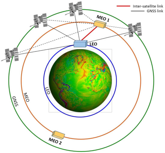
Figure 1.
MOBILE mission constellation: high-precision inter-satellite links between LEO and MEOs (red), micro-wave links from GNSS satellites to MEOs and LEO (black).

Table 1.
Orbit parameters for satellite constellations.
The high–low tracking concept enables a multi-directional observation geometry with differing elevation angles from 3° (assumed minimum elevation angle of visible MEOs observed by the LEO) up to a near-radial direction. However, due to the observation geometry of the MEO–LEO satellite pairs and the changing satellite links from one to the other MEO, data gaps arise for every satellite pair, leading to a non-continuous measurement time series of these pairs. For the simulated MOBILE constellation, this results in a ranging window maximum of 45 min, and a maximum data gap of 18 min. The separation of the two MEO satellites of 180-degree mean anomaly is chosen to keep the time period of the data gap as small as possible. In Figure 2, the LEO ground track of the MOBILE concept is displayed for 1 day together with the corresponding elevation angles.
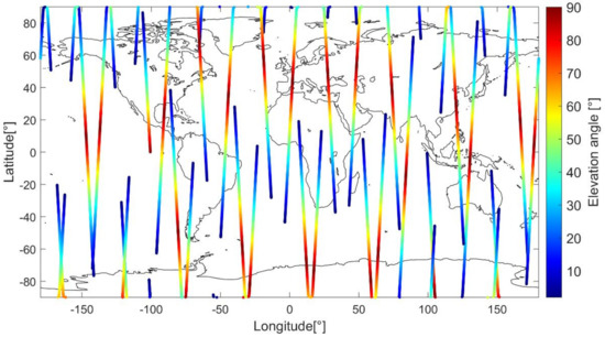
Figure 2.
One-day LEO ground track of the MOBILE mission constellation together with the elevation angle of visible MEOs observed by the LEO.
2.2. Instrumentation
The main observable in the MOBILE mission are range measurements from the LEO to the MEOs, where the MEOs are alternating targets. The ranging accuracy is on the micrometer level in order to be sensitive for gravitational forces and its changes on Earth. For distances of several thousand kilometers, a laser-based distance measurement system can reach such an accuracy. The laser range interferometer is placed at the LEO satellite, while the MEOs are equipped with passive reflectors or transponders. In case of the GRACE Follow-On mission, the measurement of inter-satellite ranges by laser range interferometry (LRI) has been successfully established. The link between the two satellites was generated with an active laser on one satellite, and a phase-locked amplifying transponder on the second spacecraft [10]. For the MOBILE concept, the laser ranging instrument needs to be adapted due to the very large distance and the relative motion of the LEO and MEO satellites. In contrast to the GRACE Follow-On, the large distance and the relative speed lead to a range of Doppler shifts of several GHz compared to a few MHz, which causes the need of a reference laser source with a larger range of reference frequencies and a faster phase-tracking capability than implemented for the GRACE Follow-On. The required parameters (<10 GHz range, <10 MHz/s tracking) are within the range of existing, space qualified reference lasers (e.g., the one used for the ATmospheric LIDar (ATLID) instrument on the Earth Clouds Aerosols and Radiation Explorer (CARE) mission) [28], but their compatibility with the needs of an interferometric instrument has to be the subject of further studies. Due to the relative motion of the LEO and MEO satellites, pointing tracking capabilities are required, which requires a modified link implementation. The LEO satellite is selected to play the active part in the tracking mechanism, while the partner satellites (MEOs) are equipped with passive retroreflectors. This type of laser tracking and ranging has been successfully performed for decades with active laser systems on the ground and passive retroreflectors on satellites in orbit (e.g., Laser Geodynamics Satellite (LAGEOS), Ball Lens In The Space (BLITS)) [29,30]. The scientific benefit of deploying a passive payload in space is the significantly increased mission duration when compared to complex active payloads. The main technological challenge in utilizing this setup for an LRI instrument is the need to achieve a sufficiently high level of retrieved power without the need for amplification between the two passes, ideally close to the 80 pW received by the GRACE Follow-On implementation, but at least to levels above ≈1 pW in order to allow phase tracking. The main design factors impacting the received power are the initial output power, the size of the retroreflector, and the size of the receiving telescope.
Satellite on-board sensors play an important role in the gravity field retrieval by influencing satellite observations due to correlated noise. In our study, the error assumptions used for the laser ranging instrument in the MOBILE concept are based on the time-series provided by Schäfer et al. 2013 [31], which originated in connection with ESA’s GETRIS study, and show micrometer ranging accuracy around 1 MHz. Due to simulation purposes, this time-series was adapted by means of cascaded second order Butterworth auto regressive moving average (ARMA) filter model. The spectral behavior of the LRI is shown in Figure 3 (light green curve) in terms of an amplitude spectral density (ASD). The relative distance measurement errors assumed for the low–low satellite pair are identical to those used in the frame of the ESA-Assessment of Satellite Constellations for Monitoring the Variations in Earth’s Gravity Field (SC4MGV) project [32], provided from the consultancy support of Thales Alenia Space Italia, and show a performance of about several 10 nanometers. The corresponding analytical noise model of the used laser interferometer is given by the ASD in terms of range-rates (Figure 3, light blue curve):
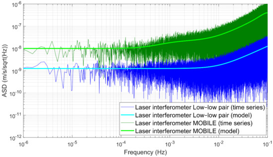
Figure 3.
Amplitude spectral density (ASD) of the relative distant measurement errors in terms of range-rates for the low–low pair formation (dark blue) and for MOBILE (dark green). The generation of the noise time-series was done by scaling the spectrum of normally distributed random time-series with their individual spectral model (light blue and light green curves).
The generation of all noise time-series was done by scaling the spectrum of normally distributed random time-series with their individual spectral model.
The non-gravitational forces are typically sensed by the on-board accelerometers located in the center-of-mass of the satellite. In case of the LEO satellites, the implementation of an accelerometer is absolutely necessary due to air drag as the main contributor. For the low–low pair a GRACE-like electrostatic accelerometer is assumed with two highly sensitive axes oriented in the flight direction (largest signal) and in the radial direction, and one low-sensitive axis in the cross-track direction (see Figure 4, blue and red curves). The accuracy level in terms of accelerations is derived by Iran Pour et al. 2015 [32], and is expressed by:
with denoting along-track, across-track, and (close to) the radial direction. Based on the heritage of previous gravity missions for MOBILE, we seek a resolution on the level of 10−11 m/s2, which is the same as assumed for the along-track and radial axes of the accelerometer on-board the low–low satellite pair, but ideally with the same performance in all three directions. Furthermore, the slope at frequencies from 10−3 Hz and lower is pressed down from 1/f2 for the low–low pair to 1/f for MOBILE. The performance of the relative acceleration measurement error is displayed in Figure 4 (green curve). While an accelerometer is mandatory for the MOBILE LEO satellite, for the MEOs, less stringent requirements might apply because of the substantially smaller amplitude of the signal and the fact that non-conservative forces can be modelled much more accurately in high altitudes. Also, the design of the MEO could be optimized for the high predictability of non-gravitational forces, e.g., by implementing very simple geometrical surfaces wherever radiative pressure is relevant. In spite of these facts, in the MOBILE concept, the implementation of accelerometers is proposed.
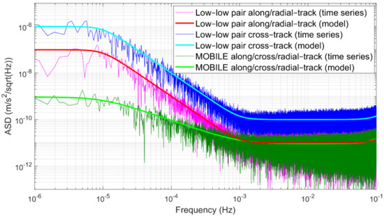
Figure 4.
Amplitude spectral density (ASD) of the relative acceleration measurement error in terms of accelerations for the low–low pair formation (dark blue and magenta) and for MOBILE (dark green). The generation of the noise time-series was done by scaling the spectrum of normally distributed random time-series with their individual spectral model (light blue, red, and light green curves).
Geo-location of satellite observations, as well as gravity retrieval, require highly accurate continuous orbit determination, making GNSS space receivers on all satellites obligatory. In our simulations, we assume an absolute kinematic positioning on a cm level. Using a laser ranging instrument as the main measurement system requires exact pointing of the tracking antenna in the order of 10 µrad or less, and therefore the implementation of systems for attitude determination and control. We assume star camera sensor errors for all satellites represented as rotation angles around the along-track (roll), cross-track (pitch), and radial (yaw) axes, expressed by the ASD of the following analytical noise models [32]:
In addition, for the MOBILE LEO satellite, a drag-reduction system needs to be implemented in order to maintain the orbit, and not to saturate the accelerometers due to non-gravitational accelerations. The MEO satellites will very likely require an electrical propulsion system to move to their target orbit from the lower separation altitude achievable with a low-cost launcher.
3. Simulation Environment
All simulations were executed with a full numerical mission simulator [33,34], which has already been successfully applied to recover satellite-only gravitational field models from GOCE data [35]. The simulation environment is based on numerical orbit integration, following a multistep method for the numerical integration according to Shampine & Gordon 1976 [36], which applies a modified divided difference form of the Adams predict-evaluate-correct-evaluate (PECE) formulas and local extrapolation. According to this method, the order and the step size are adjusted to control the local error per unit step in a generalized sense. The generation of “true” dynamic orbits and, subsequently, the “true” GNSS high–low SST and low–low laser ranging SST observations, is done by adding different force models according to the “true” world of Table 2. The impact of orbit errors on the gravity field processing is taken into account as well by propagating 1 cm white noise of the integrated orbit positions of each satellite. The resulting erroneous dynamic orbits serve as computational points for the reference values of the observations and enable the computation of the GNSS high–low SST observations in three directions. In order to ensure the accuracy of the inter-satellite link, error-free dynamic orbits are used for the reference values of the low–low SST observations from the laser interferometer system, which are expressed in terms of range-rates.
Table 2.
Force and noise models of the “true” and “reference” world used in the simulations.
The adopted gravity field approach is based on a modification of the integral equation approach from Schneider 1969 [37] where the orbit is divided into continuous short arcs of 6 h length, and the position vectors at the arc node points are set up as unknown parameters, which are estimated together with the gravity field coefficients. This technique has already been successfully applied in real data applications to recover satellite-only gravitational field models for CHAMP and GRACE [38] (ITSG-Grace2016) [39]. The functional model follows the typical formulation used for low–low SST missions like GRACE, which comprises a high–low SST and a low–low SST component. Position differences between two satellites are used for the computation of the reference values for the high–low SST part of the observation system, whereas the reference values for the low–low SST part are derived by projecting position and velocity differences between two satellites onto the line-of-sight, leading to the computation of inter-satellite range-rates. Table 2 gives an overview of the force and noise models used in the processing for the “true” and “reference” world. The static gravity field model is represented by the GOCO03s model, which is a satellite-only gravity field model based on GRACE, GOCE, and LAGEOS [40]. In order to simulate geophysical signals, ESA’s updated Earth system model [41] has been used, which contains the five main geophysical signal components atmosphere (A), ocean (O), hydrology (H), ice (I), and solid Earth (S) with a time resolution of six hours, linearly interpolated to the epochs. The Earth system model covers the time period 1995–2006, and contains plausible variability and trends in both low-degree coefficients and the global mean eustatic sea level. It depicts reasonable mass variability all over the globe at a wide range of frequencies including multi-year trends, year-to-year variability, and seasonal variability, even at very fine spatial scales, which is important for a realistic representation of spatial aliasing and leakage. The impact of ocean tide model errors is assessed by taking the difference of two tide models, EOT11a [42], and GOT4.7 [43].
The total stochastic model for the observations is approximated individually for both satellite formations by means of a cascade of digital Butterworth ARMA filters [44,45]. Filter coefficients are chosen in such a way that the cascade’s frequency response optimally matches the inverse of the amplitude spectrum of the previously generated pre-fit residuals. They are estimated as a result of the computation of the linearized normal equations, which include differences between the “true” (only the static GOCO03s gravity field model and sensor noise are included) and the reference observations (only the static GOCO03s gravity field model is included), such that the error sources from the sensors are considered exclusively. Assuming uncorrelated high–low and low–low SST observations, weighting matrices are set up for all observation components separately.
The goal is the retrieval of all spherical-harmonic (SH) coefficients up to a maximum SH degree of 100 from observations sampled every 5 seconds for the first 30 days of the year 2001. Due to the fact of non-linear observation equations, the “reference” observations are reduced from the “true” observations as a result of the linearization process. The gravity field parameters are estimated by solving full normal equations of a least squares system based on a standard Gauss–Markov model using weighted least squares with stochastic models in accordance with the simulated instrument noise levels. The resulting gravity field coefficients are analyzed and compared regarding quality and performance in terms of retrieval errors by removing a monthly average of the true mass transport model from the recovered signal.
4. Results
4.1. Gravity Field Retrieval Performance Due to Instrument Errors
At first the impact of the instrument errors on the gravity field retrieval were quantified. For this task, we performed simulations where each error source according to the assumptions described in Section 2.2 was treated individually. Figure 5 shows the gravity field retrieval performance in terms of equivalent water height (EWH) errors per SH degree per coefficient for the low–low pair constellation and the MOBILE concept. Furthermore, the results were quantified using global RMS values of the errors in the recovered signal expressed in terms of cm of EWH, listed in Table 3 (see part: instrument errors). If only white-noise positioning errors were considered (Figure 5, green curves), the gravity field retrieval performance mainly depended on the observation geometry. The comparison between both satellite concepts revealed strongly reduced retrieval errors for MOBILE, which benefited from multi-directional observations. In the case of accelerometer noise in combination with star camera errors (Figure 5, blue curves), the MOBILE constellation showed reduced error behavior compared to the low–low pair as well. This was mainly caused by the observation geometry, but also by the improved accelerometers (≈23%) with 3D capabilities to certain parts in the case of MOBILE. In contrast, the retrieval performance of the low–low pair benefits from the nanometer accuracy of the laser interferometer compared to the micrometer accuracy of MOBILE’s laser link sensor for the most part of the spectrum (>SH degree 10). This became evident when only laser interferometer noise was considered (Figure 5, red curves). However, in the very low degrees, the MOBILE concept performed better than GRACE, which was again owed to the fact of an improved observation geometry. When considering all instrument error sources together, the retrieval errors of the low–low satellite pair are dominated by the accelerometer plus star camera sensor performance, while for the MOBILE constellation, the laser link error was the dominating error source for SH degrees higher than 20, and the accelerometer plus star camera noise only dominated the spectrum in the lower degrees. These results led to the conclusion that the gravity field retrieval based on instrument error sources showed smaller errors below SH degree 40 for the MOBILE concept compared to the low–low pair, but increased errors in the higher frequency spectrum due to the lower accuracy of the laser interferometer.
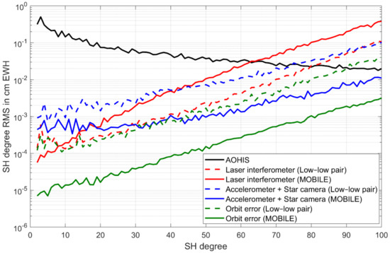
Figure 5.
Degree (error) standard deviations after 1 month of full AOHIS signal (black), low–low pair formation (dashed curves), and MOBILE constellation (continuous curves), when including only distance measurement errors (red), acceleration plus star camera errors (blue), and orbit errors (green).
Table 3.
Global RMS values in cm EWH for the low–low pair and MOBILE constellation considering different isolated error sources. RMS values are computed up to SH degree 100 for instrument errors, and up to SH degree 50 for temporal aliasing errors. Additionally, the global RMS value of the monthly averaged AOHIS and HIS signal is given (computed up to SH degree 50 and 100).
Next to the estimation of SH coefficients, we estimated their formal errors as well, shown in Figure 6. The noise of the different sensors in combination with the observation geometry reveal the performance of a specific satellite concept. In our case, they demonstrated the impact of the MOBILE high–low tracking concept by showing an almost uniform (isotropic) error spectrum and a high sensitivity in the sectorial coefficients (SH degree equal to SH order). In case of the low–low pair configuration especially, the sectorial coefficients were less well-determined than the zonal coefficients (SH order equal to zero). Figure 6b,d gave a closer view of the formal errors located in the long wavelength (low-degree) spectrum. The comparison between MOBILE and the low–low pair led to the assumption that the determination of the very low SH coefficients could be accomplished with a higher sensitivity through the MOBILE concept. In contrast to the observations in the along-track direction of the low–low pearl-string configuration, the multi-directional observations of the high–low tracking concept with a strong dominance of the radial component enabled an improved estimation of the very low SH coefficients. The close to radial observation geometry of MOBILE was comparable to satellite laser ranging (SLR) observations, showing superior performance in observing the very long wavelength gravity field variations, in particular the zonal SH coefficient of degree 2, which physically represented the Earth’s dynamic oblateness [46].
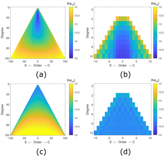
Figure 6.
Formal error triangle plots in up to SH degree and order 100 (a,c), and up to SH degree and order 10 (b,d), for the low–low pair formation (a,b), and the MOBILE constellation (c,d).
In order to make the effect of the different error spectra of both satellite concepts even more visible, spatial covariance functions were computed for a position at the equator and at 45° latitude (see Figure 7). They describe the correlation of the computation point with its neighborhood in the normal equation system due to the used stochastic model and the observation geometry. The spatial characteristics and the pattern of the covariances provide information about the spatial behavior of the retrieved signals. In our case, the figures show the typical stripes for the low–low tracking concept caused by the north–south observation direction that are known from the GRACE temporal gravity models, while the MOBILE concept exhibited an isotropic error structure at both latitudes.
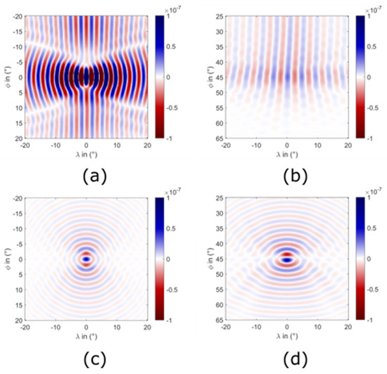
Figure 7.
Spatial covariance functions in m2 for the equator (a,c), and for 45° latitude (b,d), for the low–low pair formation (a,b), and the MOBILE constellation (c,d).
4.2. Temporal Gravity Field Retrieval
The retrieval of the temporal gravity field is dominated by temporal aliasing errors due to the undersampling of high frequency geophysical signals and imperfect de-aliasing models, which has already been shown by, e.g., References [47,48,49] for the GRACE mission. In order to analyze the impact of different time-varying mass signals on gravity field retrieval, we performed simulations by using signals that were subdivided into non-tidal AOHIS, HIS, and tidal signals, including the instrument errors described in Section 2.2. Figure 8 displays the corresponding retrieval errors for both satellite concepts. The results indicate that the errors with the highest signal amplitudes were related to AOHIS signals (Figure 8, red curves), and in particular to atmospheric and oceanic signals. Tidal aliasing effects played a key role in the total error budget as well (Figure 8, blue curves) by representing the highest aliasing errors next to non-tidal atmosphere and ocean aliasing errors. In this context it is important to mention that errors in ocean tide models are considered as one of the major sources of error in the determination of temporal gravity field models from GRACE data [50,51]. Our simulations show that the MOBILE configuration can reduce non-tidal aliasing errors (≈45%) as well as tidal aliasing errors (≈30%) over the whole spectrum significantly (see also Table 3, part: temporal aliasing errors). Despite the fact that for the high–low tracking concept the assumed arrangement of satellites causes incomplete data time series, the multi-directional observation geometry enables the sampling of time varying signals with reduced aliasing errors compared to the low–low pair configuration.
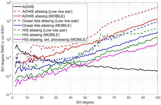
Figure 8.
Degree (error) standard deviations after 1 month of full AOHIS signal (black), low–low pair formation (dashed curves), and MOBILE constellation (continuous curves), when including only AOHIS signals + instrument errors (red), ocean tide signals + instrument errors (blue), HIS signals + instrument errors (green), and HIS signals + instrument errors using the extended processing method (magenta).
Usually high-frequency mass signals are a priori reduced based on atmosphere and ocean de-aliasing (AOD) products [52], and ocean tide de-aliasing models. The resulting temporal gravity field models thus contain mainly information on sub-seasonal, seasonal, and secular continental hydrological mass variations and ice mass variations on Earth [53,54], and solid Earth signals related to glacial isostatic adjustment (GIA), and co- and post-seismic gravity changes of big earthquakes. For the analysis of such mass flux signals we performed simulations by using only the HIS signal. The resulting gravity field retrieval errors (Figure 8, green curves) again revealed smaller aliasing effects for the MOBILE concept (≈60%), which is even better visible when looking at the spatial domain, shown in Figure 9. As already suggested by Figure 7, the retrieved HIS fields demonstrate, that the error pattern of MOBILE was much more homogeneous, and the typical striping of a low–low along-track ranging system is significantly reduced, particularly in the equatorial regions where the orbit ground tracks were less dense. This resulted in a clearly improved free representation of hydrological and ice mass signals for the MOBILE concept.
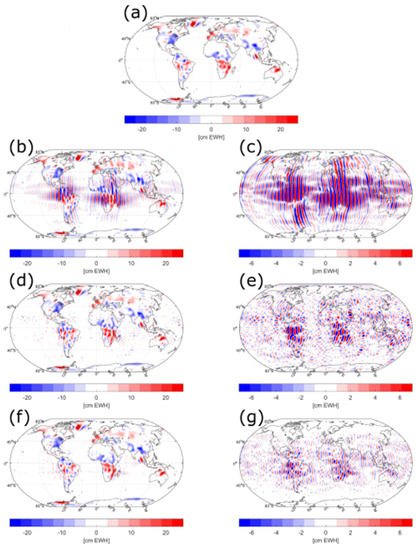
Figure 9.
Global grids of EWH (cm) up to SH degree and order 50 after 1 month. The grids show the true HIS signal (a), the recovered signal (b,d,f), and the differences of the true HIS signal and the recovered signal (c,e,g), for the low–low pair configuration (b,c), for the MOBILE concept (d,e), and for the MOBILE concept using the extended processing method (f,g).
The high quality of multi-directional observations of the high–low tracking concept allows the application of an extended alternative processing method first proposed by Wiese et al. 2011 [23], which enables the mitigation of temporal aliasing effects due to non-tidal time varying signals, as it was stated in Section 1. Wiese et al. 2011 [23] demonstrated the benefit of the co-parameterization of additional daily low degree and order gravity field coefficients for Bender-type satellite constellations. We investigated the potential of this methodology regarding the MOBILE concept by simulating a monthly solution while co-estimating daily gravity fields up to SH degree and order 10, including HIS signal plus instrument errors. The resulting retrieval errors are displayed in Figure 8 (magenta curve). They revealed an error reduction of about 40% compared to the nominal solution (green curve), which led to an increased spatial resolution of about SH degree 50 (≈400 km) instead of 40 (≈500 km). The corresponding spatial plot (Figure 9, f and g) shows a global reduced aliasing pattern, especially in higher latitudes. The comparison between the true HIS signal and the MOBILE recovered signal (nominal and extended processed) displayed in Figure 9 shows that the quality of the solutions could be improved to such a level that de-striping and smoothing the solutions was no longer necessary when examining signals to degree and order 50. Therefore, a possible loss of signal by a posteriori filtering of the gravity field solutions recovered by MOBILE could be avoided.
5. Conclusions
In this study, we investigated the gravity field retrieval performance of the novel and innovative MOBILE high–low satellite tracking concept and compared it with a low–low GRACE Follow-On-like configuration qualitatively and quantitatively. Based on full numerical simulations, gravity field parameters were estimated in terms of SH coefficients by solving a least-squares system by inverting full normal equations over a time span of 1 month. The most important error sources affecting the gravity field retrieval performance, key instruments on-board the satellites, as well as time varying mass flux signals, were included in order to assess their impact on gravity field retrieval for both mission concepts.
The results regarding the instrumental impact on the gravity field solution show that the performance of the MOBILE configuration was mainly limited by the assumed micrometer accuracy of the laser interferometer, especially in the short wavelength spectrum, while the performance in the lower wavelengths of the gravity field benefited from the multi-directional observation geometry and optimized 3D accelerometer. In contrast, the gravity field retrieval of the low–low pair constellation was limited mainly by the accelerometer, which predominated the nanometer accuracy of the assumed laser interferometer. The multi-directional observations of MOBILE mentioned above included a strong radial component and led to an almost uniform (isotropic) error spectrum, while the low–low tracking concept showed the typical stripes caused by the north–south observation direction. However, the high accuracy of the low–low satellite pair’s inter-satellite link led to an improved gravity field performance from SH degree 40 and higher compared to MOBILE, which performed better in the long wavelength spectrum where the largest amplitudes of time varying gravity field signals occurred.
The benefit of MOBILE’s multi-directional observation geometry arose when including tidal and non-tidal mass variation signals into the simulation process. The results revealed significantly reduced temporal aliasing errors in the recovered gravity field signal compared to the low–low tracking concept over the whole spectrum. In the case of the separate treatment of the HIS signal, the resulting gravity field error performance of MOBILE improved even by about 60%, and the application of an extended processing method to reduce temporal aliasing errors by co-estimation of daily gravity field parameters, led to a further reduction of retrieval errors of about 40%. Furthermore, the results show that the quality of recovered MOBILE gravity field solutions could make a treatment of such solutions using a posteriori filtering techniques obsolete.
The gravity field solutions retrieved using MOBILE can contribute to an improved understanding of different components of the Earth system, such as the estimation of continental water storage and freshwater fluxes, the quantification of large-scale flood and drought events and their monitoring and forecasting, or understanding the mass balance of ice sheets and larger glacier systems, just to name a few. The application of the extended processing method implied the co-parameterized gravity field parameters (which, in our case, are daily gravity fields) as a side product. These daily solutions with low spatial resolution could aid in improving atmospheric models, and possibly be beneficial to the oceanography community as well, as many of these short-term signals have large spatial scales.
6. Outlook
The gravity field solutions of the high–low tracking concept presented in this paper were based on the minimal configuration of MOBILE. On top of this scenario, the optional implementation of a third or fourth MEO satellite, but also a second LEO, could be considered to further increase the mission performance, but also significantly improve the temporal resolution. Due to the largely passive instrumentation of this mass transport mission, the function of the MEO satellites could be implemented as a backpack application of other MEO missions, such as the Galileo next-generation satellites, in order to extend and maintain the infrastructure for laser ranging payloads. Aside, one of the most important fields of research is the mitigation of temporal aliasing errors. In this context it is important to mention that aliasing effects due to imperfect ocean tide models represent one of the largest error sources in temporal gravity field retrieval. The capability of the multi-directional observations of MOBILE of co-parameterize tidal parameters over long time spans, as proposed in Reference [24], in order to improve current ocean tide models will be the subject of further study.
Author Contributions
Conceptualization, M.H. and R.P.; methodology, M.H.; software, M.H.; validation, M.H. and R.P.; formal analysis, M.H.; investigation, M.H.; resources, M.H. and R.P.; data curation, M.H.; writing—original draft preparation, M.H.; writing—review and editing, R.P.; visualization, M.H.; supervision, R.P.; project administration, R.P.; funding acquisition, R.P.
Funding
This research was funded by Deutsche Forschungsgemeinschaft (DFG), grant number, PA 1543/8-2 and the APC was funded by Institutional Open Access Program of the Technichal University of Munich (TUM).
Acknowledgments
A big part of the investigations presented in this paper was performed in the framework of the study “Two-way satellite tracking to provide a basis for gravity field mission scenarios—a simulation study with detailed error analysis II, ” Deutsche Forschungsgemeinschaft (DFG), Contract No. PA 1543/8-2 funded by DFG.
Conflicts of Interest
The authors declare no conflict of interest. The funders had no role in the design of the study; in the collection, analyses, or interpretation of data; in the writing of the manuscript, or in the decision to publish the results.
References
- Tapley, B.D.; Bettadpur, S.; Watkins, M.; Reigber, C. The gravity recovery and climate experiment experiment, mission overview and early results. Geophys. Res. Lett. 2004, 31, L09607. [Google Scholar] [CrossRef]
- Reigber, C.; Schwintzer, P.; Lühr, H. The CHAMP geopotential mission, in bollettino di geofisica teoretica ed applicata, 40/3-4, September–December 1999. In Proceedings of the Second Joint Meeting of the International Gravity and the International Geoid Commission, Trieste, Italy, 7–12 September 1998; pp. 285–289. [Google Scholar]
- Reigber, C.; Schwintzer, P.; Neumayer, K.H.; Barthelmes, F.; König, R.; Förste, C.; Balmino, G.; Biancale, R.; Lemoine, J.M.; Loyer, S.; et al. Earth gravity field model EIGEN-2. Adv. Space Res. 2003, 31, 1883–1888. [Google Scholar] [CrossRef]
- Xu, G. GPS. Theory, Algorithms and Applications; Springer: Berlin, Germany, 2003; ISBN 3-540-67812-3. [Google Scholar]
- Van den Ijssel, J.; Visser, P.; Patino Rodriguez, E. Champ precise orbit determination using GPS data. Adv. Space Res. 2003, 31, 1889–1895. [Google Scholar] [CrossRef]
- Baur, O. Greenland mass variation from time-variable gravity in the absence of GRACE. Geophys. Res. Lett. 2013, 40, 4289–4293. [Google Scholar] [CrossRef]
- Encarnação, J.T.; Arnold, D.; Bezděk, A.; Dahle, C.; Doornbos, E.; van den Ijssel, J.; Jäggi, A.; Mayer-Gürr, T.; Sebera, J.; Visser, P.; et al. Gravity field models derived from swarm GPS data. Earth Planets Space 2016, 68, 127. [Google Scholar] [CrossRef]
- Drinkwater, M.R.; Floberghagen, R.; Haagmans, R.; Muzi, D.; Popescu, A. GOCE: ESA’s first Earth explorer core mission. In Earth Gravity Field from Space—From Sensors to Earth Science, Space Sciences Series of ISSI; Kluwer Academic Publishers: Dordrecht, The Netherlands, 2003; Volume 18, pp. 419–432. ISBN 1-4020-1408-2. [Google Scholar]
- Flechtner, F.; Neumayer, K.H.; Dahle, C.; Dobslaw, H.; Fagiolini, E.; Raimondo, J.C.; Günter, A. What can be expected from the GRACE-FO laser ranging interferometer for Earth science applications? Surv. Geophys. 2016, 37, 453–470. [Google Scholar] [CrossRef]
- Sheard, B.S.; Heinzel, G.; Danzmann, K.; Shaddock, D.; Kilpstein, W.; Folkner, W. Intersatelite laser ranging instrument for the GRACE follow-on mission. J. Geod. 2012, 86, 1083–1095. [Google Scholar] [CrossRef]
- Murböck, M.; Pail, R. Reducing non-tidal aliasing effects by future gravity satellite formations. In Earth on the Edge: Science for a Sustainable Planet; Rizos, C., Willis, P., Eds.; International Association of Geodesy Symposia; Springer: Berlin/Heidelberg, Germany, 2014; Volume 139, pp. 407–412. ISBN 978-3-642-37222-3. [Google Scholar]
- Visser, P. Designing Earth gravity field missions for the future: A case study. In Gravity, Geoid and Earth Observation, International Association of Geodesy Symposia; Mertikas, S., Ed.; Springer-Verlag: Berlin/Heidelberg, Germany, 2010; Volume 135, pp. 131–138. [Google Scholar]
- Visser, P.; Sneeuw, N.; Reubelt, T.; Losch, M.; van Dam, T. Space-borne gravimetric satellite constellations and ocean tides: Aliasing effects. Geophys. J. Int. 2010, 181, 789–805. [Google Scholar] [CrossRef]
- Wiese, D.N.; Nerem, R.S.; Han, S.C. Expected improvements in determining continental hydrology, ice mass variations, ocean bottom pressure signals, and earthquakes using two pairs of dedicated satellites for temporal gravity recovery. J. Geophys. Res. 2011. [Google Scholar] [CrossRef]
- Daras, I.; Pail, R. Treatment of temporal aliasing effects in the context of next generation satellite gravimetry missions. J. Geophys. Res. 2017, 122, 7343–7362. [Google Scholar] [CrossRef]
- Swenson, S.; Wahr, J. Post-processing removal of correlated errors in GRACE data. Geophys. Res. Lett. 2006. [Google Scholar] [CrossRef]
- Kusche, J. Approximate decorrelation and non-isotropic smoothing of time-variable GRACE-type gravity field models. J. Geod. 2007, 81, 733–749. [Google Scholar] [CrossRef]
- Werth, S.; Güntner, A.; Schmidt, R.; Kusche, J. Evaluation of GRACE filter tools from a hydrological perspective. Geophys. J. Int. 2009, 179, 1499–1515. [Google Scholar] [CrossRef]
- Horvath, A. Retrieving Geophysical Signals from Current and Future Satellite Gravity Missions. Ph.D. Thesis, Technische Universität München, Munich, Germany, 2017. [Google Scholar]
- Watkins, M.; Wiese, D.N.; Yuan, D.N.; Boening, C.; Landerer, F.W. Improved methods for observing Earth’s time variable mass distribution with GRACE using spherical cap mascons. J. Geophys. Res. Solid Earth 2015, 120, 2648–2671. [Google Scholar] [CrossRef]
- Bender, P.L.; Wiese, D.N.; Nerem, R.S. A possible dual-GRACE mission with 90 degree and 63 degree inclination orbits. In Proceedings of the Third International Symposium on Formation Flying, Missions and Technologies, Noordwijk, The Netherlands, 23–25 April 2008; pp. 1–6. [Google Scholar]
- Sharifi, M.A.; Sneeuw, N.; Keller, W. Gravity recovery capability of four generic satellite formations. In Proceedings of the 1st International Symposium of the International Gravity Field Sevice “Gravity Field of the Earth”, Istanbul, Turkey, 28 August–1 September 2007. [Google Scholar]
- Wiese, D.N.; Visser, P.; Nerem, R.S. Estimating low resolution gravity fields at short time intervals to reduce temporal aliasing errors. Adv. Space Res. 2011, 48, 1094–1107. [Google Scholar] [CrossRef]
- Hauk, M.; Pail, R. Treatment of ocean tide aliasing in the context of a next generation gravity field mission. Geophys. J. Int. 2018, 214, 345–365. [Google Scholar] [CrossRef]
- Pail, R.; Bamber, J.; Biancale, R.; Bingham, R.; Braitenberg, C.; Cazenave, A.; Eicker, A.; Flechtner, F.; Gruber, T.; Güntner, A.; et al. Mass variation observing system by high low inter-satellite links (MOBILE)—A mission proposal for ESA Earth Explorer 10. In Proceedings of the 20th EGU General Assembly, EGU2018, Vienna, Austria, 4–13 April 2018. [Google Scholar]
- Hauk, M.; Schlicht, A.; Pail, R.; Murböck, M. Gravity field recovery in the framework of a Geodesy and Time Reference in Space (GETRIS). Adv. Space Res. 2017, 59, 2032–2047. [Google Scholar] [CrossRef]
- Van Allen, J.A. Discovery of the magnetosphere. In History of Geophysics; Gillmor, C.S., Spreiter, J.R., Eds.; American Geophysical Union: Washington, DC, USA, 1997; Vol. 7, pp. 235–251. ISBN 978-0875902883. [Google Scholar]
- Illingworth, A.J.; Barker, H.W.; Beljaars, A.; Ceccaldi, M.; Chepfer, H.; Cole, J.; Delanoë, J.; Domenech, C.; Donovan, D.P.; Fukuda, S.; et al. The Earthcare satellite: The next step forward in global measurements of clouds, aerosols, precipitation and radiation. Bull. Am. Meteorol. Soc. 2015, 96, 1311–1332. [Google Scholar] [CrossRef]
- Spencer, R.L. Lageos—A geodynamics tool in the making. J. Geol. Educ. 1977, 25, 38–42. [Google Scholar] [CrossRef]
- Kucharski, D.; Kirchner, G.; Lim, H.C.; Koidl, F. Optical response of nanosatellite BLITS measured by the Graz 2 kHz SLR system. Adv. Space Res. 2011, 48, 1335–1340. [Google Scholar] [CrossRef]
- Schäfer, W.; Flechtner, F.; Nothnagel, A.; Bauch, A.; Hugentobler, U. Geodetic Time Reference in Space (GETRIS); ESA Study AO/1-6311/2010/F/WE Final Report GETRIS-TIM-FR-0001; 2013. [Google Scholar]
- Iran Pour, S.; Reubelt, T.; Sneeuw, N.; Daras, I.; Murböck, M.; Gruber, T.; Pail, R.; Weigelt, M.; van Dam, T.; Visser, P.; et al. Assessment of Satellite Constellations for Monitoring the Variations in Earth Gravity Field—SC4MGV; ESA—ESTEC Contract No. AO/1-7317/12/NL/AF, Final Report; 2015. [Google Scholar]
- Daras, I.; Pail, R.; Murböck, M.; Yi, W. Gravity field processing with enhanced numerical precision for LL-SST missions. J. Geod. 2015, 89, 99–110. [Google Scholar] [CrossRef]
- Daras, I. Gravity Field Processing Towards Future LL-SST Satellite Missions. Ph.D. Thesis, Technische Universität München, Munich, Germany, 2016; pp. 23–39. [Google Scholar]
- Yi, W. The Earth’s Gravitational Field from GOCE. Ph.D. Thesis, Centre of Geodetic Earth System Research, Munich, Germany, 2012. [Google Scholar]
- Shampine, L.F.; Gordon, M.K. Computer Solution of Ordinary Differential Equations: The Initial Value Problem; W.H. Freeman: San Francisco, CA, USA, 1975. [Google Scholar]
- Schneider, M. Outline of a general orbit determination method. In Space Research IX, Proceedings of the Open Meetings of Working Groups (OMWG) on Physical Sciences of the 11th Plenary Meeting of the Committee on Space Research (COSPAR), Tokyo, Japan; Mitteilungen aus dem Institut für Astronomische und Physikalische Geodäsie, Nr. 51; Champion, K.S.W., Smith, P.A., Smith-Rose, R.L., Eds.; North Holland Publ. Company: Amsterdam, The Netherlands, 1969; pp. 37–40. [Google Scholar]
- Mayer-Gürr, T. Gravitationsfeldbestimmung aus der Analyse Kurzer Bahnbögen am Beispiel der Satellitenmissionen CHAMP und GRACE. Ph.D. Thesis, Rheinische Friedrich-Wilhelms-Universität zu Bonn, Bonn, Germany, 2006. [Google Scholar]
- Mayer-Gürr, T.; Jäggi, A.; Meyer, U.; Yoomin, J.; Susnik, A.; Weigelt, M.; van Dam, T.; Flechtner, F.; Gruber, C.; Günter, A.; et al. European gravity service for improved emergency management—Status and project highlights. In Proceedings of the EGU General Assembly, EGU 2016, Vienna, Austria, 17–22 April 2016. [Google Scholar]
- Mayer-Gürr, T.; Rieser, D.; Höck, E.; Brockmann, J.M.; Schuh, W.D.; Krasbutter, I.; Kusche, J.; Maier, S.; Krauss, S.; Hausleitner, W.; et al. The new combined satellite only model GOCO03s. In Proceedings of the IAG Symposium Gravity, Geoid and Height Systems, Venice, Italy, 9–12 October 2012. [Google Scholar]
- Dobslaw, H.; Bergmann-Wolf, I.; Dill, R.; Forootan, E.; Klemann, V.; Kusche, J.; Sasgen, I. The updated ESA Earth system model for future gravity mission simulation studies. J. Geod. 2015, 89, 505–513. [Google Scholar] [CrossRef]
- Savcenko, R.; Bosch, W. EOT11a-Empirical Ocean Tide Model from Multi-Mission Satellite Altimetry; DGFI Report No. 89; Deutsches Geodätisches Forschungsinstitut: München, Germany, 2012. [Google Scholar]
- Ray, R. A Global Ocean Tide Model from Topex/Poseidon Altimetry: Got99.2; NASA Technical Memorandum 209478; Goddard Space Flight Center: Greenbelt, Maryland, 1999. [Google Scholar]
- Siemes, C. Digital Filtering Algorithms for Decorrelation within Large Least Square Problems. Ph.D. Thesis, University of Bonn, Bonn, Germany, 2008. [Google Scholar]
- Pail, R.; Bruinsma, S.; Migliaccio, F.; Förste, C.; Goiginger, H.; Schuh, W.D.; Höck, E.; Reguzzoni, M.; Brockmann, J.M.; Abrikosov, O.; et al. First GOCE gravity field models derived by three different approaches. J. Geod. 2011, 85, 819–843. [Google Scholar] [CrossRef]
- Cheng, M.K.; Tapley, B.D. Seasonal variations in low degree zonal harmonics of the Earth’s gravity field from satellite laser ranging observation. J. Geophys. Res. 1999, 104, 2667–2681. [Google Scholar] [CrossRef]
- Zenner, L.; Gruber, T.; Jaeggi, A.; Beutler, G. Propagation of atmospheric model errors to gravity potential harmonics-impact on GRACE de-aliasing. Geophys. J. Int. 2010, 182, 797–807. [Google Scholar] [CrossRef]
- Han, S.; Jekeli, C.; Shum, C. Time-variable aliasing effects of ocean tides, atmosphere, and continental water mass on monthly mean GRACE gravity field. J. Geophys. Res. 2004, 109, B04403. [Google Scholar] [CrossRef]
- Thompson, P.; Bettadpur, S.; Tapley, B.D. Impact of short period, non-tidal, temporal mass variability on GRACE gravity estimates. Geophys. Res. Lett. 2004, 31, L06619. [Google Scholar] [CrossRef]
- Knudsen, P.; Andersen, O. Correcting GRACE gravity fields for ocean tide effects. Geophys. Res. Lett. 2002, 29, 1178. [Google Scholar] [CrossRef]
- Seo, K.W.; Wilson, C.R.; Han, S.C.; Waliser, D.E. Gravity recovery and climate experiment (GRACE) alias error from ocean tides. J. Geophys. Res. 2008, 113, B03405. [Google Scholar] [CrossRef]
- Flechtner, F. AOD1b Product Description Document for Product Releases 01 to 04; GRACE 327-750; GeoForschungszentrum Potsdam: Potsdam, Germany, 2007. [Google Scholar]
- Tiwari, V.M.; Wahr, J.; Swenson, S. Dwindling groundwater resources in northern India, from satellite gravity observations. Geophys. Res. Lett. 2009, 36, L18401. [Google Scholar] [CrossRef]
- Velicogna, I.; Sutterley, T.C.; van den Broeke, M.R. Regional acceleration in ice mass loss from Greenland and Antarctica using GRACE time-variable gravity data. Geophys. Res. Lett. 2014, 41, 8130–8137. [Google Scholar] [CrossRef]
© 2019 by the authors. Licensee MDPI, Basel, Switzerland. This article is an open access article distributed under the terms and conditions of the Creative Commons Attribution (CC BY) license (http://creativecommons.org/licenses/by/4.0/).