Article

Automatic Ship Detection Based on RetinaNet Using Multi-Resolution Gaofen-3 Imagery

1
Key Laboratory of Digital Earth Science, Institute of Remote Sensing and Digital Earth, Chinese Academy of Sciences, Beijing 100094, China
2
College of Resources and Environment, University of Chinese Academy of Sciences, Beijing 100049, China
*
Author to whom correspondence should be addressed.
Remote Sens. 2019, 11(5), 531; https://doi.org/10.3390/rs11050531
Submission received: 19 January 2019 / Revised: 22 February 2019 / Accepted: 27 February 2019 / Published: 5 March 2019
(This article belongs to the Section Ocean Remote Sensing)

Abstract

:
Independent of daylight and weather conditions, synthetic aperture radar (SAR) imagery is widely applied to detect ships in marine surveillance. The shapes of ships are multi-scale in SAR imagery due to multi-resolution imaging modes and their various shapes. Conventional ship detection methods are highly dependent on the statistical models of sea clutter or the extracted features, and their robustness need to be strengthened. Being an automatic learning representation, the RetinaNet object detector, one kind of deep learning model, is proposed to crack this obstacle. Firstly, feature pyramid networks (FPN) are used to extract multi-scale features for both ship classification and location. Then, focal loss is used to address the class imbalance and to increase the importance of the hard examples during training. There are 86 scenes of Chinese Gaofen-3 Imagery at four resolutions, i.e., 3 m, 5 m, 8 m, and 10 m, used to evaluate our approach. Two Gaofen-3 images and one Constellation of Small Satellite for Mediterranean basin Observation (Cosmo-SkyMed) image are used to evaluate the robustness. The experimental results reveal that (1) RetinaNet not only can efficiently detect multi-scale ships but also has a high detection accuracy; (2) compared with other object detectors, RetinaNet achieves more than a 96% mean average precision (mAP). These results demonstrate the effectiveness of our proposed method.

1. Introduction

Synthetic aperture radar (SAR) operates in all weathers and during day and night, and SAR imagery is widely used for ship detection in marine monitoring, such as for transportation safety and fishing law enforcement [1,2,3,4]. With the launch of SAR satellites, such as China’s Gaofen-3 in August of 2016, Japan’s Advanced Land Observing Satellite 2 (ALOS-2) in May of 2014, and Sentinel-1 of the European Space Agency in April of 2014, numerous SAR images are available to dynamically monitor the ocean. Traditional ship detection approaches are mainly constant false alarm rates (CFAR) based on the statistical distributions of the sea clutter [5,6,7,8] and the extracted features based [9,10,11,12]. These two methods are highly dependent on the distributions or features predefined by humans [3,9,13,14], degrading the performance of ship detection for a new SAR imagery [9,14]. Therefore, they may be less robust.
Being able to automatically learn representation [15,16], object detectors in deep learning have achieved top performance with regards to detection accuracy and speed, such as Faster regions with convolutional neural networks (R-CNN) [17], single shot multibox detector (SSD) [18], You Only Look Once (YOLO) [19,20], and RetinaNet [21]. These detectors can be divided into one-stage detectors and two-stage detectors [21]. Two-stage detectors are usually slower than one-stage detectors because of the generation of the candidate object location using an external module and because of the higher detection accuracy due to the consideration of the hard examples [21]. Here, the hard examples are the examples poorly predicted by the model. Recently, Reference [21] embraces the advantages of one-stage detectors and introduces the focal loss to help these models to have not only a fast speed but also a high detection accuracy, such as RetinaNet and YOLO-V3 [19]. Therefore, object detectors in deep learning, such as Faster RCNN and SSD, have been adapted to address ship detection in SAR images [1,2,3,22]. Kang et al. [2] used the faster RCNN method to obtain the initial ship detection results and then applied (constant false alarm rate) CFAR to obtain the final results. Li et al. [22] proposed the use of feature fusion, transfer learning, hard negative mining, and other implementation details to improve the performance of Faster R-CNN. Wang et al. [3] combined transfer learning with a single shot multibox detector for the detection of ships, with the consideration of both detection accuracy and speed. Kang et al. [
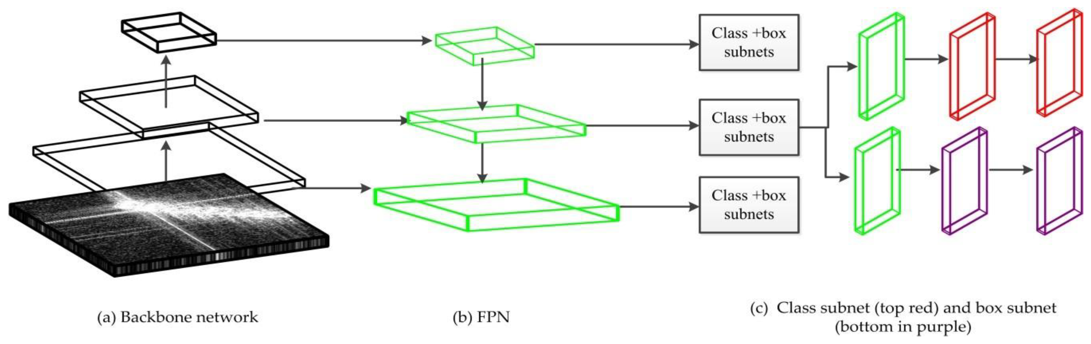
1] proposed a region-based convolutional neural network with contextual information and multilayer features for ship detection and combined the low-level high-resolution features and high-level semantic features to improve the detection accuracy and to remove some errors based on contextual information. The methods are mainly modified from Faster RCNN and SSD, which do not explore the state-of-the-art RetinaNet. There are two main building blocks in RetinaNet: feature pyramid networks (FPN) [23] and focal loss. The former is used to extract multi-scale features for both ship classification and location. The latter is used to address the class imbalance and to increase the importance of the hard examples.
Targets on SAR imagery are sensitive to pose and configuration [8,24]. For ships, their shapes are multi-scale. The first reason is that, due to the influence of various resolutions, the shapes of the same ship are multi-scale, and the second is that vessels with various shapes display differently in the same resolution SAR imagery. Therefore, it is necessary to consider the variance of ship scales. Currently, there are several studies to deal with this [1,2,3,4,9,22,25]. Except in Reference [4], the datasets in the papers of Reference [9,22,25] are limited, or some only provide samples for a single-resolution SAR image ship detection [1,2,3]. The China Gaofen-3 satellite, successfully launched in August 2016, could provide data support for long-term scientific research. Therefore, 86 scenes of Chinese Gaofen-3 Imagery at four resolutions, i.e., 3 m, 5 m, 8 m, and 10 m, are studied experimentally in this paper.
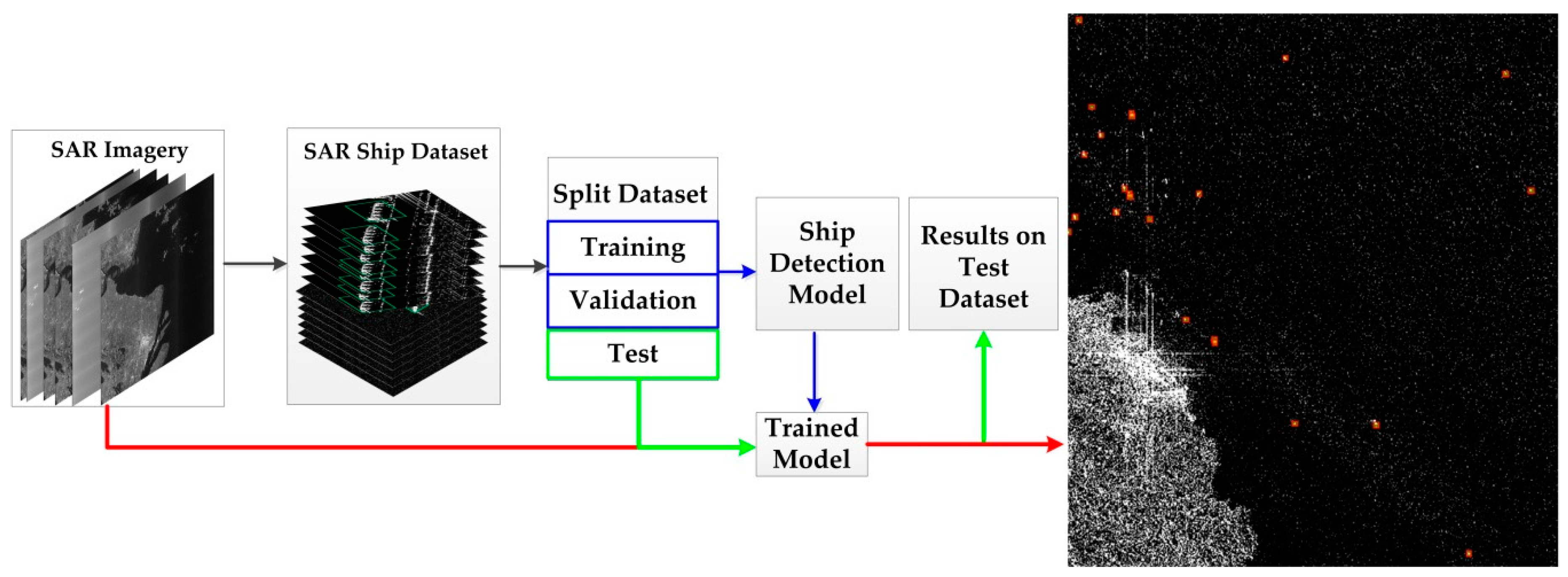
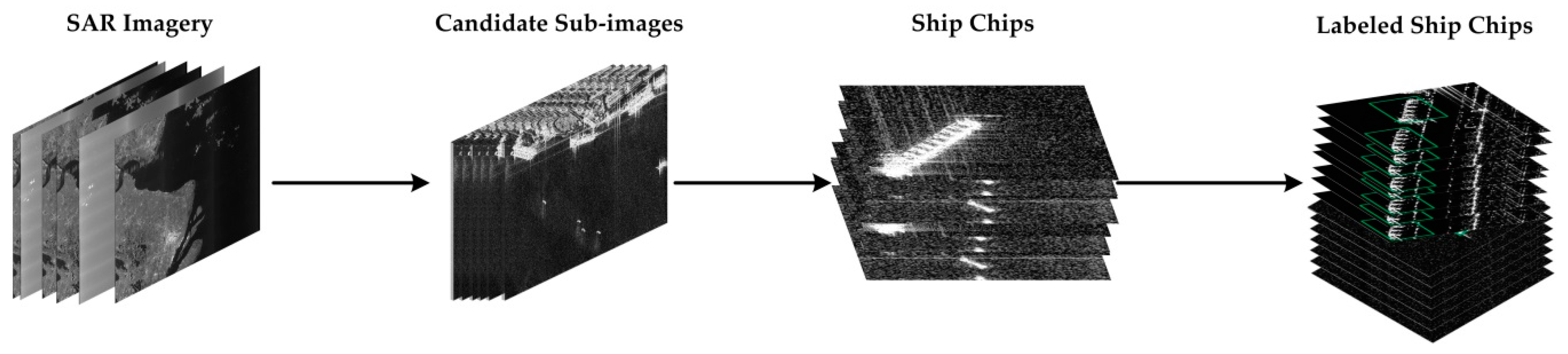
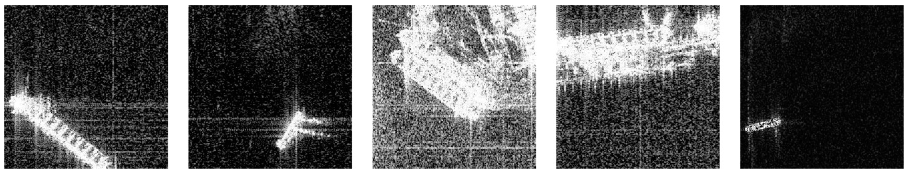
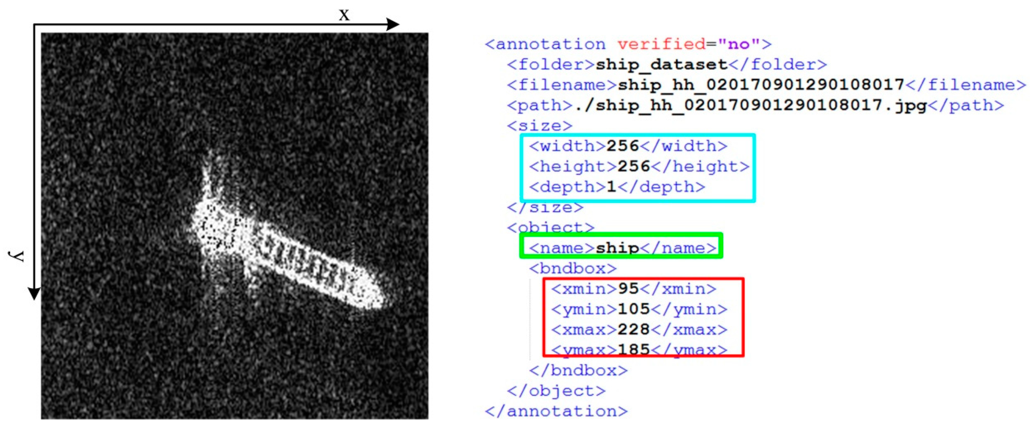
One important reason restricting the adaption of object detectors in deep learning to ship detection is the scarce dataset. To relieve this predicament, 9974 SAR ship chips with 256 pixels in both range and azimuth are constructed. They are used to evaluate our methods. They can be used to boost the application of computer vision techniques, especially object detectors in deep learning to ship detection in SAR images, and can also facilitate the emergence of more advanced object detectors with the consideration of SAR characteristics, such as the speckle noise.
Based on the above analysis, RetinaNet is adapted to address ship detection in this paper. To better evaluate our proposed method, two Gaofen-3 images and one CosMo-SkyMed image are used to test the robustness. The main contributions in this paper are as follows:
  • A large volume of the ship chips in multi-resolution SAR images is constructed with the aim to exploit the benefits of object detectors in deep learning. We believe this dataset will boost the application of computer vision techniques to SAR application.
  • A state-of-the-art performance object detector, i.e., RetinaNet, is applied to the ship detection in multi-resolution Gaofen-3 SAR imagery. It achieves more than a 96% mean average precision (mAP) and ranks first compared with the other three models.
The organization of this paper is as follows. Section 2 relates to the background of RetinaNet and the proposed method. Section 3 reports on the experiments, including the dataset and experimental analysis. Section 4 and Section 5 come to a discussion and conclusion.

2. Materials and Methods

2.1. Background on RetinaNet

The architecture of RetinaNet has three components, i.e., a backbone network for feature extraction and two subnetworks, i.e., one for classification and the other for box regression [21], as shown in Figure 1. To address various scales of interested objects, FPN is used. The benefit of FPN is that it can employ the pyramidal feature hierarchy of deep convolutional networks to represent multi-scale objects. Especially, RetinaNet uses backbone network, such as residual networks (ResNet) [26], convolutional neural networks named by Visual Geometry Group (VGG) [27], or densely connected convolutional networks (DenseNet) [28] to extract higher semantic feature maps and then applies FPN to extract the same dimension features with various scales. After that, these pyramidal features are fed to the two subnets to classify and locate objects as shown in Figure 1.

2.1.1. Feature Pyramid Networks

Feature pyramid networks act as a feature extractor with the consideration of the low-level high-resolution and high-level low-resolution semantic meaning [21]. FPN has two pathways, including a bottom-up pathway which employs convolutional networks to extract features from a high-resolution input and a top-down pathway which constructs the high-resolution multi-scale layers from the top layer in the bottom-up pathway. The bottom-up pathway usually consists of parts of convolutional neural networks, such as VGG16 [27], ResNet [26], and DenseNet [28]. As for the top-down pathway, it first adapts a 1 × 1 convolution to reduce the number of feature map channels to 256 and then uses lateral connections to combine the corresponding feature map and the reconstructed layers to help the detector better predict the location. To see more clearly, VGG16 will be used as a backbone network showing how FPN works.
The building blocks of VGG16 can be divided into two groups: convolutional building blocks and fully connected layer (FC) blocks, as indicated by the green and brown rectangles in Figure 2, respectively. Convolutional building blocks distill image features from a low level to a high level. They consist of five convolutional layer groups (each building block is stacked with convolutional layers (Conv), rectified linear units (ReLu), and pooling layers (Pool)). Specifically, there are two Conv layers, two ReLu layers, and one Pool layer in the first two groups, and there are three Conv layers, three ReLu layers, and one Pool layer for the last three groups. Each Conv layer has a kernel size of 3, a stride of 1, and a padding of 1. For each Pool layer, the stride and kernel size are both 2. After the Pool, the size of the feature map is half of the previous layer indicated by a red “0.5×” as shown in Figure 3. The size of the feature map is only half of the previous block, as indicated in the bottom-up pathway.
FPN discards the FC blocks of VGG16. It can be expressed as in Figure 3. It is obvious that there are two main building blocks, i.e., the bottom-up flow and the top-down flow, as indicated by the dark green and cyan. The skipped connections apply a 1 × 1 convolution filter to reduce the depth of C i   ( i = 2 , 3 , 4 , 5 ) to 256. During the top-down flow, except the feature maps M 5 , M 2 , M 3 , and M 4 , first, the number of corresponding C i   ( i = 2 , 3 , 4 ) channels is reduced to 256 and then the layer is combined by upsampling the previous layer. Finally, a 3 × 3 convolution filter is used to obtain the feature map layers P i   ( i = 2 , 3 , 4 , 5 ) for object classification and bounding box regression.

2.1.2. Focal Loss

RetinaNet belongs to the one-stage object detectors in deep learning. It uses FPN to obtain multi-scale features, which are used for object classification and bounding box regression. As for the bounding box regression, FPN first compares the candidate bounding boxes with the ground truth to acquire the positive and negative examples. During the training, the class imbalance and unequal contribution of hard and easy examples to the loss have an impact on the detection accuracy [21]. To counter this, the focal loss is proposed in Reference [21]. It puts more emphasis on hard examples and focuses on the fact that the loss of hard examples is higher during training. It is expressed as Equation (1) and has been used to improve the detection accuracy [21].
FL ( p t ) = α t ( 1 p t ) γ log ( p t )
where α t and γ are two hypermeters and they function as the role of moderating the weights between easy and hard examples.
p t = { p if   y = 1 1 p otherwise .
where p is the probability estimated by the model and y = 1 specifies the ground-truth.

2.2. Proposed Method

2.2.1. Workflow

The proposed workflow of ship detection is shown in Figure 4. The black, blue, and green arrows represent the process of data processing, model training, and experimental test, respectively. The red arrows are the process to test the robustness of the trained model on the new SAR imagery. First, all SAR images are used to build the dataset for the input of the object detectors. The dataset is labeled and divided into the training, validation, and test datasets with respective proportions of 70%, 20%, and 10%. After the training process, the test dataset is employed for algorithm evaluation. To build the dataset, we first visually select some regions of interest (ROIs) that may contain ships. These ROIs will be cut into ship chips with a height and width of 256 pixels by 256 pixels. We then use LabeImg [29] to mark the position of the ships in the ship chips by SAR experts through visual interpretation. Finally, we get the experimental dataset of ships. The details of the dataset will be illustrated in Section 3.1.

2.2.2. Implementation Details

The platform of our experiments is the deep learning library Keras [30] built on the top of Tensorflow [31] with an 8 GB memory NVIDIA GTX 1070. The various setting for backbones and focal loss are to better exploit RetinaNet. Especially, two backbone networks, including VGG and ResNet, are used. These three models are downloaded from the Keras website to initialize the backbone network. Since α t and γ as in Section 2.1.2 influence the experimental results, they will be set different, i.e., {( α = 0.25 , γ = 2 ) , ( α = 0.5 , γ = 2 ) , α = 0.25 , γ = 1 }, to better select the model. For training, the ratios for the anchors are {1:2, 1:1, 2:1} based on the ration of height to width for the bounding boxes, which is chosen based on Reference [21]. The training settings for these RetinaNets are the same. Especially, the Adam optimization [32] is used to train the model with a learning rate of 0.00001, which is an empirical value based on Reference [21]. The other parameters are the same as those in Reference [21].
To evaluate the performance of the RetinaNet object detector, another three methods, including Faster RCNN, SSD, and FPN, are also used. A faster RCNN is a two-stage object detector. It uses a Region Proposal Network (RPN) [17] to generate candidate bounding boxes. Unlike Faster RCNN, RetinaNet exploits FPN. The focal loss acts as a loss function to address the class imbalance and unequal contribution of hard and easy examples to the loss. During training, the learning policies are the same as in Reference [17]. SSD [18] is a single-stage object detector and has two parts. The first part, known as a base network, extracts multi-scale features, and the second detection part employs multi-scale features to classify objects and to obtain the bounding box containing the objects. Even though both SSD and RetinaNet extract multi-scale features, RetinaNet fuses the subsampling layer like SSD and the reconstructed semantic layer to improve the detection accuracy. The learning rate is 0.000001, the batch size is 18, and the moment is set at 0.99. The other parameters for training SSD are the same as in References [3,18]. These hyperparameters are empirical values based on References [3,18]. The only difference between FPN and RetinaNet is the loss function. Especially, RetinaNet uses the focal loss as a cost function. The focal loss addresses the class imbalance and increases the importance of hard examples, improving the detection accuracy [21].

3. Experimental Results and Analysis

3.1. Experimental Dataset

To address the scarce dataset for deep learning object detectors, 86 scenes of Gaofen-3 images are used to construct the dataset. Some data information is shown in Table 1. These data are as diverse as possible in terms of resolution, incidence angle, and polarization mode. A SAR system coherently transmits horizontal (H) or vertical (V) polarization and receives H or V polarization, leading to four kinds of polarizations, i.e., HH, HV, VH, and VV. The first letter in the four polarizations means the transmited polarization and the second letter means the received polarization.
First, all SAR images are converted to 8-byte grey images with a linear 2% stretch. After that, candidate sub-images containing ships with sizes greater than 1000 pixels in both range and azimuth are cropped from these images. Then ship chips with sizes of 256 × 256 pixels are obtained through sliding windows from these candidate sub-images. More specifically, the step size of the moving window is 128 pixels, leading a 50% overlap of adjacent ship chips in the range direction and azimuth direction. Finally, these ship chips are labeled by an SAR expert with LabelImg [29]. Each chip corresponds to an Extensible Markup Language (XML) file annotating the location of the ship. Here, XML is a markup language and has a group of rules for encoding documents in a both human-readable and machine-readableformat. Figure 5, Figure 6 and Figure 7 show the above procedures of the dataset construction, samples of ship chips in the constructed dataset, and an example of the labeled ship chip, respectively.

3.2. Experimental Results

3.2.1. Influence of Various Settings for RetinaNet

As stated before, various settings for RetinaNet may have an impact on the detection results. To evaluate this, six kinds of RetinaNet are set as shown in Table 2. These six models are trained on the same dataset, and their experimental results, with regards to the mean average precison (mAP) of the test dataset, are also shown in Table 2. Since these are the only ships in our experiments, the mAP is equal to the average precision (AP). It is obvious that these six models almost have the same mAP. It is obvious that RetinaNet can achieve more than a 96% mAP. Since RetinaNet-3 has a slightly higher mAP than the other models, it will be selected for further evaluation. Compared with RetinaNet-4, RetinaNet-5, and RetinaNet-6, RetinaNet-3 has different backbone networks, which may contribute to its mAP. Compared to RetinaNet-1 and RetinaNet-2, RetinaNet-3 has different settings for the hyperparameters in the focal loss, which induces a different mAP.

3.2.2. Comparison with Other Models

As stated before, RetinaNet has two core building blocks, including FPN and focal loss. To better evaluate the performance of RetinaNet, three models, i.e., Faster RCNN, SSD, and FPN, are used. Faster RCNN and SSD are mainly used to evaluate the semantic multi-scale feature of FPN for a ship classification and a bounding box regression. FPN is mainly used for the evaluation of focal loss in RetinaNet. These three models are trained on the whole dataset, including the ship chips from {3 m, 5 m, 8 m, and 10 m}. The experimental results are shown in Table 3. It is apparent that RetinaNet achieves the best performance with regards to the mAP. Through the comparison of SSD or Faster RCNN with FPN, it is easy to conclude that the semantic multi-scale features greatly improve the detection mAP. This is because, compared with SSD and Faster RCNN, FPN extracts multi-scale semantic features for both the ship classification and bounding boxes regression. Compared with FPN, RetinaNet achieves a higher mAP. Since the only difference between FPN and RetinaNet is the focal loss, it can be inferred that focal loss contributes to the mAP about 6%. This may be that focal loss can tackle the class imbalance and unequal contribution of hard and easy examples to the loss.

3.2.3. Influence of Resolutions

In a total of 9974 SAR ship chips, the ship chips at 3 m, 5 m, 8 m, and 10 m resolution are 2290, 4221, 1344, and 2119 respectively. As we know, resolution is one of the key factors affecting SAR ship detection. On one hand, given the four resolution SAR images, the same ship has different sizes. On the other hand, given the same resolution, the ships varying in shape sizes exhibit various scales. In order to analyze the impact of resolution, we conducted two experiments: one is the RetinaNet-3 trained on a different resolution dataset and evaluated on the corresponding test dataset, called mAP_1; the other is the RetinaNet-3 trained on the whole dataset and evaluated on different resolution datasets, called mAP_2. Both the ship chips from the four resolution datasets and the whole dataset have various scales as shown in Figure 8. Here, since the Automatic Identification System (AIS) for these data is not available, it is difficult to acquire the exact sizes of the ships. Considering the fact that the larger the size of the ship, the greater the number of pixels in the bounding box including the ship, the area—the pixel numbers of the bounding boxes—can reflect the sizes of the ships. Based on this, the area is utilized to indicate the scales of ships.
The experimental results are shown in Table 4. It is obvious that the RetinNet-3 can achieve a high mAP (over 95%) at all four resolutions. Even the whole dataset varies in scale; the model trained on the whole dataset achieves the higher mAP than those trained on various ship datasets. The large volume of the dataset may contribute to this. The underlying reason for this may be that the whole dataset with more variability in ship scale has the capability to learn multi-scale features and to deal with hard examples, thus improving the mAP for any given resolution.

3.2.4. Robustness Testing

Since the method designed in this paper is centered on the constructed dataset with multi-scale SAR ship chips, it is also useful to test it on a new large SAR ship imagery to test its robustness as indicated by the red arrows in the workflow in Figure 4. Two new SAR sub-images containing multi-scale ships are used to evaluate the robustness of the model, as shown in Figure 9. It is obvious that RetinaNet can almost detect all the ships on the ocean, as shown in Figure 9a, but fails to detect some ships berthing on the harbor, as shown in Figure 9b, because the backscattering of the ships is contaminated by the nearby targets. Therefore, it is imperative to take strategies to deal with ships on the harbor. Besides, the model also induces a false alarm, which may be caused by the building sharing similar backscattering mechanisms with the ships. To remove these false alarms, a classifier can be used to distinguish the true ships from all the detected ships [33].
To further evaluate the robustness, one scene of a Cosmo-SkyMed image with Automatic Identification System (AIS) information is used. This image is first geocoded to annotate the AIS for ships. The detail of the Cosmo-SkyMed image is shown in Table 5. Since the whole image is large, as shown in Table 5, a 256 × 256 pixel sliding window is used without any overlapping to obtain the results. Besides, the detection accuracy (DA), false alarm (FA), and F 1 score are used to evaluate the performance. The results validated with AIS information are given in Table 6 and Figure 10. It is obvious that RetinaNet based ship detection model achieves a good robustness, i.e., a 98.52% detection accuracy and a 7.58% false alarm rate from Table 6. The missing detected ships and some false alarms are shown in Figure 11. The details for the 4 missing ships are shown in Table 7 and Figure 11a–d. It is obvious that the shapes of these ships are difficult to identify as shown in Figure 11a–d, thus failing to be detected. In the future, examples like these will be added into the training dataset to enhance its robustness. As for the false alarms, the ghost or the manmade objects, such as the road in Figure 11e,g,h, share the similar backscattering mechanisms as a ship.

4. Discussion

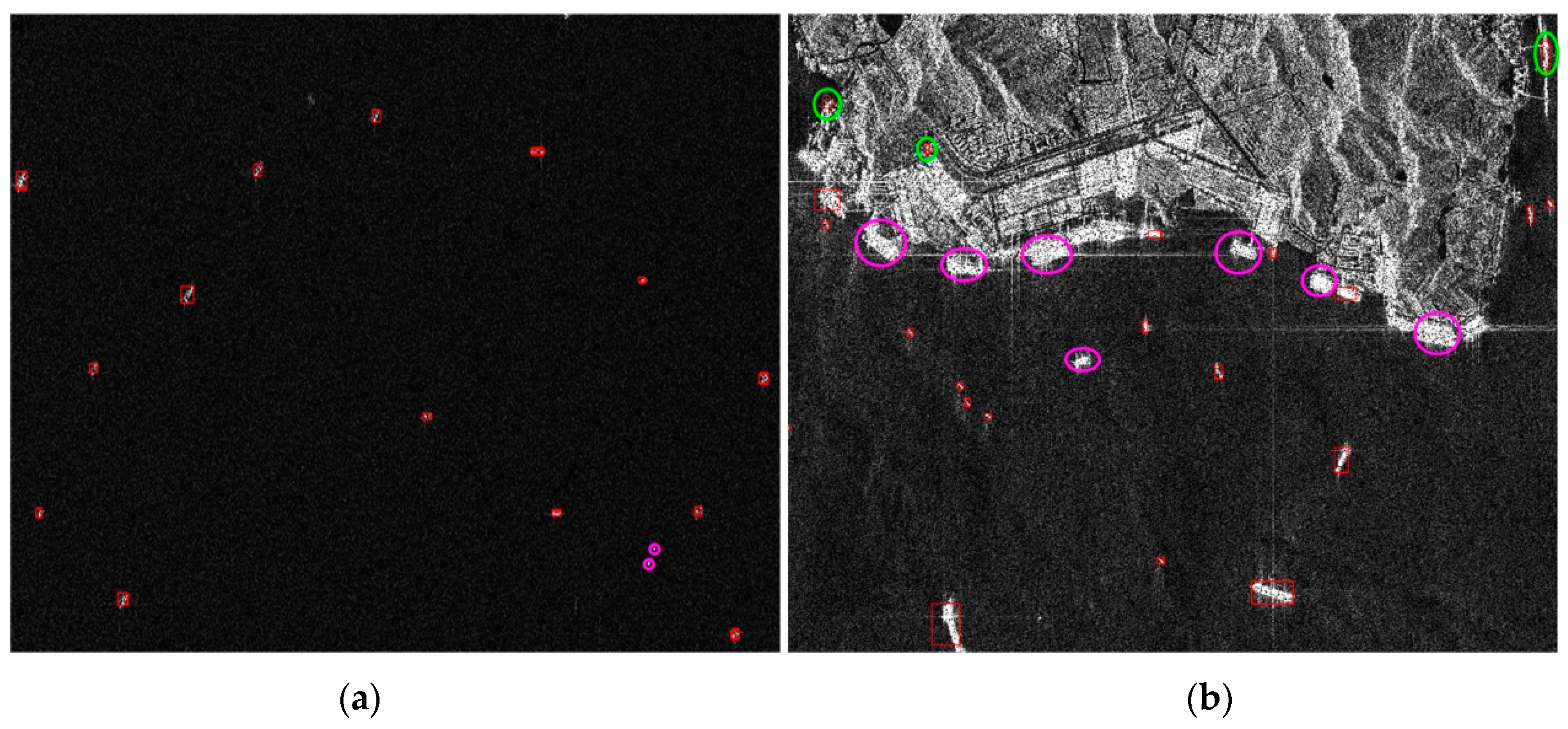
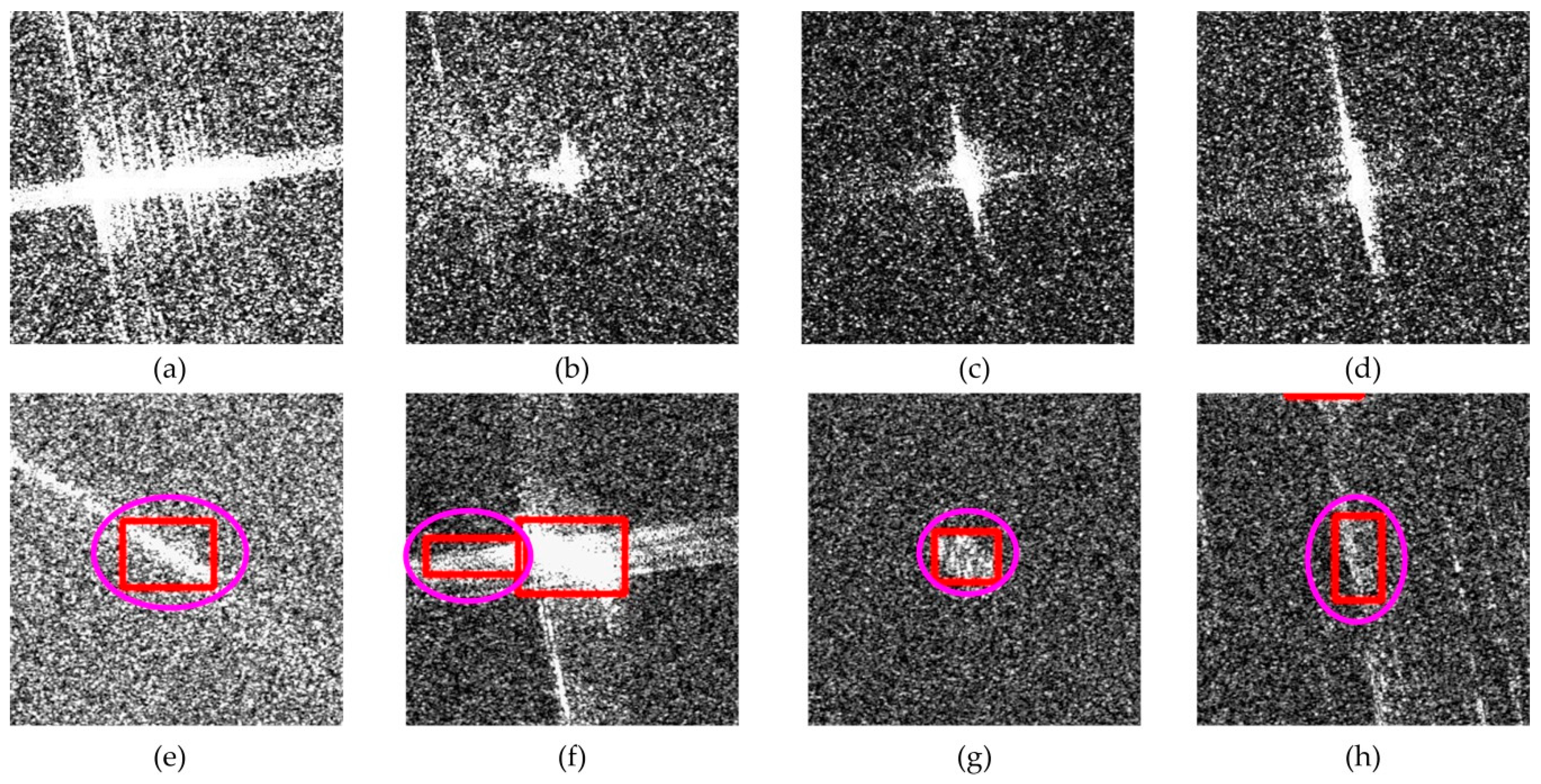
As shown earlier, RetinaNet achieves the best mAP (more than 96%) in multi-resolution SAR imagery. This high performance is due to the two core building blocks, i.e., FPN to extract the multi-scale semantic feature and focal loss to deal with the class imbalance and unfair contribution of hard/easy examples to the loss.
There are many factors that influence the performance of ship detection, such as image resolution, incidence angle, polarimetry, wind speed, sea state, ship size, and ship orientation. In Reference [4], an empirical model was employed to validate the ship size, incidence angle, wind speed, and sea state on the ship detectability. In this paper, we only explore the image resolution. The other factors have an impact on the scattering characteristics of the targets, thus affecting the detection results of ships. Next, we will continue to analyze the impact of other factors on ship detectability.
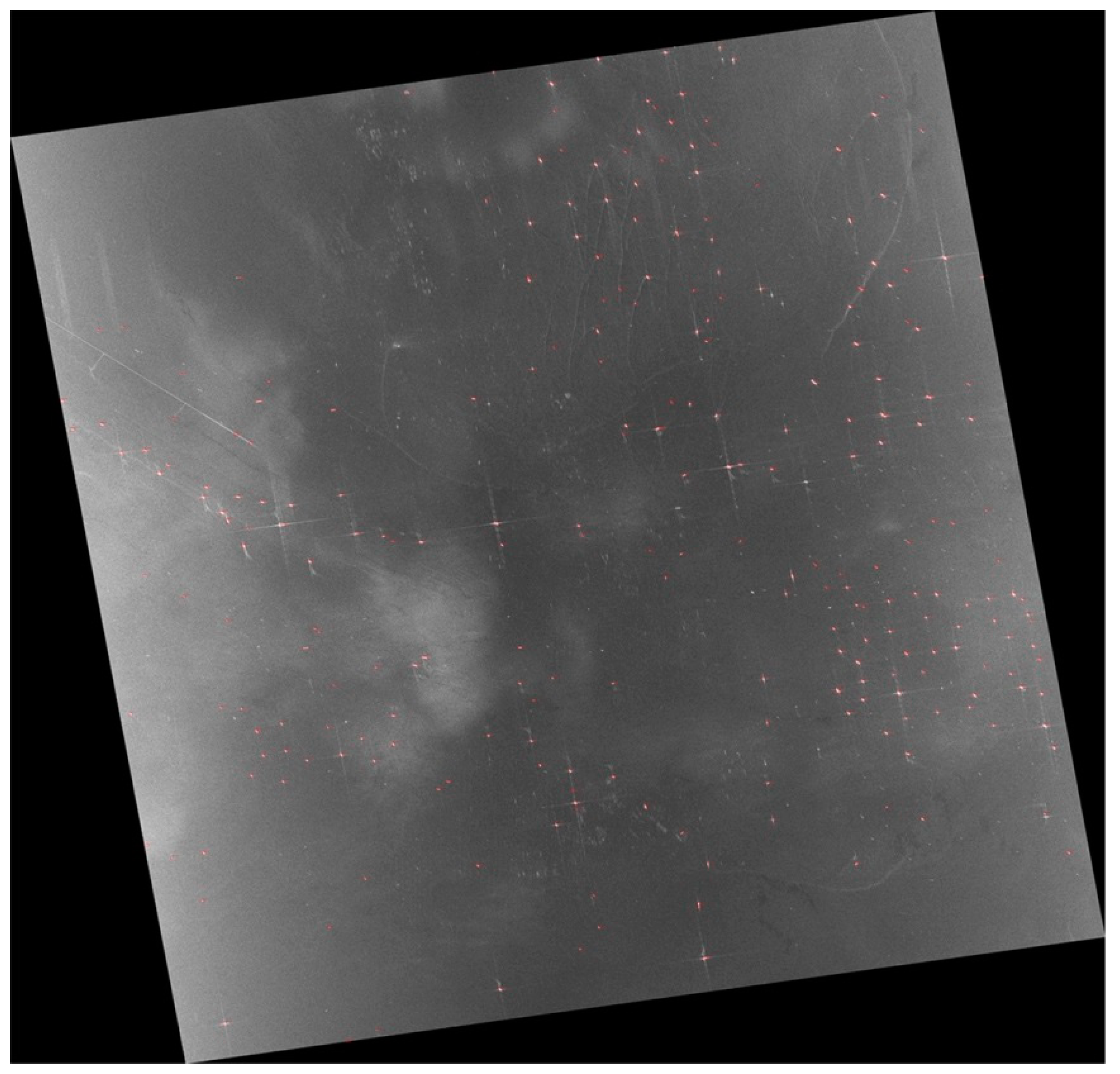
In addition, we find that preprocessing can also have a certain impact on the detection results. SAR images are converted to 8 bytes with a linear 2% stretch, which may cause a reduction in the ship detection performance. A better way to get chips is also being explored, and this dataset is planned to be released on our website [34]. One can also evaluate this based on our dataset.

5. Conclusions

In this paper, an object detector based on RetinaNet is applied to address ship detection in multi-resolution SAR imagery. First, a large volume of ship datasets cropped from multi-resolution SAR images is constructed. Second, RetinaNet with various settings, including FPN to extract the multi-scale semantic features and focal loss to crack the class imbalance and unequal contribution of hard and easy examples to the loss, is adapted to detect ships in SAR imagery. The experimental results reveal (1) even in multi-resolution SAR imagery, RetinaNet can achieve a high detection accuracy (up to 97% with regards to mAP) and (2) compared with other object detectors, RetinaNet achieves the best performance in complex backgrounds. Future work will focus on ship detection near the harbor.

Author Contributions

Y.W. was mainly responsible for the construction of the ship detection dataset, conceived the manuscript, and conducted the experiments. C.W. supervised the experiments and helped discuss the proposed method. H.Z. helped to acquire the Chinese Gaofen-3 SAR images and contributed to the organization of the paper, the revision of the paper, and the experimental analysis. S.W. and Y.D. participated in the construction of the dataset.

Funding

This research was funded by the National Key Research and Development Program of China (2016YFB0501501) and the National Natural Science Foundation of China under Grant 41331176.

Acknowledgments

We own many thanks to the China Center for Resources Satellite Data and Application for providing the Gaofen-3 images.

Conflicts of Interest

The authors declare no conflict of interest.

References

  1. Kang, M.; Ji, K.; Leng, X.; Lin, Z. Contextual region-based convolutional neural network with multilayer fusion for sar ship detection. Remote Sens. 2017, 9, 860. [Google Scholar] [CrossRef]
  2. Kang, M.; Leng, X.; Lin, Z.; Ji, K. A modified faster r-cnn based on cfar algorithm for sar ship detection. In Proceedings of the 2017 International Workshop on Remote Sensing with Intelligent Processing (RSIP), Shanghai, China, 18–21 May 2017; pp. 1–4. [Google Scholar]
  3. Wang, Y.; Wang, C.; Zhang, H. Combining a single shot multibox detector with transfer learning for ship detection using sentinel-1 sar images. Remote Sens. Lett. 2018, 9, 780–788. [Google Scholar] [CrossRef]
  4. Tings, B.; Bentes, C.; Velotto, D.; Voinov, S. Modelling ship detectability depending on terrasar-x-derived metocean parameters. CEAS Space J. 2018. [Google Scholar] [CrossRef]
  5. Smith, M.E.; Varshney, P.K. Vi-cfar: A novel cfar algorithm based on data variability. In Proceedings of the 1997 IEEE National Radar Conference, Syracuse, NY, USA, 13–15 May 1997; pp. 263–268. [Google Scholar]
  6. Gao, G.; Liu, L.; Zhao, L.; Shi, G.; Kuang, G. An adaptive and fast cfar algorithm based on automatic censoring for target detection in high-resolution sar images. IEEE Trans. Geosci. Remote Sens. 2009, 47, 1685–1697. [Google Scholar] [CrossRef]
  7. Farrouki, A.; Barkat, M. Automatic censoring cfar detector based on ordered data variability for nonhomogeneous environments. IEE Proc. Radar Sonar Navig. 2005, 152, 43–51. [Google Scholar] [CrossRef]
  8. El-Darymli, K.; Gill, E.W.; Mcguire, P.; Power, D.; Moloney, C. Automatic target recognition in synthetic aperture radar imagery: A state-of-the-art review. IEEE Access 2016, 4, 6014–6058. [Google Scholar] [CrossRef]
  9. Huang, X.; Yang, W.; Zhang, H.; Xia, G.-S. Automatic ship detection in sar images using multi-scale heterogeneities and an a contrario decision. Remote Sens. 2015, 7, 7695–7711. [Google Scholar] [CrossRef]
  10. Souyris, J.C.; Henry, C.; Adragna, F. On the use of complex sar image spectral analysis for target detection: Assessment of polarimetry. IEEE Trans. Geosci. Remote Sens. 2003, 41, 2725–2734. [Google Scholar] [CrossRef]
  11. Ouchi, K.; Tamaki, S.; Yaguchi, H.; Iehara, M. Ship detection based on coherence images derived from cross correlation of multilook sar images. IEEE Geosci. Remote Sens. Lett. 2004, 1, 184–187. [Google Scholar] [CrossRef]
  12. Kaplan, L.M. Improved sar target detection via extended fractal features. IEEE Trans. Aerosp. Electron. Syst. 2001, 37, 436–451. [Google Scholar] [CrossRef]
  13. Juanping, Z.; Weiwei, G.; Zenghui, Z.; Wenxian, Y. A coupled convolutional neural network for small and densely clustered ship detection in sar images. Sci. China Inf. Sci. 2019, 62, 042301. [Google Scholar] [CrossRef]
  14. El-Darymli, K.; McGuire, P.; Power, D.; Moloney, C.R. Target detection in synthetic aperture radar imagery: A state-of-the-art survey. J. Appl. Remote Sens. 2013, 7, 7–35. [Google Scholar]
  15. Goodfellow, I.; Bengio, Y.; Courville, A. Deep Learning; MIT Press: Cambridge, MA, USA, 2016. [Google Scholar]
  16. LeCun, Y.; Bengio, Y.; Hinton, G. Deep learning. Nature 2015, 521, 436–444. [Google Scholar] [CrossRef] [PubMed]
  17. Ren, S.; He, K.; Girshick, R.; Sun, J. Faster r-cnn: Towards real-time object detection with region proposal networks. IEEE Trans. Pattern Anal. Mach. Intell. 2017, 39, 1137–1149. [Google Scholar] [CrossRef] [PubMed]
  18. Liu, W.; Anguelov, D.; Erhan, D.; Szegedy, C.; Reed, S.E.; Fu, C.-Y.; Berg, A.C. Ssd: Single shot multibox detector. In Proceedings of the European Conference on Computer Vision (ECCV), Amsterdam, The Netherlands, 8–16 October 2016; pp. 21–37. [Google Scholar]
  19. Redmon, J.; Farhadi, A. Yolov3: An incremental improvement. arXiv, 2018; arXiv:1804.02767. [Google Scholar]
  20. Redmon, J.; Farhadi, A. Yolo9000: Better, faster, stronger. In Proceedings of the 2017 IEEE Conference on Computer Vision and Pattern Recognition (CVPR), Honolulu, HI, USA, 21–26 July 2017; pp. 6517–6525. [Google Scholar]
  21. Lin, T.; Goyal, P.; Girshick, R.; He, K.; Dollar, P. Focal loss for dense object detection. In Proceedings of the 2017 IEEE International Conference on Computer Vision (ICCV), Venice, Italy, 22–29 October 2017; pp. 2380–7504. [Google Scholar]
  22. Li, J.; Qu, C.; Shao, J. Ship detection in sar images based on an improved faster r-cnn. In Proceedings of the 2017 SAR in Big Data Era: Models, Methods and Applications (BIGSARDATA), Beijing, China, 13–14 November 2017; pp. 1–6. [Google Scholar]
  23. Lin, T.; Dollár, P.; Girshick, R.; He, K.; Hariharan, B.; Belongie, S. Feature pyramid networks for object detection. In Proceedings of the 2017 IEEE Conference on Computer Vision and Pattern Recognition (CVPR), Honolulu, HI, USA, 21–26 July 2017; pp. 936–944. [Google Scholar]
  24. Oliver, C.; Quegan, S. Understanding Synthetic Aperture Radar Images; SciTech Publ.: Shanghai, China, 2004. [Google Scholar]
  25. Liu, Y.; Zhang, M.H.; Xu, P.; Guo, Z.W. Sar ship detection using sea-land segmentation-based convolutional neural network. In Proceedings of the 2017 International Workshop on Remote Sensing with Intelligent Processing (RSIP), Shanghai, China, 18–21 May 2017; pp. 1–4. [Google Scholar]
  26. He, K.; Zhang, X.; Ren, S.; Sun, J. Deep residual learning for image recognition. In Proceedings of the 2016 IEEE Conference on Computer Vision and Pattern Recognition (CVPR), Las Vegas, NV, USA, 27–30 June 2016; pp. 770–778. [Google Scholar]
  27. Simonyan, K.; Zisserman, A. Very deep convolutional networks for large-scale image recognition. In Proceedings of the International Conference on Learning Representations (ICLR), San Diego, CA, USA, 7–9 May 2015. [Google Scholar]
  28. Huang, G.; Liu, Z.; Maaten, L.v.d.; Weinberger, K.Q. Densely connected convolutional networks. In Proceedings of the 2017 IEEE Conference on Computer Vision and Pattern Recognition (CVPR), Honolulu, HI, USA, 21–26 July 2017; pp. 2261–2269. [Google Scholar]
  29. Labelimg. Available online: https://github.com/tzutalin/labelImg (accessed on 6 May 2018).
  30. Keras: The Python Deep Learning Library. Available online: https://keras.io/ (accessed on 30 March 2018).
  31. Martín Abadi, P.B.; Chen, J.; Chen, Z.; Davis, A.; Dean, J.; Devin, M.; Ghemawat, S.; Irving, G.; Isard, M.; Kudlur, M.; et al. Tensorflow: A system for large-scale machine learning. In Proceedings of the 12th USENIX Conference on Operating Systems Design and Implementation (OSDI’16), Berkeley, CA, USA, 2–4 November 2016; pp. 265–283. [Google Scholar]
  32. Kingma, D.; Ba, J. Adam: A method for stochastic optimization. In Proceedings of the 2015 International Conference on Learning Representations (ICLR), San Diego, CA, USA, 7–9 May 2015. [Google Scholar]
  33. Schwegmann, C.P.; Kleynhans, W.; Salmon, B.P.; Mdakane, L.W.; Meyer, R.G.V. Very deep learning for ship discrimination in synthetic aperture radar imagery. In Proceedings of the 2016 IEEE International Geoscience and Remote Sensing Symposium (IGARSS), Beijing, China, 10–15 July 2016; pp. 104–107. [Google Scholar]
  34. SAR-Ship-Dataset. Available online: https://github.com/CAESAR-Radi/SAR-Ship-Dataset (accessed on 3 March 2019).
Figure 1. The architecture of RetinaNet: The green parts are the pyramidal features extracted by feature pyramid networks (FPN). The red and purple parts are the classification subnetworks and the box regression subnets, respectively. (a) indicates the backbone network and it can be VGG, ResNet, or DenseNet to extract features. (b) is FPN to obtain the multi-scale features. (c) illustrates that there are two subnets, i.e., the top red one for classification and the purple bottom for bounding box regression.
Remotesensing 11 00531 g001
Figure 2. The architecture of VGG16: The green boxes indicate the convolutional blocks, and the brown boxes represent the fully connected blocks. The four numbers that occur after each layer indicate the output number of the feature map, padding, kernel size, and stride, respectively.
Remotesensing 11 00531 g002
Figure 3. The architecture of FPN: C i   ( i = 1 , 2 , , 5 ) is used to denote the i th convolutional building g block as shown in Figure 2. The skipped connections apply a 1 × 1 convolution filter to reduce the depth of C i   ( i = 2 , 3 , 4 ) to 256. During the top-down flow, except the feature maps M 5 , M 2 , M 3 , and M 4 , first, the number of corresponding C i   ( i = 2 , 3 , 4 ) channels is reduced to 256 and then the layer is combined by upsampling the previous layer. Finally, a 3 × 3 convolution filter is used to obtain the feature map layers P i ( i = 2 , 3 , 4 , 5 ) for the classes and their locations.
Remotesensing 11 00531 g003
Figure 4. The experimental workflow of our proposed method: The black, blue, green, and red arrows represent the procedure of data process, model training, experimental test, and evaluation of robustness, respectively.
Remotesensing 11 00531 g004
Figure 5. The procedures for the construction of the labeled ship chips.
Remotesensing 11 00531 g005
Figure 6. Samples of the ship chips in the constructed dataset.
Remotesensing 11 00531 g006
Figure 7. The details of a labeled ship chip: The red, green, and cyan rectangles indicate the location of the ship, the object name, and the shape of the image in the left image, respectively.
Remotesensing 11 00531 g007
Figure 8. The area distribution of the bounding boxes includes the ships on the four resolution ((a) 3 m, (b) 5 m, (c) 8 m, and (d) 10 m) datasets and the whole dataset (e).
Remotesensing 11 00531 g008
Figure 9. The experimental robustness of the RetinaNet for ship detection in the (a) Ocean and (b) Harbor: The red rectangles, green ellipses, and magenta ellipses indicate the detected ships, false alarms, and the missing ships by the model.
Remotesensing 11 00531 g009
Figure 10. The ship detection results of the Cosmo-SkyMed imagery with the red rectangles indicating the location of ships.
Remotesensing 11 00531 g010
Figure 11. The four missing ships (ad) and four false alarms (eh): The ship chips (eh) are cropped from the whole image. The red rectangles and magenta ovals indicate the detected ships and false alarms, respectively.
Remotesensing 11 00531 g011
Table 1. The detailed information for several Chinese Gaofen-3 SAR images.
Imaging TimeResolution (m)Angle 1 (°) *Angle 2 (°) *Width *Height *Polarization *
21 October 2017836.7838.1764565959HH
5 April 2017835.337.0978946197HH
1 February 20181031.338.1728,42126,636HH
15 January 2017548.1150.2916,89827,760VH
13 November 2016541.4544.2316,33521,525HH
15 February 2017523.927.7320,86123,874HH
1 September 2017345.7147.1419,60920,998VV
1 September 2017334.8736.8116,78824,919HH
19 March 2018322.7525.0411,29120,350HH
14 March 2018333.6335.6216,33721,919HH
* Angle 1 is the near range incidence, and Angle 2 is the far range incidence. The width is the number of range pixels, and the height is the number of azimuth pixels.
Table 2. Six configurations of RetinaNet and their corresponding ship detection mean average precision (mAP).
ModelBackbone Network α t γ mAP (%)
RetinaNet-1VGG160.5296.77
RetinaNet-2VGG160.25197.2
RetinaNet-3VGG160.25297.56
RetinaNet-4VGG190.25296.48
RetinaNet-5Resnet500.25296.61
RetinaNet-6Resnet1520.25296.91
Table 3. The ship detection mAP of four models.
ModelSSDFaster RCNN FPNRetinaNet
mAP (%)72.5285.2691.5697.56
Table 4. The ship detection mAP for different resolutions.
Resolution3 m5 m8 m10 m
mAP_1 (%)96.3595.7897.2196.96
mAP_2 (%)97.9097.5897.9797.25
Table 5. The detailed information of the Cosmo-SkyMed image.
Imaging TimeResolutionAngle 1 (°) 1Angle 2 (°) 1Width 1Height 1Polarization
12 October 20173m43.1144.7318,29222,886VV
1 Angle 1 is the near range incidence, and Angle 2 is the far range incidence. The width is the number of range pixels, and the height is the number of azimuth pixels.
Table 6. The ship detection results validated with Automatic Identification System (AIS) for the Cosmo-SkyMed image.
Detected ShipsTrue ShipsFalse ShipsMissing ShipsDA (%)FA (%) F 1 Running Time (s)
29026822498.527.58%0.9538236.46
Table 7. The detailed AIS information on the 4 missing detected ships.
Ship IndexShip NameShip TypeMMSI 1Speed (knots)OrientationDestination
(a)XIN ZHOU9Cargo4134096901.8284.10SHANGHAI
(b)--4123555205.65101.00-
(c)BECKYCargo3534460007.36107.00CN CJK # 2
(d)--4133747802.782.00-
1 MMSI is short for Maritime Mobile Service Identity and is used to uniquely identify ships.

