A Remote Sensing Based Method to Detect Soil Erosion in Forests

 ,
, 
Abstract
1. Introduction
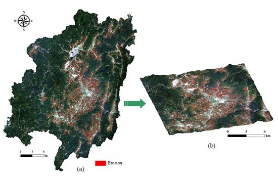
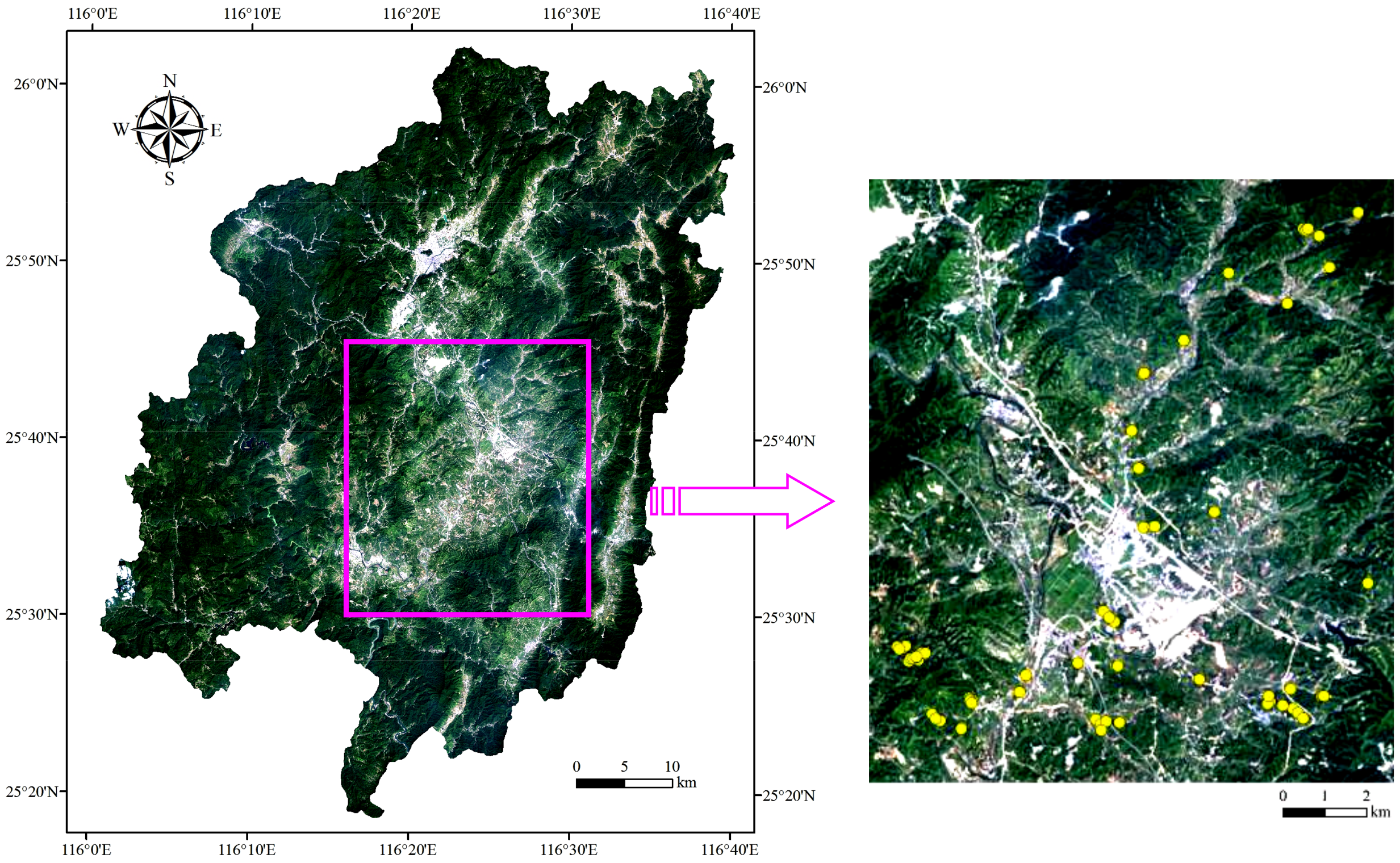
2. Study Area
3. Materials and Methods
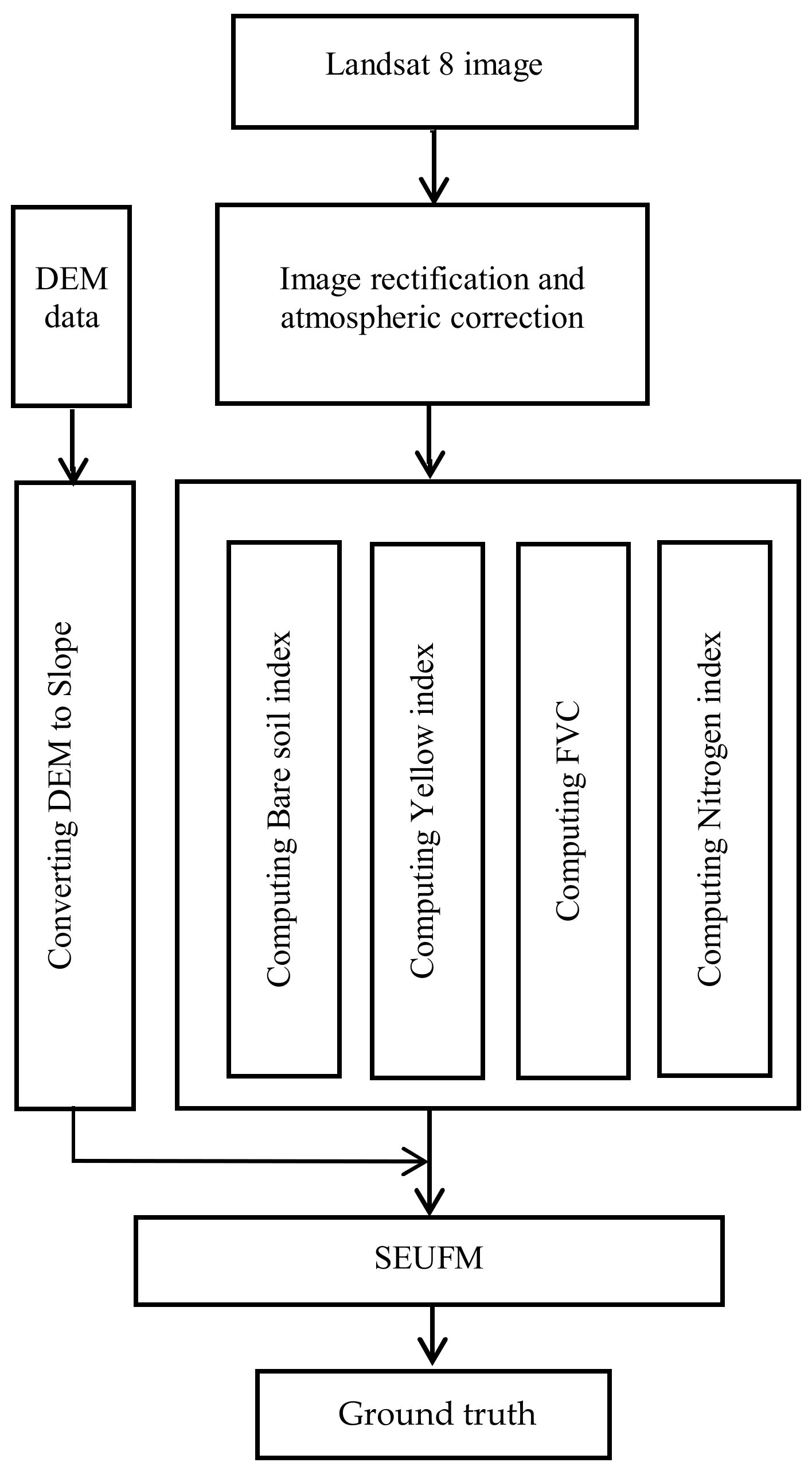
3.1. Remote Sensing Data and Image Pre-processing
3.2. Selection of Predictor Factors
3.3. Retrieval of the Selected Factors
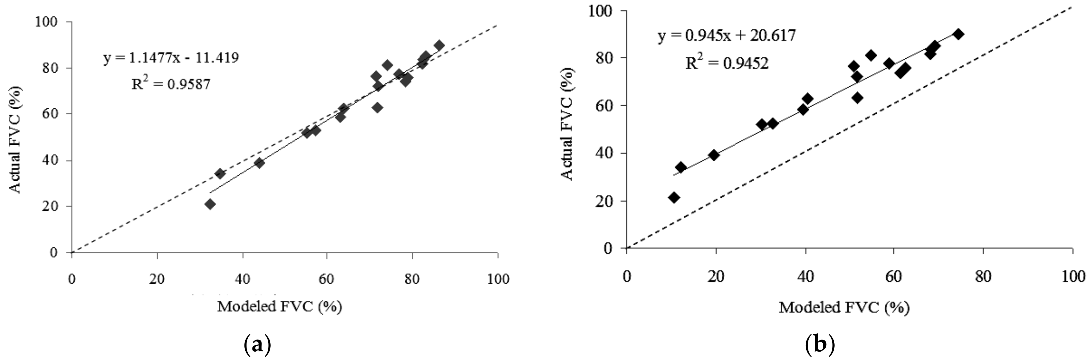
3.3.1. FVC
3.3.2. Nitrogen Reflectance Index (NRI)
3.3.3. Yellow Leaf Index (YLI)
3.3.4. Soil Exposure Index
3.3.5. Slope
3.4. Model Development
4. Results
4.1. Validation of Two FVC Models and Yellow Leaf Index (YLI)
4.2. Model Construction
4.2.1. PCA-based Model
4.4.2. Multiplication-based Model
4.3. Detecting Soil Erosion Potential in Forest
5. Discussion
6. Conclusions
Author Contributions
Funding
Acknowledgments
Conflicts of Interest
References
- Aiello, A.; Adamo, M.; Canora, F. Remote sensing and GIS to assess soil erosion with RUSLE3D and USPED at river basin scale in southern Italy. Catena 2015, 131, 174–185. [Google Scholar] [CrossRef]
- He, S.; Xie, J.; Yang, J. Status, causes and prevention of soil and water loss in Pinus massoniana woodland in hilly red soil region of southern China. Sci. Soil Water Conserv. 2011, 9, 65–70. [Google Scholar]
- Lei, H.Q. Soil and water loss of granite region under the trees in Xingguo County and its prevention and control. Soil Water Conserv China 2007, 3, 58–59. [Google Scholar]
- Zhu, S.Q.; Gong, J.; Lin, E.B. Discussion on characteristics of soil erosion under forest canopy in hilly area of southern China. Subtrop. Soil Water Conserv. 2013, 25, 24–30. [Google Scholar]
- Zhang, H.D.; Yu, D.S.; Dong, L.L.; Shi, X.Z.; Warner, E.; Gu, Z.J.; Sun, J.J. Regional soil erosion assessment from remote sensing data in rehabilitated high density canopy forests of southern China. Catena 2014, 123, 106–112. [Google Scholar] [CrossRef]
- Liao, C.; Wei, T. Characteristics of soil and water loss on red soil slope land under forest with different tree species. Bull. Soil Water Conserv. 2013, 33, 198–202. [Google Scholar]
- Xu, Y.B. Research on Process of Undergrowth Loss the Soil and Water in Red Soil Hilly Region of Southern China. Master’s Thesis, Fujian Normal University, Fuzhou, China, 2012. [Google Scholar]
- Renard, K.G.; Foster, G.R.; Weesies, G.A.; McCool, D.K.; Yoder, D.C. Predicting Soil Erosion by Water: A Guide to Conservation Planning with the Revised Universal Soil Loss Equation (RUSLE); U.S. Department of Agriculture: Washington, DC, USA, 1997.
- Wischmeier, W.H.; Smith, D.D. Predicting Rainfall Erosion Losses: A Guide to Conservation Planning; U.S. Department of Agriculture: Washington, DC, USA, 1978.
- Beasley, D.B.; Huggins, L.F.; Monke, E.J. Answers: A model for watershed planning. Trans. ASAE 1980, 23, 938–944. [Google Scholar] [CrossRef]
- Nearing, M.A.; Foster, G.R.; Lane, L.J.; Finkner, S.C. A process-based soil-erosion model for USDA-water erosion prediction project technology. Trans. ASAE 1989, 32, 1587–1593. [Google Scholar] [CrossRef]
- Engel, B.A.; Srinivasan, R.; Arnold, J.; Rewerts, C.; Brown, S.J. Nonpoint-source (NPS) pollution modeling using models integrated with geographic information systems (GIS). Water Sci. Technol. 1993, 28, 685–690. [Google Scholar] [CrossRef]
- Mitas, L.; Mitasova, H. Distributed erosion modeling for effective erosion prevention. Water Resour. Res. 1998, 34, 505–516. [Google Scholar] [CrossRef]
- Morgan, R.P.C.; Quinton, J.N.; Smith, R.E.; Govers, G.; Poesen, J.W.A.; Auerswald, K.; Chisci, G.; Torri, D.; Styczen, M.E. The European soil erosion model (EUROSEM): A dynamic approach for predicting sediment transport from fields and small catchments. Earth Surf. Process. Landf. 1998, 23, 527–544. [Google Scholar] [CrossRef]
- Roo, A.P.J.D.; Jetten, V.G. Calibrating and validating the LISEM model for two data sets from the Netherlands and South Africa. Catena 1999, 37, 477–493. [Google Scholar] [CrossRef]
- Jetten, V.G.; de Roo, A.P.J. Spatial analysis of erosion conservation measures with LISEM. In Landscape Erosion and Evolution Modeling; Harmon, R.S., Doe, W.W., Eds.; Springer: Boston, MA, USA, 2001; pp. 429–445. [Google Scholar]
- Coogle, A.L.; Lane, L.J.; Basher, L. Testing the Hillslope Erosion Model for Application in India, New Zealand and Australia. Environ. Model. Softw. 2003, 18, 825–830. [Google Scholar] [CrossRef]
- Merritt, W.S.; Letcher, R.A.; Jakeman, A.J. A review of erosion and sediment transport models. Environ. Model. Softw. 2003, 18, 761–799. [Google Scholar] [CrossRef]
- Chappell, A.; Zobeck, T.M.; Brunner, G. Using bi-directional soil spectral reflectance to model soil surface changes induced by rainfall and wind-tunnel abrasion. Remote Sens. Environ. 2006, 102, 328–343. [Google Scholar] [CrossRef]
- Mwaniki, M.W.; Agutu, N.O.; Mbaka, J.G.; Ngigi, T.G.; Waithaka, E.H. Landslide scar/soil erodibility mapping using Landsat TM/ETM+ bands 7 and 3 normalised difference index: A case study of central region of Kenya. Appl. Geogr. 2015, 64, 108–120. [Google Scholar] [CrossRef]
- Singh, D.; Herlin, I.; Berroir, J.P.; Silva, E.F.; Meirelles, M.S. An approach to correlate NDVI with soil colour for erosion process using NOAA/AVHRR data. Adv. Space Res. 2004, 33, 328–332. [Google Scholar] [CrossRef]
- Vrieling, A. Satellite remote sensing for water erosion assessment: A review. Catena 2006, 65, 2–18. [Google Scholar] [CrossRef]
- Xu, H.Q. Dynamic of soil exposure intensity and its effect on thermal environment change. Int. J. Climatol. 2014, 34, 902–910. [Google Scholar] [CrossRef]
- Sayao, V.M.; Dematte, J.A.M.; Bedin, L.G.; Nanni, M.R.; Rizzo, R. Satellite land surface temperature and reflectance related with soil attributes. Geoderma 2018, 325, 125–140. [Google Scholar] [CrossRef]
- Lobser, S.E.; Cohen, W.B. MODIS tasselled cap: land cover characteristics expressed through transformed MODIS data. Int. J. Remote Sens. 2007, 28, 5079–5101. [Google Scholar] [CrossRef]
- Metternicht, G.I.; Fermont, A. Estimating erosion surface features by linear mixture modeling. Remote Sens. Environ. 1998, 64, 254–265. [Google Scholar] [CrossRef]
- Guerschman, J.P.; Scarth, P.F.; McVicar, T.R.; Renzullo, L.J.; Malthus, T.J.; Stewart, J.B.; Rickards, J.E.; Trevithick, R. Assessing the effects of site heterogeneity and soil properties when unmixing photosynthetic vegetation, non-photosynthetic vegetation and bare soil fractions from Landsat and MODIS Data. Remote Sens. Environ. 2015, 161, 12–26. [Google Scholar] [CrossRef]
- Shruthi, R.; Kerle, N.; Jetten, V.; Abdellah, L.; Machmach, I. Quantifying temporal changes in gully erosion areas with object oriented analysis. Catena 2015, 128, 262–277. [Google Scholar] [CrossRef]
- Rahmati, O.; Tahmasebipour, N.; Haghizadeh, A.; Pourghasemi, H.R.; Feizizadeh, B. Evaluating the influence of geo-environmental factors on gully erosion in a semi-arid region of Iran: An integrated framework. Sci. Total Environ. 2017, 579, 913–927. [Google Scholar] [CrossRef] [PubMed]
- Garosi, Y.; Sheklabadi, M.; Pourghasemi, H.R.; Besalatpour, A.A.; Conoscenti, C.; Van Oost, K. Comparison of differences in resolution and sources of controlling factors for gully erosion susceptibility mapping. Geoderma 2018, 330, 65–78. [Google Scholar] [CrossRef]
- Cheng, Z.L.; Lu, D.S.; Li, G.Y.; Huang, J.Q.; Sinha, N.; Zhi, J.J.; Li, S.J. A random forest-based approach to map soil erosion risk distribution in Hickory Plantations in western Zhejiang Province, China. Remote Sens. 2018, 10, 1899. [Google Scholar] [CrossRef]
- Leek, R.; Solberg, R. Using remote-sensing for monitoring of autumn tillage in Norway. Int. J. Remote Sens. 1995, 16, 447–466. [Google Scholar] [CrossRef]
- Khawlie, M.; Awad, M.; Shaban, A.; Kheir, R.B.; Abdallah, C. Remote sensing for environmental protection of the eastern Mediterranean rugged mountainous areas, Lebanon. ISPRS J. Photogramm. 2002, 57, 13–23. [Google Scholar] [CrossRef]
- d’Oleire-Oltmanns, S.; Marzolff, I.; Peter, K.D.; Ries, J.B. Unmanned Aerial Vehicle (UAV) for monitoring soil erosion in Morocco. Remote Sens. 2012, 4, 3390–3416. [Google Scholar] [CrossRef]
- Chen, J.J.; Yi, S.H.; Qin, Y.; Wang, X.Y. Improving estimates of fractional vegetation cover based on UAV in alpine grassland on the Qinghai-Tibetan Plateau. Int. J. Remote Sens. 2016, 37, 1922–1936. [Google Scholar] [CrossRef]
- Neugirg, F.; Stark, M.; Kaiser, A.; Vlacilova, M.; Seta, M.D.; Vergari, F.; Schmidt, J.; Becht, M.; Haas, F. Erosion processes in calanchi in the Upper Orcia Valley, Southern Tuscany, Italy based on multitemporal high-resolution terrestrial LiDAR and UAV surveys. Geomorphology 2016, 269, 8–22. [Google Scholar] [CrossRef]
- Verstraeten, G.; Poesen, J.; Demaree, G.; Salles, C. Long-term (105 years) variability in rain erosivity as derived from 10-min rainfall depth data for Ukkel (Brussels, Belgium): Implications for assessing soil erosion rates. J. Geophys. Res. Atmos. 2006, 111, D22109. [Google Scholar] [CrossRef]
- Piacentini, T.; Galli, A.; Marsala, V.; Miccadei, E. Analysis of Soil Erosion Induced by Heavy Rainfall: A Case Study from the NE Abruzzo Hills Area in Central Italy. Water 2018, 10, 1314. [Google Scholar] [CrossRef]
- Li, X.; Zhang, X.; Zhang, L.; Wu, B. Rainfall and Vegetation Coupling Index for soil erosion risk mapping. J. Soil Water Conserv. 2014, 69, 213–220. [Google Scholar] [CrossRef]
- Yin, S.; Zhu, Z.Y.; Wang, L.; Liu, B.Y.; Xie, Y.; Wang, G.N.; Li, Y.S. Regional soil erosion assessment based on a sample survey and geostatistics. Hydrol. Earth Syst. Sci. 2018, 22, 1695–1712. [Google Scholar] [CrossRef]
- Mateos, E.; Miguel, E.J.; Ormaetxea, L. Soil erosion and forests biomass as energy resource in the basin of the Oka River in Biscay, northern Spain. Forests 2017, 8, 258. [Google Scholar] [CrossRef]
- Ochoa, P.A.; Fries, A.; Mejia, D.; Burneo, J.I.; Ruiz-Sinoga, J.D.; Cerda, A. Effects of climate, land cover and topography on soil erosion risk in a semiarid basin of the Andes. Catena 2016, 140, 31–42. [Google Scholar] [CrossRef]
- Meusburger, K.; Baenninger, D.; Alewell, C. Estimating vegetation parameter for soil erosion assessment in an alpine catchment by means of QuickBird imagery. Int. J. Appl. Earth Obs. 2010, 12, 201–207. [Google Scholar] [CrossRef]
- Molina, A.; Govers, G.; Poesen, J.; Van Hemelryck, H.; De Bievre, B.; Vanacker, V. Environmental factors controlling spatial variation in sediment yield in a central Andean mountain area. Geomorphology 2008, 98, 176–186. [Google Scholar] [CrossRef]
- Panagos, P.; Borrelli, P.; Meusburger, K.; Alewell, C.; Lugato, E.; Montanarella, L. Estimating the soil erosion cover-management factor at the European scale. Land Use Policy 2015, 48, 38–50. [Google Scholar] [CrossRef]
- Schonbrodt, S.; Saumer, P.; Behrens, T.; Seeber, C.; Scholten, T. Assessing the USLE crop and management factor C for soil erosion modeling in a large mountainous watershed in Central China. J. Earth Sci. 2010, 21, 835–845. [Google Scholar] [CrossRef]
- Yang, X.H. Deriving RUSLE cover factor from time-series fractional vegetation cover for hillslope erosion modelling in New South Wales. Soil Res. 2014, 52, 253–261. [Google Scholar] [CrossRef]
- Foerster, S.; Wilczok, C.; Brosinsky, A.; Segl, K. Assessment of sediment connectivity from vegetation cover and topography using remotely sensed data in a dryland catchment in the Spanish Pyrenees. J. Soils Sediment. 2014, 14, 1982–2000. [Google Scholar] [CrossRef]
- Kinnell, P.I.A.; Wang, J.; Zheng, F. Comparison of the abilities of WEPP and the USLE-M to predict event soil loss on steep loessal slopes in China. Catena 2018, 171, 99–106. [Google Scholar] [CrossRef]
- Qin, C.Z.; Gao, H.R.; Zhu, L.J.; Zhu, A.X.; Liu, J.Z.; Wu, H. Spatial optimization of watershed best management practices based on slope position units. J. Soil Water Conserv. 2018, 73, 504–517. [Google Scholar] [CrossRef]
- Dai, Q.; Peng, X.; Wang, P.J.; Li, C.; Shao, H.B. Surface erosion and underground leakage of yellow soil on slopes in karst regions of southwest China. Land Degrad. Dev. 2018, 29, 2438–2448. [Google Scholar] [CrossRef]
- Chavez, P.S. Image-based atmospheric corrections revisited and improved. Photogramm. Eng. Remote Sens. 1996, 62, 1025–1036. [Google Scholar]
- Xu, H.Q. Retrieval of the reflectance and land surface temperature of the newly-launched Landsat 8 satellite. Chin. J. Geophys. China 2015, 58, 741–747. [Google Scholar]
- Hu, X.J.; Xu, H.Q.; Guo, Y.B.; Zhang, B.B. Remote sensing detection of vegetation health status after ecological restoration in soil and water loss region. Chin. J. Appl. Ecol. 2017, 38, 250–256. [Google Scholar]
- Schmitter, P.; Kibret, K.S.; Lefore, N.; Barron, J. Suitability mapping framework for solar photovoltaic pumps for smallholder farmers in Sub-Saharan Africa. Appl. Geogr. 2018, 94, 41–57. [Google Scholar] [CrossRef]
- Xu, H.Q.; He, H.; Huang, S.L. Analysis of fractional vegetation cover change and its impact on thermal environment in the Hetian basinal area of County Changting, Fujian Province, China. Acta Ecol. Sin. 2013, 33, 2954–2963. [Google Scholar]
- Ministry of Water Resources of China. Standards for Classification and Gradation of Soil Erosion; SL 190-2007; Ministry of Water Resources of China: Beijing, China, 2008.
- Blanco, H.; Lal, R. Principles of Soil Conservation and Management; Springer: Heidelberg, Germany, 2010. [Google Scholar]
- Yan, C.Y.; Liu, Q.; Niu, Z.; Wang, C.Y. Inversion of vegetation biochemicals by remote sensing. J. Remote Sens. 2004, 8, 300–308. [Google Scholar]
- Zhou, G.Y.; Morris, J.D.; Yan, J.H.; Yu, Z.Y.; Peng, S.L. Hydrological impacts of reafforestation with eucalypts and indigenous species: A case study in southern China. For. Ecol. Manag. 2002, 167, 209–222. [Google Scholar] [CrossRef]
- Sun, J. Using LAI Express the Effect of Vegetation in Preventing Soil Erosion and Vegetation Recovering Degree. Ph.D. Thesis, Institute of Soil Science, Chinese Academy of Sciences, Beijing, China, 2010. [Google Scholar]
- Franceschini, M.H.D.; Dematte, J.A.M.; Terra, F.D.; Vicente, L.E.; Bartholomeus, H.; de Souza, C.R. Prediction of soil properties using imaging spectroscopy: Considering fractional vegetation cover to improve accuracy. Int. J. Appl. Earth Obs. 2015, 38, 358–370. [Google Scholar] [CrossRef]
- Carlson, T.N.; Ripley, D.A. On the relation between NDVI, fractional vegetation cover, and leaf area index. Remote Sens. Environ. 1997, 62, 241–252. [Google Scholar] [CrossRef]
- Gutman, G.; Ignatov, A. The derivation of the green vegetation fraction from NOAA/AVHRR data for use in numerical weather prediction models. Int. J. Remote Sens. 1998, 19, 1533–1543. [Google Scholar] [CrossRef]
- Zhou, X.; Guan, H.D.; Xie, H.; Wilson, J.L. Analysis and optimization of NDVI definitions and areal fraction models in remote sensing of vegetation. Int. J. Remote Sens. 2009, 30, 721–751. [Google Scholar] [CrossRef]
- Wu, C.S.; Murray, A.T. Estimating impervious surface distribution by spectral mixture analysis. Remote Sens. Environ. 2003, 84, 493–505. [Google Scholar] [CrossRef]
- Bausch, W.C.; Duke, H.R. Remote sensing of plant nitrogen status in corn. Trans. ASAE 1996, 39, 1869–1875. [Google Scholar] [CrossRef]
- Jensen, J.R. Remote Sensing of the Environment: An Earth Resource Perspective, 2nd ed.; Pearson Prentice-Hall Inc.: Upper Saddle River, NJ, USA, 2006. [Google Scholar]
- Jensen, J.R. Introductory Digital Image Processing: A Remote Sensing Perspective, 4th ed.; Pearson Prentice-Hall Inc.: Upper Saddle River, NJ, USA, 2015. [Google Scholar]
- Hill, J.; Schutt, B. Mapping complex patterns of erosion and stability in dry Mediterranean ecosystems. Remote Sens. Environ. 2000, 74, 557–569. [Google Scholar] [CrossRef]
- Kearney, M.S.; Rogers, A.S.; Townshend, J.R.G. Developing a model for determining coastal marsh “health”. In Proceedings of the Third Thematic Conference on Remote Sensing for Marine and Coastal Environments, Seattle, WA, USA, 18–20 September 1995; pp. 527–537. [Google Scholar]


| WorldView 2 | WorldView 2 Yellow Band (Invariant Patches) | Landsat 8 Simulated Yellow Band (Invariant Patches) | ||
|---|---|---|---|---|
| Yellow Band | Simulated Yellow Band | |||
| Mean | 0.055 | 0.054 | 0.055 | 0.063 |
| Std Dev | 0.034 | 0.032 | 0.032 | 0.030 |
| R2 | 0.984 | 0.928 | ||
| PC1 | PC2 | PC3 | PC4 | PC5 | |
|---|---|---|---|---|---|
| FVC | −0.621 | −0.219 | −0.049 | 0.223 | 0.717 |
| NRI | −0.466 | −0.129 | 0.778 | −0.256 | −0.310 |
| NDSI | 0.361 | 0.181 | 0.553 | 0.705 | 0.187 |
| YLI | 0.404 | 0.105 | 0.293 | −0.621 | 0.595 |
| Slope | −0.322 | 0.944 | −0.043 | −0.050 | 0.022 |
| Eigenvalue | 0.129 | 0.021 | 0.006 | 0.004 | 0.001 |
| Percent eigenvalue (%) | 80.12 | 13.04 | 3.73 | 2.48 | 0.62 |
| Soil Erosion | Non-Soil Erosion | Percent Difference (%) | p-Value | |||||||
|---|---|---|---|---|---|---|---|---|---|---|
| Min | Max | Mean | Std Dev | Min | Max | Mean | Std Dev | |||
| Slope | 0.070 | 0.541 | 0.219 | 0.096 | 0.026 | 0.397 | 0.206 | 0.135 | 6.31 | 0.821 |
| FVC | 0.454 | 0.785 | 0.651 | 0.074 | 0.721 | 0.897 | 0.804 | 0.064 | −19.03 | 0.000 |
| NRI | 0.283 | 0.467 | 0.358 | 0.040 | 0.375 | 0.594 | 0.476 | 0.065 | −24.78 | 0.003 |
| NDSI | 0.069 | 0.524 | 0.283 | 0.084 | 0.110 | 0.275 | 0.184 | 0.049 | 53.80 | 0.001 |
| YLI | 0.214 | 0.433 | 0.309 | 0.049 | 0.172 | 0.292 | 0.226 | 0.048 | 36.73 | 0.004 |
| Mean/Initial Threshold | Final Threshold | Threshold to Mean | |
|---|---|---|---|
| SEUFM1 | 0.355 | 0.371 | 1.045 |
| SEUFM1+2 | 0.350 | 0.366 | 1.046 |
| SEUFMm-slope | 0.153 | 0.166 | 1.089 |
| SEUFMm+slope | 0.088 | 0.079 | 0.898 |
| Erosion | Non-Erosion | Total | User’s Accuracy % | |
|---|---|---|---|---|
| SEUFM1 (threshold: 0.371) | ||||
| Erosion | 51 | 2 | 53 | 96.23 |
| Non-Erosion | 6 | 20 | 26 | 76.92 |
| Total | 57 | 22 | 79 | |
| Producer’s accuracy (%) | 89.47 | 90.91 | ||
| Overall accuracy (%) | 89.87 | Kappa | 0.761 | |
| SEUFM1+2 (threshold: 0.366) | ||||
| Erosion | 44 | 6 | 50 | 88.00 |
| Non- Erosion | 13 | 16 | 29 | 55.17 |
| Total | 57 | 22 | 79 | |
| Producer’s accuracy (%) | 77.19 | 72.73 | ||
| Overall accuracy (%) | 75.95 | Kappa | 0.455 | |
| SEUFMm-slope (threshold: 0.166) | ||||
| Erosion | 48 | 6 | 54 | 88.89 |
| Non-Erosion | 9 | 16 | 25 | 64.00 |
| Total | 57 | 22 | 79 | |
| Producer’s accuracy (%) | 84.21 | 72.73 | ||
| Overall accuracy (%) | 81.01 | Kappa | 0.547 | |
| SEUFMm+slope (threshold: 0.079) | ||||
| Erosion | 40 | 10 | 50 | 80.00 |
| Non-Erosion | 17 | 12 | 29 | 41.38 |
| Total | 57 | 22 | 79 | |
| Producer’s accuracy (%) | 70.18 | 54.55 | ||
| Overall accuracy (%) | 65. 82 | Kappa | 0.225 | |
| Slope | FVC | NRI | NDSI | YLI | |
|---|---|---|---|---|---|
| Slope | 1.000 | ||||
| FVC | 0.414 | 1.000 | |||
| NRI | 0.406 | 0.869 | 1.000 | ||
| NDSI | −0.324 | −0.829 | −0.705 | 1.000 | 0.767 |
| YLI | −0.421 | −0.897 | −0.759 | 0.767 | 1.000 |
© 2019 by the authors. Licensee MDPI, Basel, Switzerland. This article is an open access article distributed under the terms and conditions of the Creative Commons Attribution (CC BY) license (http://creativecommons.org/licenses/by/4.0/).
Share and Cite
Xu, H.; Hu, X.; Guan, H.; Zhang, B.; Wang, M.; Chen, S.; Chen, M. A Remote Sensing Based Method to Detect Soil Erosion in Forests. Remote Sens. 2019, 11, 513. https://doi.org/10.3390/rs11050513
Xu H, Hu X, Guan H, Zhang B, Wang M, Chen S, Chen M. A Remote Sensing Based Method to Detect Soil Erosion in Forests. Remote Sensing. 2019; 11(5):513. https://doi.org/10.3390/rs11050513
Chicago/Turabian StyleXu, Hanqiu, Xiujuan Hu, Huade Guan, Bobo Zhang, Meiya Wang, Shanmu Chen, and Minghua Chen. 2019. "A Remote Sensing Based Method to Detect Soil Erosion in Forests" Remote Sensing 11, no. 5: 513. https://doi.org/10.3390/rs11050513
APA StyleXu, H., Hu, X., Guan, H., Zhang, B., Wang, M., Chen, S., & Chen, M. (2019). A Remote Sensing Based Method to Detect Soil Erosion in Forests. Remote Sensing, 11(5), 513. https://doi.org/10.3390/rs11050513