Abstract
Geographic object-based image analysis (GEOBIA) has been widely used in the remote sensing of agricultural crops. However, issues related to image segmentation, data redundancy and performance of different classification algorithms with GEOBIA have not been properly addressed in previous studies, thereby compromising the accuracy of subsequent thematic products. It is in this regard that the current study investigates the optimal scale parameter (SP) in multi-resolution segmentation, feature subset, and classification algorithm for use in GEOBIA based on multisource satellite imagery. For this purpose, a novel supervised optimal SP selection method was proposed based on information gain ratio, and was then compared with a preexisting unsupervised optimal SP selection method. Additionally, the recursive feature elimination (RFE) and enhanced RFE (EnRFE) algorithms were modified to generate an improved EnRFE (iEnRFE) algorithm, which was then compared with its precursors in the selection of optimal classification features. Based on the above, random forest (RF), gradient boosting decision tree (GBDT) and support vector machine (SVM) were applied to segmented objects for crop classification. The results indicated that the supervised optimal SP selection method is more suitable for application in heterogeneous land cover, whereas the unsupervised method proved more efficient as it does not require reference segmentation objects. The proposed iEnRFE method outperformed the preexisting EnRFE and RFE methods in optimal feature subset selection as it recorded the highest accuracy and less processing time. The RF, GBDT, and SVM algorithms achieved overall classification accuracies of 91.8%, 92.4%, and 90.5%, respectively. GBDT and RF recorded higher classification accuracies and utilized much less computational time than SVM and are, therefore, considered more suitable for crop classification requiring large numbers of image features. These results have shown that the proposed object-based crop classification scheme could provide a valuable reference for relevant applications of GEOBIA in crop recognition using multisource satellite imagery.
1. Introduction
The acquisition of reliable crop distribution maps is becoming increasingly important for agricultural land management amidst growing food demands in response to an ever-increasing human population globally [1]. In recent years, with the continuous launch of satellites such as Landsat-8 and Sentinel-2, crop classification based on multisource medium-high resolution images has become an efficient alternative that resolves the inadequacies of insufficient time resolution of a single optical satellite, especially in cloud-prone areas (tropics and subtropics) [2,3,4].
Geographic object-based image analysis (GEOBIA) is an important approach to the use of multisource satellite imagery in crop classification [5,6]. It takes geographic objects rather than pixels as the basic unit of classification, which avoids the salt and pepper phenomenon typical of traditional pixel-based classifiers like maximum likelihood, and could deal with the problem of inconsistent spatial resolution among multisource data [7,8,9]. Moreover, with the addition of texture and shape information, object-based classification can employ more features in recognizing target objects [10,11,12,13]. However, despite its advantages over traditional classifiers, the use of GEOBIA is also constrained by uncertainties associated with image segmentation [14], feature selection [15,16] and classification algorithms [17,18]. Segmentation is an essential process in GEOBIA, and the definition of segmentation parameters could have a significant influence on classification accuracy [19,20,21]. While the introduction of abundant features brings additional information that is relevant in target recognition, it could also introduce noise or redundant information that can degrade classification accuracy [22,23]. Moreover, several classification algorithms have been proposed and their performances (accuracy, efficiency and feasibility) in GEOBIA vary considerably [24,25,26]. Therefore, in order to exploit the full potential of GEOBIA in crop recognition with multisource satellite imagery, the optimal combination of segmentation, feature selection and classification algorithms needs to be identified, hence the current study.
Multi-resolution segmentation is the most widely used segmentation method in GEOBIA, and it takes a bottom-up segmentation approach based on a pair-wise region merging technique [5,21]. A key parameter in multi-resolution segmentation is scale. An excessively large scale will result in under-segmentation, while an excessively small scale will result in over-segmentation [27,28]. The traditional method to determine the optimal scale parameter (SP) of multi-resolution segmentation is trial and error, which is not only subjective but also time-consuming [29]. In an effort to quantitatively determine optimal SP and improve automation, some supervised and unsupervised algorithms have been developed [30,31,32,33,34]. Supervised methods use ‘real’ objects to assess the reliability of segmentation results, while unsupervised methods use varieties of heterogeneity and homogeneity measures to assess the segmentation results [35]. Although the unsupervised method is less time-consuming when compared with the supervised method, the latter has been found to be more accurate. Based on a critical review of relevant articles published in three major remote-sensing journals in the recent past, Costa et al. [36] concluded that image segmentation accuracy assessment is still in its infancy and little attention has been paid to assessing the relative competencies of supervised and unsupervised methods. Moreover, performing a supervised optimal SP selection is still challenging owing to the complexity of measuring the differences between segmented and ‘real’ objects, in addition to being difficult and time-consuming in acquiring reference objects over large areas [37]. Studies that assess the potential of acquiring reference objects from representative areas for application at large scales are, therefore, required to minimize time while not compromising accuracy.
Object-based classification could generate dozens or hundreds of features. An excessive number of features may cause difficulties in training classification models and could result in a poor classification performance, known as the Hughes phenomenon [38]. Thus, assessing the importance of features and selecting optimal feature subsets could be helpful for improving the classification accuracy [39]. A series of measures such as variance [40], chi-square [41], Relief-F [42] and correlation [43] have been used to obtain the optimal feature subset, while machine learning algorithms like random forest (RF) can also provide variable importance that is useful in feature selection [44,45]. However, a feature of low importance may have a great impact on classification accuracy when combined with other features [46]. By this consideration, assessing the performance of a feature subset directly through its classification accuracy would be more appropriate. It is also important to note that when the number of features is large, it is difficult to evaluate the accuracy of all possible feature combinations due to the huge computational work and time required. Thus for operational purposes, a series of search strategies are used in screening the most optimal feature subset [22,47]. However, few studies have evaluated the performance of these feature selection methods especially in GEOBIA crop recognition applications involving multisource satellite imagery.
Several classification algorithms are available for application on segmented objects and optimal features for crop recognition with GEOBIA. With the rapid development of machine learning in recent years, image classification algorithms and tools have increasingly been provided, and their application in crop recognition has become universal. Commonly-used machine learning methods include C4.5 [48], classification and regression tree (CART) [49], RF [44], support vector machine (SVM) [45] and gradient boosting decision tree (GBDT) [50]. Several differences exist among these machine-learning methods, including parameter settings, accuracy performance and efficiency. Therefore, it is necessary to evaluate these machine-learning methods so as to arrive at the most suitable for operational crop recognition initiatives involving GEOBIA and multisource satellite imagery.
Previous studies have evaluated the effect of one or two of the three factors (segmentation, feature selection and classification algorithm) on GEOBIA in land-cover mapping. Duro et al. [51] compared three machine-learning algorithms including RF, SVM and decision tree (DT) for an object-based image analysis that utilizes the ‘trial-and-error’ approach to determining optimal SP while relying on expert knowledge in selecting optimal object features. Liu et al. [52] compared the performances of fully convolutional networks (FCN), RF and SVM in GEOBIA based on a fixed segmentation scale parameter and involving all features. Based on a fixed segmentation scale parameter, Ma et al. [53] compared the results obtained from three feature-subset evaluation methods in GEOBIA using SVM and RF. To the best of our knowledge, no study has reported to date the combined effect of the aforementioned three factors in GEOBIA.
In view of the research gaps in the use of GEOBIA in crop recognition outlined in the above paragraphs, this paper, based on the information gain ratio, proposed a novel supervised optimal SP selection method for comparison with an unsupervised optimal SP selection method. Additionally, based on the recursive feature elimination (RFE) [54] and enhanced RFE (EnRFE) [22] algorithms, this paper proposed an improved EnRFE (iEnRFE) algorithm for the selection of the optimal feature subset for GEOBIA. Using the optimal segmentation scale parameter and feature subset, the widely used classification algorithms of RF, SVM and GBDT were evaluated for accuracy and efficiency in crop recognition with GEOBIA and multisource satellite imagery (Sentinel-2A, Landsat-8 OLI and GF-1 WFV), and results obtained are envisaged to provide a valuable reference for relevant operational scenarios.
2. Materials
2.1. Study Area
Located in the Jiangsu Province of East China, Xinghua County is used as test site (Figure 1). It has a total area of 2353 km² and a population size of about 1.5 million. Xinghua County is within the subtropical monsoon climate zone, with an average annual temperature range of 14 °C to 15 °C and an annual precipitation total of approximately 1040.4 mm. The relatively flat topography and warm-moist climate of this area favors aquaculture and agriculture, making it one of the major food producing areas of China.
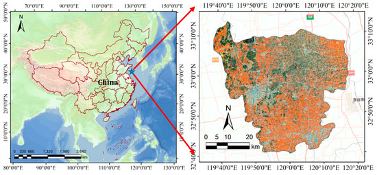
Figure 1.
Location of Xinghua County in Jiangsu Province.
The main summer crop is paddy rice [55], whereas winter wheat (Triticum aestivum L.) and oilseed rape (Brassica napus L.) [56] dominate the winter season. Green Onion (Allium ascalonicum) is planted year-round and can be harvested 3 to 4 times a year [57].
2.2. Image Acquisition and Preprocessing
In order to obtain enough clear sky images that cover the main phenological stages of the crops under investigation in Xinghua, only satellite images whose footprint over Xinhua is 100% cloud-free were downloaded for the current study. In this regard, only five images from the multisource fulfilled this criterion and they included two images of the Sentinel-2A Multispectral Instrument (MSI), two images of the Landsat-8 Operational Land Imager (OLI) and one image obtained from GF-1 Wide Field of View (WFV). Sentinel-2A images were acquired on 28 February and 29 April 2017, Landsat images were acquired on 15 March and 18 May 2017, and the GF-1 image was acquired on 7 December 2016. Being acquired from December to May, these images can capture important phenological information on winter wheat, oilseed rape and green onion in the study area, which can be used as a classification feature to discriminate these agricultural crops.
Sentinel-2 MSI is one of five sister missions of the Copernicus Initiative of the European Commission (EC) and the European Space Agency (ESA), and images from this satellite are freely available to the user community via the ESA Scientific Data hub portal (https://scihub.copernicus.eu). Sentinel-2 images are provided in top-of-atmosphere reflectance (TOA) as Level-1C. Conversion to bottom-of-atmosphere (BOA) reflectance to produce Level-2A can be implemented using the Sen2Cor atmospheric correction tool provided by ESA (http://step.esa.int/main/third-party-plugins-2/sen2cor/). The Sen2Cor atmospheric correction model is dependent on radiative transfer functions based on sensor and solar geometries, ground elevations, and atmospheric parameters. In this study, only the visible and near infrared (VNIR) and shortwave infrared (SWIR) bands are employed.
Landsat-8 images are employed in the current study. Landsat images are provided freely to users by the United States Geological Survey (USGS) and can be downloaded at https://glovis.usgs.gov.
GF-1 WFV data are provided by the China Centre for Resources Satellite Data and Application (CRESDA) (http://www.cresda.com). GF-1 WFV data contain four bands in the VNIR region at a spatial resolution of 16 m. GF-1 is the first of a series of high-resolution optical Earth observation satellites of the China National Space Administration (CNSA). It has four wide field of view cameras (WFVs) with an overlapping swath of 830 km.
In this study, the 6S (second simulation of a satellite signal in the solar spectrum) atmospheric correction model was used to convert the digital numbers (DN) of raw Landsat-8 and GF-1 images to surface reflectance [58]. The 6S model is an advanced radiative transfer code designed to simulate the reflection of solar radiation by a coupled atmosphere-surface system for a wide range of atmospheric, spectral and geometrical conditions. Then the rational polynomial coefficient (RPC) model was used to ortho-rectify the GF-1 image [59]. RPCs provide a compact representation of a ground-to-image geometry, allowing photogrammetric processing without requiring a physical camera model. All RPCs were provided together with the raw GF-1 WFV image in a “.rpb” file.
To ensure the alignment of pixels across multisource images, geometric registration was carried out after atmospheric correction, and for which a Sentinel-2A MSI image (acquired on 29 April 2017) was used as the reference to which the other images were registered.
2.3. Ground Reference Data Acquisition
Sample selection was done after segmentation (see Section 4.1). Through visual interpretation of satellite and very high resolution Google Earth images, and knowledge obtained from field surveys (including information on crop category, location, distribution and environment), a total of 2025 objects were selected as sample data based on a random selection strategy, including 649 winter wheat objects, 230 rape objects, 176 green onion objects and 970 objects in the ‘others’ category (buildings, roads, water, bare lands, woodlands etc.). The distribution of ground reference samples is shown in Figure 2. Using a stratified random sampling, 70% of the total samples in each class were used in feature selection and model training, whereas the remaining 30% were used to validate the feature selection and crop classification.
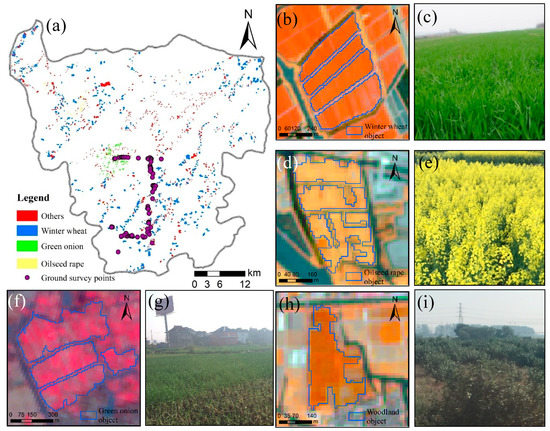
Figure 2.
Distribution of samples (a): winter wheat (b,c); oilseed rape (d,e); green onion (f,g); and woodland (h,i).
3. Methodology
The methodology employed in this study is outlined in Figure 3 and explained in detail thereafter. The eCognition software was used to perform image segmentation. The Python language together with the Geospatial Data Abstraction Library (GDAL) and Scikit-learn library were used to implement the optimal segmentation scale parameter selection, feature elimination and machine learning classification algorithms. GDAL was used to read and write the data, and Scikit-learn was used to perform the feature elimination algorithms and machine learning classification algorithms.
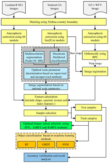
Figure 3.
Methodological workflow employed in the current study.
3.1. Image Segmentation
The eCognition software is used to segment the two Sentinel-2A images which have the highest resolution of all images used in this study. The segmentation is based on the multi-resolution segmentation algorithm, as described in [5]. In eCognition, three main parameters are supposed to be defined by users based on project requirements: the scale parameter designated as S, the shape/color parameters designated as weight wshape/wcolor and the compactness/smoothness parameters designated as weight wcompt/wsmooth. Due to fragmented and irregular croplands, the shapes of different crop fields do not differ much. Therefore, compared with shape features, we accorded more importance to the spectral features in image segmentation. As the sum of wshape and wcolor must be equal to 1.0, they were respectively set, in the current study, to 0.1 and 0.9. In a similar vein, the sum of wcompt and wsmooth must also be equal to 1.0, but in this regard, they were respectively set to 0.5 to ensure an equal importance of these parameters in image segmentation. Thus, the only parameter that needed to be optimized was scale, S.
Three regions in the test site, respectively representing areas of major winter wheat, oilseed rape and green onion cultivation were selected for acquiring the reference objects needed in determining the scale parameter (Figure 4). The first region which is predominantly of winter wheat is located in the southern part of Xinghua with an area of about 2.5 km × 1.5 km (Figure 4a). The northern part of Xinghua, composed mainly of oilseed rape, was selected as the second region with an area of about 2.1 km2 (Figure 4b). The third region consisting mainly of green was selected from the central part of Xinghua and has an area of about 2.1 km2 (Figure 4c). Both unsupervised and supervised optimal SP selection methods were employed in the current study.
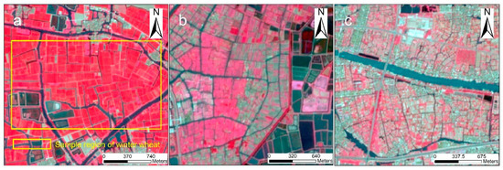
Figure 4.
Sample regions of winter wheat (a), oilseed rape (b) and green onion (c) used in determining optimal scale parameter of multi-resolution segmentation.
3.1.1. Unsupervised Optimal SP Selection Method
Espindola et al. [30] proposed an unsupervised optimal SP selection method that takes into account global intra-segment and inter-segment heterogeneity measures (weighted variance and Moran’s I, respectively) and finally obtains a global score (GS). The scale with the minimum GS is selected as the optimal SP. This method has been widely used [60,61,62] and discussed [63], and its framework is described as follows.
The global intra-segment goodness measure, weighted variance, is calculated as follows:
where n is the total number of segmentation objects; vi is the variance; and ai is the area of object i.
The inter-segment heterogeneity measure, Moran’s I, is calculated as follows:
where wij is the spatial weight between object i; and j (if they are neighbors sharing a boundary, wij = 1, otherwise, wij = 0), yi and yj are the mean spectral value of object i and j respectively, and is the mean spectral value of the image.
Then Equation (3) is used to rescale the wVar and MI to 0–1, and GS is calculated by Equation (4).
3.1.2. Supervised Optimal SP Selection Method
A supervised optimal SP selection algorithm is proposed in the current study based on the information gain ratio, which is often used in decision tree construction [48]. The detailed steps in the construction of this algorithm are described as follows:
(1) A series of SPs were used to segment the images, and then a series of segmented objects Ascale were obtained. In this study, the scales range from 10 to 180 with an interval of 10.
(2) A classification image D was obtained by visual interpretation or other classification methods. Then, H(D), which is the entropy of classification image D, was calculated using Equation (5):
where k is the number of classes in D, Pi is the probability of class i, which is the ratio of the area of class i to the total area of the image.
(3) The conditional entropy was calculated using Equation (6):
where H(D|Ascale) is the conditional entropy of image D with segmented objects and n is the total number of objects. P(A=Ai) is the probability of object i, which is calculated as the ratio of the area of object i to the total area of image D. H(D|A=Ai) is the entropy of image D within the boundary of object i and can be calculated using Equation (5).
(4) The information gain for segmented objects Ascale was defined as follows:
(5) The information gain ratio can be calculated using Equation (8). H(Ascale) is the intrinsic entropy of the segmented objects Ascale, and can be calculated using Equation (5).
With the reduction in SP, it is obvious that when the size of the segmented object is larger than the ‘real’ object (Figure 5a), the interior classes within the segmented object tend to be consistent, and the conditional entropy H(D|Ascale) will decrease while the information gain ratio gR(D,Ascale) will increase gradually together with the information gain g(D,Ascale). Once the segmentation object coincides perfectly with the actual object (Figure 5b), the information gain ratio reaches the highest point. When the segmentation object is smaller than the actual object (Figure 5c), the information gain of segmentation objects will not increase any more, but the intrinsic entropy of the segmentation objects H(Ascale) will still increase due to the increase in the number of objects, meaning the information gain ratio will decrease with the decrease in SP. Finally, the scale with the highest information gain ratio can be selected as optimal SP.
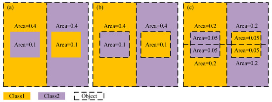
Figure 5.
Schematic diagram of changes of information gain ratio at different segmentation scales: (a) Under the condition of under-segmentation, information gain of segmentation is 0.278, the intrinsic entropy H(Ascale) is 1,and the information gain ratio is 0.278; (b) Under the condition of optimal segmentation, information gain is 1, the intrinsic entropy of segmentation objects is 1.72, and the information gain ratio increases to 0.58; (c) Under the condition of over-segmentation, information gain is still equal to 1, but the intrinsic entropy of segmentation objects increased to 2.72, and the information gain ratio decreases to 0.37.
3.2. Feature Calculation
Twelve shape features were calculated from the segmented objects, including area, length, width, compactness, density, asymmetry, roundness, elliptic fit, rectangular fit, main direction, border index and shape index.
The principal component analysis (PCA) transformation was implemented on all five images and only the first PCA of each image, which possesses the highest amount of information, was selected to calculate texture features. The 8 texture features for each image included GLCM (gray-level co-occurrence matrix) homogeneity, contrast, dissimilarity, entropy, ang.2nd moment, mean, StdDev, and correlation [64]. Thus, a total of 40 texture features were obtained for use in this study.
The spectral features included the mean and variance of each band in each image. Then a total of 76 spectral features were obtained from the 38 bands of the multisource satellite imagery.
Index features included the normalized difference vegetation index (NDVI) [65], enhanced vegetation index (EVI) [66], land surface water index (LSWI) [67], and the modified normalized difference water index (MNDWI) [68]. NDVI and EVI are the most widely used vegetation indices in remote sensing-based crop monitoring [65,66]. LSWI contains information on the moisture content of the underlying surfaces of vegetation canopies [67,69], and MNDWI presents an enhanced capability of extracting open water features as it can efficiently suppress or even remove noise from soil or built-up background [68]. Therefore, 18 index features were calculated from the five satellite images. LSWI and MNDWI were not calculated from the GF-1 WFV image due to its lack of a SWIR band.
In total, 146 features were obtained from spectra, index, shape and texture, and from which the optimal features were selected.
3.3. Optimal Feature Subset Selection
Recursive feature elimination (RFE) is an embedded backward feature elimination algorithm [54] and has been used in the selection of optimal features for use in GEOBIA. Three major steps are involved in the implementation of the RFE algorithm. Firstly, a classification model (such as RF, SVM or GBDT) is trained using training data. Secondly, all features are ranked based on their importance as generated by model training. Thirdly, the least important feature is eliminated and a new feature subset is generated. Through repetition of steps 1 to 3, the selected feature subsets are subjected to classification and accuracy assessment until the feature subset with highest classification accuracy is obtained and considered as the optimal feature subset.
Chen et al. [22] proposed an enhanced RFE (EnRFE) algorithm based on RFE. EnRFE utilizes the complete feature subset (F) and can be implemented using three major steps. Firstly, a classification model is trained using training data with features in F, and the classification accuracy of F is evaluated using testing data and all features are ranked from lowest to highest based on their importance as generated by model training. Secondly, features in F are eliminated by replacement in order of importance until a feature whose elimination will not decrease the accuracy is found. Thirdly, the second step is repeated until F attains ∅. Based on the above, the F with the highest accuracy is considered the optimal feature subset for use in subsequent tasks.
In this paper, an improved EnRFE algorithm, hereafter referred to as iEnRFE, is proposed to better select the optimal feature subset. The proposed algorithm has two major improvements relative to its precursor, EnRFE. Firstly, the iEnRFE algorithm limits the depth of feature search and the feature search changes from sequential to synchronous. This approach avoids the search for most or even the entire feature set under extreme conditions and allows for parallel computing which can greatly improve the efficiency of the algorithm. Secondly, the iEnRFE algorithm searches for d features synchronously (d is the search depth) and can ultimately find that feature whose absence would produce the highest accuracy. This eliminates the ambiguity attendant with EnRFE. The processing chain of the proposed iEnRFE algorithm is outlined in Appendix A.
3.4. Parameter Optimization of Machine-Learning Classification Algorithms for Crop Recognition
Three widely used machine-learning classifiers we reemployed for crop recognition in the current study and they include random forest (RF), gradient boosting decision tree (GBDT) and support vector machine (SVM). Parameter optimization is a crucial step for improving the performance of each classifier. In this paper, a grid search algorithm was employed to find optimal parameter values [70]. It involves an exhaustive search through a manually specified subset of the hyper parameter space of a classifier. The optimal parameter value is determined as one that produced the highest classification accuracy.
RF is a combination of many individual decision trees. Each decision tree is automatically trained based on the principle of random sampling with replacement, and the final classification result is determined by a voting process involving all decision trees [44]. There are two main parameters that need to be optimized in the RF model using grid search. They are ntree—the number of decision trees grown, and nfeature—the number of features randomly sampled as candidates at each tree node split [35]. In this study, the search range for ntree was set from 10 to 300 with an interval of 10, and that for nfeature from 5 to 30 with an interval of 5.
GBDT develops an ensemble of tree-based models by training each tree in a sequential manner [50]. Each iteration fits a decision to the residuals left by the previous and then the prediction is accomplished by combining all trees [71,72]. Learning_rate—the step size while learning, max_features—the number of features to consider when looking for the best split, and n_estimators—the number of boosting stages to perform, are the three main parameters that need to be tuned in GBDT [72]. The search range for learning_rate is was set from 0.05 to 0.3 with a search step of 0.05, that for max_features from 5 to 30 with a search step of 5, while the search range for n_estimators was set from 10 to 200 with a search step of 10.
SVM is a statistical learning model based on the principle of structural risk minimization, and looks for a hyperplane with the greatest margin to divide the samples into two classes with the largest interval [73]. When classes are not linearly separable, the kernel function of input data can be projected into a higher dimensional feature space in which data can be linearly separable [74]. SVM parameters that need optimization include kernel type, penalty parameter C, and gamma coefficient. The search values for kernel function include ‘linear’, ‘rbf’, ‘poly’ and ‘sigmoid’, those for C include 1, 2, 4, 8 and 10, and those for gamma coefficient include 0.1, 0.2, 0.5, 0.75 and 1. It should be noted that the gamma parameter is not valid for a ‘linear’ function.
In the implementation of RF, GBDT and SVM in this study, 1,418 training samples were first used to train the models. Then the trained models were used to classify the segmented objects based on the optimal feature subset. Finally, 607 test samples were used to evaluate the accuracy of crop recognition. Overall accuracy (OA), user accuracy (UA), producer accuracy (PA) and kappa coefficient were used as accuracy assessment measures [75].
4. Results and Discussion
4.1. Optimal SP Selection and Image Segmentation
Based on the supervised method proposed in Section 3.1.2, the optimal SP was calculated for the three sample regions as given in Figure 6. It is observed that the highest information gain ratios were obtained at a SP of 90 for green onion and oilseed rape, and 110 for winter wheat. Hence, based on the proposed supervised method, the optimal SP for green onion and oilseed is 90 whereas that for winter wheat is 110.
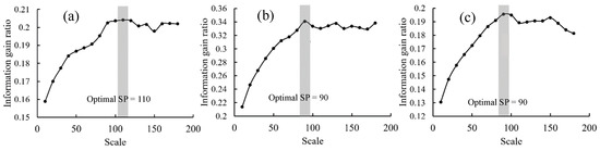
Figure 6.
Optimal scale parameters of multi-resolution segmentation selected based on information gain ratio for winter wheat (a), oilseed rape (b) and green onion (c).
Moreover, the unsupervised method described in Section 3.1.1 was also used to determine the optimal SP in the same regions as the supervised method (Figure 7). As shown in Figure 7a, intra-segment homogeneity increases with scale, indicating that the spectral difference in segmented objects decreases with the increase of scale. In Figure 7b, inter-segment heterogeneity decreases with the increase of scale, indicating that the spectral difference between segmented objects increases with scale. The scale of minimum GS in Figure 7c was selected as the optimal SP. The optimal SP of winter wheat and oilseed rape are 100, which is similar to the optimal SP selected by the supervised algorithm, and this shows the consistency between the two methods in optimal SP selection. However, the optimal SP of green onion is difficult to determine owing to a minimum GS at a scale of 150, which is obviously not the optimal SP. Moreover, GS values of green onion at scales 50 and 70 are also relatively low.
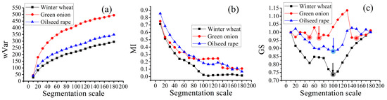
Figure 7.
Weighted variance (a), Moran’s I (b) and global score (GS) (c) changes with segmentation scale.
Based on visual interpretation, it was observed that a segmentation scale of 90 or 100 can be optimal for multi-resolution segmentation (Figure 8). A lower or higher scale parameter will result in over-segmentation or under-segmentation, respectively.
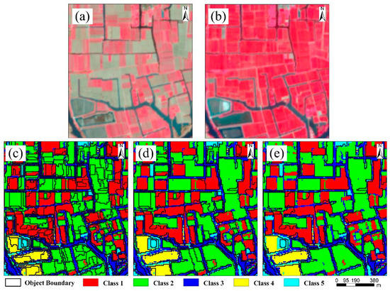
Figure 8.
Comparison of classification results and segmentation objects at different SPs: (a) False color RGB (Red/green/blue) composition of Sentinel-2A (NIR, red and green bands) on February 28, 2017; (b) false color RGB composition of Sentinel-2A (NIR, red and green bands) on April 29, 2017; (c) at a SP of 50; (d) at a SP of 90; (e) at a SP of 130.
Figure 8 shows the segmentation results of the winter wheat sample region at three different scales. It is observed that only a part of winter wheat had turned green at the end of February (Figure 8a), and in late April (Figure 8b), the entire winter wheat field had recorded substantial growth. Owing to the more obvious inter-field variability in winter wheat at the middle of the growing season, two classes were obtained from this category. Using the maximum likelihood classifier, five classes were obtained (Figure 8c–e). Each class contains pixels of similar spectra. Figure 8c shows an obvious over-segmentation at a SP of 50. Although the internal homogeneity of each object is high, the information gain ratio is low given the number of segmented objects. Figure 8e shows an obvious under-segmentation at a SP of 130. When the SP is 90, the boundaries of the segmented objects are in good agreement with the classes (Figure 8d).
Finally, 90 was selected as the optimal SP for the entire Xinghua City, given the fact that a small segmentation scale normally brings a higher classification accuracy [21]. After obtaining the optimal SP, the two Sentinel-2A images were segmented into a total number of 529,192 objects based on the multi-resolution segmentation algorithm.
It is important to note that optimal SP selection methods all have their unique advantages and disadvantages. The unsupervised optimal SP selected method has been considered as an efficient and automatic approach as it does not require the generation of reference objects, a process that can be time-consuming and subjective. However, due to the complexity and polysemy of objects, optimal SP obtained by unsupervised methods may deviate from reality (as the optimal SP of green onion in this study). Assuming crops of similar spectral patterns such as winter wheat and rapeseed coexist in a field, when the target class is cropland, a larger segmentation scale is required to combine rapeseed and winter wheat into one object, but when the target classes are winter wheat and rapeseed, a smaller SP is desirable to separate these two crops. However, optimal SP determined by unsupervised methods would not change with the target classes.
4.2. Feature Calculation and Optimal Feature Subset Selection
After extraction of image objects, a total number of 146 features, including spectral, index, shape and texture features were calculated as described in Section 3.2. Comparisons have been made in this paper among RFE, EnRFE and iEnRFE in the selection of the optimal feature subset for RF, GBDT and SVM models, and the results are presented in Figure 9.
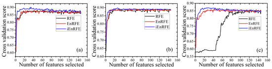
Figure 9.
Performances of the recursive feature elimination (RFE), enhanced RFE (EnRFE) and improved EnRFE (iEnRFE) algorithms based on random forest (RF) (a); gradient boosting decision tree (GBDT) (b); and support vector machine (SVM) (c) models.
It is observed that at the initial increase in the number of features, the classification accuracies of all classification methods first increase rapidly. With a further increase in the number of features, accuracies either level-off or decrease owing to the introduction of more redundant information.
It is also observed that the iEnRFE algorithm performs better in optimal feature subset selection with RF when the number of features is greater than 20 (Figure 9a). With the reduction of features, the classification accuracy of iEnRFE gradually increases, while the accuracies of RFE and EnRFE are almost stable. Figure 9b shows that the three feature selection methods have similar performances with the GBDT model, as no significant change in accuracy is observed when the number of features is greater than 20. Figure 9c shows that for the SVM model, iEnRFE obtained the highest score when the feature amount is set to 30. EnRFE also produced a higher score when the feature amount is about 30. However, when the feature amount is about 70, there is a drastic drop in the score of RFE. This phenomenon suggests that the RFE method can erroneously remove features of low importance, but which are useful to improve the overall classification accuracy when combined with other features. The iEnRFE algorithm in this regard is more effective in selecting the optimal feature subset than its precursor, EnRFE.
Table 1 shows the optimal feature subset selected for each classification model based on the iEnRFE method. It can be observed in Table 1 that index features have the highest importance amount features, accounting for 15, 13 and 14 features included in the optimal feature subsets for RF, GBDT and SVM models, respectively. The next in order of importance are spectral features, accounting for 10, 12 and 10 features in the optimal subsets for RF, GBDT and SVM models, respectively. Texture and shape features exhibited the least importance, with only of 5, 5 and 6 features being selected in the optimal subsets for RF, GBDT and SVM, respectively. This is attributable to the effect of the lower resolution images (Landsat-8) which may not have provided detailed texture and shape information that would have enhanced classification. However, texture and shape features are still useful to improve the classification accuracy.

Table 1.
Optimal feature subset for each machine learning model.
Assuming a total number of n features in the original feature subset, the time complexities of RF, EnRFE and iEnRFE were calculated. The time complexity of RFE is designated as O(n), meaning its run time will increase linearly with the increase in the number of features. The time complexity of EnRFE would reach O((n²+n)/2) at extreme conditions when it cannot find a feature whose removal would not decrease the accuracy of the feature subset, indicating that its run time will have a quadratic increase with the increase in the number of features. The time complexity of the iEnRFE is given as O(d·n), where d is a constant representing the search depth. This means that iEnRFE is a linear time algorithm as with RFE, and its computational time will not increase drastically with the number of features.
Table 2 shows the computational time of RFE, EnRFE and iEnRFE. It is observed that the computational time of EnRFE is far greater than that of RFE and iEnRFE, and this is consistent with the time complexity of the algorithm. The computational time of iEnRFE is in the same order of magnitude as the RFE algorithm. This is attributable to their similar time complexities and the parallel computing ability of the iEnRFE algorithm. The CPU of the computer used in this study has a frequency of 3.6 GHz and four cores and eight threads (Intel Core i7-7700), with a memory size of 8 GB.
Table 2.
Computational time of different feature selection algorithms based on RF, GBDT and SVM.
Overall, considering the relative efficiencies of these three algorithms, this paper proposed iEnRFE as the most appropriate algorithm, at least at present, for obtaining the optimal feature subset in the current study.
4.3. Crop Classification and Accuracy Analysis
Based on the optimal feature subset and the training data, the optimal parameter values of each machine learning model were determined through grid search. For the RF model, ntree was set to 90, and nfeature to 10. For the GBDT model, learning_rate was set to 0.1, n_estimators to 80, and max_features to 15. For the SVM model, the ‘linear’ function selected as kernel and the C parameter was set to 2, but the gamma parameter was not set as it is not required for a ‘linear’ kernel.
The RF, GBDT and SVM models were trained to classify the segmented objects. The classification results of RF, GBDT and SVM models are shown in Figure 10. From the classification results, winter wheat is the main winter crop in Xinghua and accounts for the largest share of arable land. Oilseed rape is more intensely cultivated in the northwestern part of Xinghua (Figure 10d). The area of green onion is relatively small and the crop is mostly concentrated in Duotian, in the central part of Xinghua (Figure 10e).
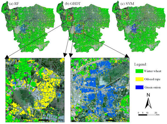
Figure 10.
Classification results of RF (a), GBDT (b), and SVM (c) models, and the main planting regions of oilseed rape (d) and green onion (e).
The accuracies of RF, GBDT and SVM were evaluated using testing data and the results are shown in Figure 11 and Appendix B. The GBDT model produced the highest overall accuracy (OA of 92.4%, with a kappa coefficient of 0.882). The RF model produced an OA of 91.8% and a kappa coefficient of 0.871, and SVM recorded the lowest accuracy among the three machine learning models, with an OA of 90.5% and a kappa coefficient of 0.853.
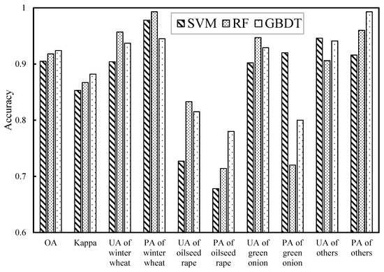
Figure 11.
Classification accuracies of RF, GBDT and SVM models.
In Figure 11, it can be observed that all the three classification methods recorded very high accuracies for winter wheat. The UA of winter wheat with RF reaches 95.1%, and the errors in this class mainly attributed to the commission of small oilseed rape parcels and wastelands that coexist with winter wheat. The PA of winter wheat with RF reaches 99.0%, meaning that almost all winter wheat farmlands were correctly classified. The good classification results of winter wheat are not unconnected to the larger parcels and more regular boundaries of this class, and these shape and textural features aided the recognition of the crop along with spectral and index features.
The accuracy of green onion is lower than that of winter wheat. SVM showed its highest accuracy with green onion, with a UA of 90.7% and a PA of 92.5%. This can be ascribed to the capability of SVM in handling small training samples [22]. The RF and GBDT models produced high UA (95.0% and 93.2%, respectively) and low PA (71.7% and 77.4%, respectively). This means that only a few pixels from other classes were misclassified into green onion, but more pixels of green onion were omitted. There are two main reasons for this phenomenon. Firstly, the planting and harvesting time of green onion varies greatly. While some green onion parcels had been harvested in April 29, thereby showing spectra similar to bare land, others were still growing vigorously. Secondly, green onion is mostly planted in the central part of Xinghua (Figure 12), where a different agricultural system is practiced [76]. This area consists of smaller parcels of crops surrounded by rivers and other water bodies (Figure 12c). The small and highly fragmented crop fields explain the obvious pixel impurity (Figure 12b) which results in the relatively low classification accuracy of green onion.
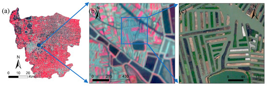
Figure 12.
Satellite image of the Duotian Agrosystem in Xinghua: (a) Sentinel image of Xinghua; (b) Sentinel image of green onion planted area; (c) high-resolution Google Earth image of green onion planted area.
With oilseed rape, all three classification methods showed lower classification accuracies. GBDT obtained the highest accuracy for oilseed rape, with a UA of 82.1% and a PA of 79.7%. There are two main reasons for this. Firstly, apart from the northwestern part of Xinghua where oilseed rape is highly concentrated, the crop is cultivated in relatively smaller parcels within and around winter wheat fields. This makes it difficult to distinguish it from winter wheat. Secondly, in northwestern Xinghua where oilseed is highly concentrated, oilseed rape is interspersed by rivers and other water bodies, and the attendant mixed-pixel effect resulted in a lower accuracy of the oilseed rape class.
The computational times of the three classification methods were recorded, and included the training time and prediction time. The results showed that the prediction times of RF, GBDT and SVM are similar, with 4.513 s, 6.849 s and 5.883 s, respectively. However, the training time of SVM is significantly more than that of RF and GBDT, with 910.415 s, 0.988 s and 3.379 s, respectively. The total time consumed by RF and GBDT is in the same order of magnitude, and because the RF algorithm has the advantage of parallel computing, its total time is less than that of GBDT. Due to the complexity of the SVM algorithm, the total computational time of SVM is much more than that of RF and GBDT. With respect to time consumed in feature selection with iEnRFE, SVM utilized more than 14 h, while RF and GBDT only utilized about 11 minutes and 8 minutes, respectively.
Considering the performances of the three methods, SVM is extremely time-consuming and has no advantage over the RF and GBDT methods in terms of classification accuracy. This suggests that for crop classification involving a large number of training samples and image features, SVM is highly inefficient. On the other hand, SVM has been known to be more efficient in crop mapping when a smaller number of training data samples is involved [77,78]. The RF and GBDT methods having recorded higher classification efficiencies and accuracies are, therefore, considered to be more suitable for use in crop recognition initiatives involving GEOBIA and multisource remote-sensing data.
It is worth noting that although the accuracy of SVM is lower than that of RF and GBDT as observed in this study, it does not suggest that SVM cannot achieve higher accuracies in other mapping scenarios. In fact, through more elaborate and complex works of sample selection, feature selection and parameter optimization, the SVM method can also obtain higher accuracies [79,80]. Besides, SVM has proved more efficient at handling small data samples, which makes it the optimal choice where the acquisition of more field data is constrained by time and resources [77,78,81].
5. Conclusions
This paper presents a complete object-based crop recognition scheme that includes the selection of the optimal SP of multi-resolution segmentation, feature subset and classification method for use in GEOBIA.
A comparison of two optimal SP selection algorithms, unsupervised and supervised, indicated that the supervised method proposed in this paper could better adapt to different situations than the unsupervised method. However, the unsupervised method proved more efficient and automatic as it does not require the acquisition of reference image objects.
Three feature selection methods including RFE, EnRFE and iEnRFE were also evaluated to arrive at the optimal subset. Results indicated that the iEnRFE algorithm proposed in this paper outperformed the preexisting RFE and EnRFE methods in selecting the optimal feature subset. Moreover, three machine-learning methods, including RF, GBDT and SVM, were used for classification, and their parameters were optimized through a grid search method. The overall accuracies of RF, GBDT and SVM were 91.8%, 92.4%, and 90.5%, respectively, indicating the feasibility of machine learning methods in obtaining accurate crop classifications based on GEOBIA and multisource satellite imagery. GBDT obtained the highest overall accuracy while utilizing the least computational time. This suggests that despite its use in crop classification not being as popular as its RF and SVM counterparts, GBDT has demonstrated a better accuracy and efficiency in crop recognition with GEOBIA and multisource satellite imagery. Additionally, despite SVM being more widely used, its huge computational time renders it less efficient especially in crop mapping initiatives that require the use of multiple sources of information and over large area. In this regard, GBDT and RF, which recorded higher accuracies with less computational time, are more suitable.
The complete object-based crop classification scheme, that includes the systematic evaluation of the optimal segmentation scale parameter, feature selection and classification algorithm, presented in this study is envisaged to provide a valuable reference for crop recognition based on GEOBIA and multisource satellite imagery. The methods proposed in this paper could also be applicable to other fields such as land-use/land-cover monitoring and change detection. However, more works are needed to evaluate the feasibility of the proposed supervised optimal SP selection and iEnRFE algorithms over large areas and in different operational scenarios. Meanwhile, the application of evolving artificial intelligence methods in crop recognition with GEOBIA is a promising scientific research direction.
Author Contributions
Conceptualization, L.Y. and J.H.; Methodology, L.Y. and J.H.; Software, L.Y.; Validation, L.Y.; Formal Analysis, L.Y., J.H. and L.W.; Investigation, L.Y., L.R.M.; Resources, J.H. and L.W.; Data Curation, L.Y.; Writing-Original Draft Preparation, L.Y. and L.R.M.; Writing-Review & Editing, L.Y., L.R.M. and J.H.; Visualization, L.Y.; Supervision, J.H.; Project Administration, J.H. and L.W.; Funding Acquisition, J.H. and L.W.
Funding
This research was funded by the Major Project for High-Resolution Earth Observation in China (grant number 09-Y20A05-9001-17/18) and Integrating Advanced Earth Observation and Environmental Information for Sustainable Management of Crop Pests and Diseases (grant number NSFC61661136004).
Acknowledgments
We thank Weiwei Liu and Huaiyue Peng of the Key Laboratory of Agricultural Remote Sensing and Information Systems of Zhejiang University, for their help in ground data collection. We also thank the anonymous reviewers for their constructive comments and advice.
Conflicts of Interest
The authors declare no conflict of interest.
Appendix A
Processing Chain of the Proposed iEnRFE Algorithm
| R: = remaining feature set which contains n features initially |
| S: = the score of a criterion function for a particular feature set, e.g. the accuracy of 4-fold cross validation |
| Sset: = the dataset which contains the scores of each iteration of R, initialize Sset = ∅ |
| k: the number of remaining features, initialize k = n |
| d: = search depth,1 < d < n |
| START: |
| Step 1: Train a model of RF, GBDT or SVM based on R, calculate the score S1 and the importance of features in R, append S1 at the end of Sset. |
| Step 2: Rank features in R based on importance from the lowest to the highest, R= {f1, f2, f3, …, fk } |
| Step 3: m = min(d, k) |
| For i = 1 to m: |
| Construct a new feature set Ri by removing the feature fi from R. |
| Train a model on the samples with the remaining features in Ri and calculate the score of Si. |
| Re-rank features in Ri based on importance from the lowest to the highest Ri = { f1, f2, f3, …, fk−1}. |
| EndFor |
| Step 4: Set Sj = max(Si), and R = Rj, k = k − 1, append Sj to the end of Sset. |
| Step 5: Repeat steps 3~4 until R = ∅ |
| Step 6: Select the feature subset R with the highest score S in Sset as the optimal feature subset |
| END. |
Appendix B
Table A1.
Error matrices of RF, GBDT and SVM methods
Table A1.
Error matrices of RF, GBDT and SVM methods
| Classification Method | Object Class | Winter Wheat | Oilseed Rape | Green Onion | Others | User’s Accuracy (%) |
|---|---|---|---|---|---|---|
| RF | Winter wheat | 193 | 5 | 0 | 5 | 95.1 |
| Oilseed rape | 0 | 49 | 3 | 7 | 83.1 | |
| Green onion | 0 | 1 | 38 | 1 | 95.0 | |
| Others | 2 | 14 | 12 | 278 | 90.8 | |
| Producer’s accuracy (%) | 99.0 | 71.0 | 71.7 | 95.5 | - | |
| Overall accuracy (%) | 91.8 | - | Kappa coefficient | 0.871 | - | |
| GBDT | Winter wheat | 192 | 4 | 1 | 9 | 93.2 |
| Oilseed rape | 0 | 55 | 4 | 8 | 82.1 | |
| Green onion | 1 | 2 | 41 | 0 | 93.2 | |
| Others | 2 | 8 | 7 | 274 | 94.2 | |
| Producer’s accuracy (%) | 98.5 | 79.7 | 77.4 | 94.1 | - | |
| Overall accuracy (%) | 92.4 | - | Kappa coefficient | 0.882 | - | |
| SVM | Winter wheat | 189 | 9 | 0 | 10 | 90.9 |
| Oilseed rape | 1 | 47 | 2 | 15 | 72.3 | |
| Green onion | 0 | 4 | 49 | 1 | 90.7 | |
| Others | 5 | 9 | 2 | 265 | 94.3 | |
| Producer’s accuracy (%) | 96.9 | 68.1 | 92.5 | 91.1 | - | |
| Overall accuracy (%) | 90.5 | - | Kappa coefficient | 0.853 | - |
References
- Godfray, H.C.; Beddington, J.R.; Crute, I.R.; Haddad, L.; Lawrence, D.; Muir, J.F.; Pretty, J.; Robinson, S.; Thomas, S.M.; Toulmin, C. Food security: The challenge of feeding 9 billion people. Science 2010, 327, 812. [Google Scholar] [CrossRef] [PubMed]
- Morton, D.C.; Defries, R.S.; Nagol, J.; Souza, C.M., Jr.; Nagol, J.; Kasischke, E.S.; Hurtt, G.C.; Dubayah, R. Mapping canopy damage from understory fires in Amazon forests using annual time series of Landsat and MODIS data. Remote Sens. Environ. 2011, 115, 1706–1720. [Google Scholar] [CrossRef]
- Mansaray, L.; Huang, W.; Zhang, D.; Huang, J.; Li, J. Mapping Rice Fields in Urban Shanghai, Southeast China, Using Sentinel-1A and Landsat 8 Datasets. Remote Sens. 2017, 9, 257. [Google Scholar] [CrossRef]
- Sharma, R.C.; Hara, K.; Tateishi, R. High-Resolution Vegetation Mapping in Japan by Combining Sentinel-2 and Landsat 8 Based Multi-Temporal Datasets through Machine Learning and Cross-Validation Approach. Land 2017, 6, 50. [Google Scholar] [CrossRef]
- Benz, U.C.; Hofmann, P.; Willhauck, G.; Lingenfelder, I.; Heynen, M. Multi-resolution, object-oriented fuzzy analysis of remote sensing data for GIS-ready information. ISPRS J. Photogramm. Remote Sens. 2004, 58, 239–258. [Google Scholar] [CrossRef]
- Novelli, A.; Aguilar, M.A.; Nemmaoui, A.; Aguilar, F.J.; Tarantino, E. Performance evaluation of object based greenhouse detection from Sentinel-2 MSI and Landsat 8 OLI data: A case study from Almeria (Spain). Int. J. Appl. Earth Obs. 2016, 52, 403–411. [Google Scholar] [CrossRef]
- Zhou, W.Q.; Huang, G.L.; Troy, A.; Cadenasso, M.L. Object-based land cover classification of shaded areas in high spatial resolution imagery of urban areas: A comparison study. Remote Sens. Environ. 2009, 113, 1769–1777. [Google Scholar] [CrossRef]
- Amani, M.; Salehi, B.; Mahdavi, S.; Granger, J.; Brisco, B. Wetland classification in Newfoundland and Labrador using multi-source SAR and optical data integration. GISci. Remote Sens. 2017, 54, 779–796. [Google Scholar] [CrossRef]
- Kussul, N.; Lemoine, G.; Gallego, F.J.; Skakun, S.V. Parcel-Based Crop Classification in Ukraine Using Landsat-8 Data and Sentinel-1A Data. IEEE J. Sel. Top. Appl. Earth Observ. Remote Sens. 2017, 9, 2500–2508. [Google Scholar] [CrossRef]
- Myint, S.W.; Gober, P.; Brazel, A.; Grossman-Clarke, S.; Weng, Q. Per-pixel vs. object-based classification of urban land cover extraction using high spatial resolution imagery. Remote Sens. Environ. 2011, 115, 1145–1161. [Google Scholar] [CrossRef]
- Drăguţ, L.; Blaschke, T. Automated classification of landform elements using object-based image analysis. Geomorphology 2006, 81, 330–344. [Google Scholar] [CrossRef]
- Wang, L.; Sousa, W.P.; Gong, P. Integration of object-based and pixel-based classification for mapping mangroves with IKONOS imagery. Int. J. Remote Sens. 2004, 25, 5655–5668. [Google Scholar] [CrossRef]
- Jobin, B.; Labrecque, S.; Grenier, M.; Falardeau, G. Object-Based Classification as an Alternative Approach to the Traditional Pixel-Based Classification to Identify Potential Habitat of the Grasshopper Sparrow. Environ. Manag. 2008, 41, 20–31. [Google Scholar] [CrossRef] [PubMed]
- Byun, Y.G. A multispectral image segmentation approach for object-based image classification of high resolution satellite imagery. KSCE J. Civ. Eng. 2013, 17, 486–497. [Google Scholar] [CrossRef]
- Coillie, F.M.B.V.; Verbeke, L.P.C.; Wulf, R.R.D. Feature selection by genetic algorithms in object-based classification of IKONOS imagery for forest mapping in Flanders, Belgium. Remote Sens. Environ. 2007, 110, 476–487. [Google Scholar]
- Huang, Y.; Zhao, C.; Yang, H.; Song, X.; Chen, J.; Li, Z. Feature Selection Solution with High Dimensionality and Low-Sample Size for Land Cover Classification in Object-Based Image Analysis. Remote Sens. 2017, 9, 939. [Google Scholar] [CrossRef]
- Kavzoglu, T.; Colkesen, I.; Yomralioglu, T. Object-based classification with rotation forest ensemble learning algorithm using very-high-resolution WorldView-2 image. Remote Sens. Lett. 2015, 6, 834–843. [Google Scholar] [CrossRef]
- Cánovasgarcía, F.; Alonsosarría, F. Optimal Combination of Classification Algorithms and Feature Ranking Methods for Object-Based Classification of Submeter Resolution Z/I-Imaging DMC Imagery. Remote Sens. 2015, 7, 4651–4677. [Google Scholar] [CrossRef]
- Zhang, L.; Jia, K.; Li, X.; Yuan, Q.; Zhao, X. Multi-scale segmentation approach for object-based land-cover classification using high-resolution imagery. Remote Sens. Lett. 2014, 5, 73–82. [Google Scholar] [CrossRef]
- Liu, D.; Xia, F. Assessing object-based classification: Advantages and limitations. Remote Sens. Lett. 2009, 1, 187–194. [Google Scholar] [CrossRef]
- Ma, L.; Cheng, L.; Li, M.; Liu, Y.; Ma, X. Training set size, scale, and features in Geographic Object-Based Image Analysis of very high resolution unmanned aerial vehicle imagery. ISPRS J. Photogramm. Remote Sens. 2015, 102, 14–27. [Google Scholar] [CrossRef]
- Chen, X.W.; Jeong, J.C. Enhanced Recursive Feature Elimination. In Proceedings of the International Conference on Machine Learning and Applications, Cincinnati, OH, USA, 13–15 December 2007; pp. 429–435. [Google Scholar]
- Laliberte, A.S.; Browning, D.M.; Rango, A. A comparison of three feature selection methods for object-based classification of sub-decimeter resolution UltraCam-L imagery. Int. J. Appl. Earth Observ. Geoinf. 2012, 15, 70–78. [Google Scholar] [CrossRef]
- Li, L.; Solana, C.; Canters, F.; Kervyn, M. Testing random forest classification for identifying lava flows and mapping age groups on a single Landsat 8 image. J. Volcanol. Geotherm. Res. 2017, 345, 109–124. [Google Scholar] [CrossRef]
- Buddhiraju, K.M.; Rizvi, I.A. Comparison of CBF, ANN and SVM classifiers for object based classification of high resolution satellite images. In Proceedings of the Geoscience and Remote Sensing Symposium, Honolulu, HI, USA, 25–30 July 2010; pp. 40–43. [Google Scholar]
- Bhaskaran, S.; Paramananda, S.; Ramnarayan, M. Per-pixel and object-oriented classification methods for mapping urban features using Ikonos satellite data. Appl. Geogr. 2010, 30, 650–665. [Google Scholar] [CrossRef]
- Laliberte, A.S.; Rango, A.; Havstad, K.M.; Paris, J.F.; Beck, R.F.; Mcneely, R.; Gonzalez, A.L. Object-oriented image analysis for mapping shrub encroachment from 1937 to 2003 in southern New Mexico. Remote Sens. Environ. 2004, 93, 198–210. [Google Scholar] [CrossRef]
- Kim, M.; Madden, M.; Warner, T. Estimation of optimal image object size for the segmentation of forest stands with multispectral IKONOS imagery. In Object-Based Image Analysis; Springer: Berlin/Heidelberg, Germany, 2008; pp. 291–307. [Google Scholar]
- Rau, J.Y.; Jhan, J.P.; Rau, R.J. Semiautomatic Object-Oriented Landslide Recognition Scheme From Multisensor Optical Imagery and DEM. IEEE Trans. Geosci. Remote Sens. 2013, 52, 1336–1349. [Google Scholar] [CrossRef]
- Espindola, G.M.; Camara, G.; Reis, I.A.; Bins, L.S.; Monteiro, A.M. Parameter selection for region-growing image segmentation algorithms using spatial autocorrelation. Int. J. Remote Sens. 2006, 27, 3035–3040. [Google Scholar] [CrossRef]
- Möller, M.; Lymburner, L.; Volk, M. The comparison index: A tool for assessing the accuracy of image segmentation. Int. J. Appl. Earth Observ. Geoinf. 2007, 9, 311–321. [Google Scholar] [CrossRef]
- Clinton, N.; Holt, A.; Scarborough, J.; Yan, L.; Gong, P. Accuracy Assessment Measures for Object-based Image Segmentation Goodness. Photogramm. Eng. Remote Sens. 2010, 76, 289–299. [Google Scholar] [CrossRef]
- Gao, H.; Tang, Y.; Jing, L.; Li, H.; Ding, H. A Novel Unsupervised Segmentation Quality Evaluation Method for Remote Sensing Images. Sensors 2017, 17, 2427. [Google Scholar] [CrossRef] [PubMed]
- Kalantar, B.; Mansor, S.B.; Sameen, M.I.; Pradhan, B.; Shafri, H.Z.M. Drone-based land-cover mapping using a fuzzy unordered rule induction algorithm integrated into object-based image analysis. Int. J. Remote Sens. 2017, 38, 2535–2556. [Google Scholar] [CrossRef]
- Mellor, A.; Haywood, A.; Jones, S.; Wilkes, P. Forest Classification using Random forests with multisource remote sensing and ancillary GIS data. In Proceedings of the Australian Remote Sensing and Photogrammetry Conference, Melbourne, Australia, 27–28 August 2012. [Google Scholar]
- Costa, H.; Foody, G.M.; Boyd, D.S. Supervised methods of image segmentation accuracy assessment in land cover mapping. Remote Sens. Environ. 2018, 205, 338–351. [Google Scholar] [CrossRef]
- Zhang, H.; Fritts, J.E.; Goldman, S.A. Image segmentation evaluation: A survey of unsupervised methods. Comput. Vis. Image Understand. 2008, 110, 260–280. [Google Scholar] [CrossRef]
- Kaya, G.T.; Torun, Y.; Küçük, C. Recursive feature selection based on non-parallel SVMs and its application to hyperspectral image classification. In Proceedings of the Geoscience and Remote Sensing Symposium, Quebec City, QC, Canada, 13–18 July 2014; pp. 3558–3561. [Google Scholar]
- Cintra, M.E.; Camargo, H.A. Feature Subset Selection for Fuzzy Classification Methods; Springer: Berlin/Heidelberg, Germany, 2010; pp. 318–327. [Google Scholar]
- Han, Y.; Yu, L. A Variance Reduction Framework for Stable Feature Selection. Stat. Anal. Data Min. 2012, 5, 428–445. [Google Scholar] [CrossRef]
- Khair, N.M.; Hariharan, M.; Yaacob, S.; Basah, S.N. Locality sensitivity discriminant analysis-based feature ranking of humanemotion actions recognition. J. Phys. Therapy Sci. 2015, 27, 2649–2653. [Google Scholar] [CrossRef] [PubMed][Green Version]
- Wu, B.; Chen, C.; Kechadi, T.M.; Sun, L. comparative evaluation of filter-based feature selection methods for hyper-spectral band selection. Int. J. Remote Sens. 2013, 34, 7974–7990. [Google Scholar] [CrossRef]
- Mursalin, M.; Zhang, Y.; Chen, Y.; Chawla, N.V. Automated Epileptic Seizure Detection Using Improved Correlation-based Feature Selection with Random Forest Classifier. Neurocomputing 2017, 241, 204–214. [Google Scholar] [CrossRef]
- Breiman, L. Random Forests. Mach. Learn. 2001, 45, 5–32. [Google Scholar] [CrossRef]
- Chang, C.; Lin, C. LIBSVM: A library for support vector machines. ACM Trans. Intel. Syst. Technol. 2011, 2, 27. [Google Scholar] [CrossRef]
- Guyon, I.; Elisseeff, A. An introduction to variable and feature selection. J. Mach. Learn. Res. 2003, 3, 1157–1182. [Google Scholar]
- Guyon, I. Erratum: Gene selection for cancer classification using support vector machines. Mach. Learn. 2001, 46, 389–422. [Google Scholar] [CrossRef]
- Quinlan, J.R. C4. 5: Programs for Machine Learning; Elsevier: Amsterdam, The Netherlands, 2014. [Google Scholar]
- Breiman, L.; Friedman, J.H.; Olshen, R.; Stone, C.J. Classification and Regression Trees. Encycl. Ecol. 1984, 57, 582–588. [Google Scholar]
- Friedman, J.H. Greedy function approximation: A gradient boosting machine. Ann. Stat. 2001, 29, 1189–1232. [Google Scholar] [CrossRef]
- Duro, D.C.; Franklin, S.E.; Dubé, M.G. A comparison of pixel-based and object-based image analysis with selected machine learning algorithms for the classification of agricultural landscapes using SPOT-5 HRG imagery. Remote Sens. Environ. 2012, 118, 259–272. [Google Scholar] [CrossRef]
- Liu, T.; Abdelrahman, A. An Object-Based Image Analysis Method for Enhancing Classification of Land Covers Using Fully Convolutional Networks and Multi-View Images of Small Unmanned Aerial System. Remote Sens. 2018, 10, 457. [Google Scholar] [CrossRef]
- Ma, L.; Fu, T.; Blaschke, T.; Li, M.; Tiede, D.; Zhou, Z.; Ma, X.; Chen, D. Evaluation of Feature Selection Methods for Object-Based Land Cover Mapping of Unmanned Aerial Vehicle Imagery Using Random Forest and Support Vector Machine Classifiers. ISPRS Int. J. Geo-Inf. 2017, 6, 51. [Google Scholar] [CrossRef]
- Guyon, I.; Weston, J.; Barnhill, S.; Vapnik, V. Gene Selection for Cancer Classification using Support Vector Machines. Mach. Learn. 2002, 46, 389–422. [Google Scholar] [CrossRef]
- Li, W.; Li, H.; Wang, J.; Huang, W. A study on classification and monitoring of winter wheat growth status by Landsat/TM image. J. Triticeae Crops 2010, 30, 92–95. [Google Scholar]
- Liu, J.; Zhu, W.; Sun, G.; Zhang, J.; Jiang, N. Endmember abundance calibration method for paddy rice area extraction from MODIS data based on independent component analysis. Trans. Chin. Soc. Agric. Eng. 2012, 28, 103–108. [Google Scholar]
- Xue, Y.; Li, J. Year-round production technology of green onion in Xinhua. Shanghai Vegetables 2012, 6, 28–29. [Google Scholar]
- Vermote, E.F.; Tanre, D.; Deuze, J.L.; Herman, M. Second Simulation of the Satellite Signal in the Solar Spectrum, 6S: An overview. Geosci. Remote Sens. IEEE Trans. 2002, 35, 675–686. [Google Scholar] [CrossRef]
- Liu, J.; Wang, L.; Yang, L.; Shao, J.; Teng, F.; Yang, F.; Fu, C. Geometric correction of GF-1 satellite images based on block adjustment of rational polynomial model. Trans. Chin. Soc. Agric. Eng. 2015, 31, 146–154. [Google Scholar]
- Martha, T.R.; Kerle, N.; Westen, C.J.V.; Jetten, V.; Kumar, K.V. Segment Optimization and Data-Driven Thresholding for Knowledge-Based Landslide Detection by Object-Based Image Analysis. IEEE Trans. Geosci. Remote Sens. 2011, 49, 4928–4943. [Google Scholar] [CrossRef]
- Zhang, C.; Xie, Z. Combining object-based texture measures with a neural network for vegetation mapping in the Everglades from hyperspectral imagery. Remote Sens. Environ. 2012, 124, 310–320. [Google Scholar] [CrossRef]
- Johnson, B.; Xie, Z. Unsupervised image segmentation evaluation and refinement using a multi-scale approach. Isprs J. Photogramm. Remote Sens. 2011, 66, 473–483. [Google Scholar] [CrossRef]
- Böck, S.; Immitzer, M.; Atzberger, C. On the objectivity of the objective function—Problems with unsupervised segmentation evaluation based on global score and a possible remedy. Remote Sens. 2017, 9, 769. [Google Scholar] [CrossRef]
- Haralick, R.M.; Shanmugam, K.; Dinstein, I. Textural Features for Image Classification. Syst. Man Cybern. IEEE Trans. 1973, 6, 610–621. [Google Scholar] [CrossRef]
- Rouse, J.W.J.; Haas, R.H.; Schell, J.A.; Deering, D.W. Monitoring Vegetation Systems in the Great Plains with Erts. NASA Spec. Publ. 1974, 351, 309. [Google Scholar]
- Huete, A.; Justice, C.; Liu, H. Development of vegetation and soil indices for MODIS-EOS. Remote Sens. Environ. 1994, 49, 224–234. [Google Scholar] [CrossRef]
- Gao, B.C. NDWI—A normalized difference water index for remote sensing of vegetation liquid water from space. Remote Sens. Environ. 1996, 58, 257–266. [Google Scholar] [CrossRef]
- Xu, H. Modification of normalised difference water index (NDWI) to enhance open water features in remotely sensed imagery. Int. J. Remote Sens. 2006, 27, 3025–3033. [Google Scholar] [CrossRef]
- Jurgens, C. The modified normalized difference vegetation index (mNDVI) a new index to determine frost damages in agriculture based on Landsat TM data. Int. J. Remote Sens. 1997, 18, 3583–3594. [Google Scholar] [CrossRef]
- Reif, M.; Shafait, F.; Dengel, A. Meta-Learning for Evolutionary Parameter Optimization of Classifiers. Mach. Learn. 2012, 87, 357–380. [Google Scholar] [CrossRef]
- Chopra, T.; Vajpai, J. Fault Diagnosis in Benchmark Process Control System Using Stochastic Gradient Boosted Decision Trees. Int. J. Soft Comput. Eng. 2011, 1, 98–101. [Google Scholar]
- Liu, L.; Ji, M.; Buchroithner, M. Combining Partial Least Squares and the Gradient-Boosting Method for Soil Property Retrieval Using Visible Near-Infrared Shortwave Infrared Spectra. Remote Sens. 2017, 9, 1299. [Google Scholar] [CrossRef]
- Cherkassky, V. The nature of statistical learning theory. IEEE Trans. Neural Netw. 2002, 38, 409. [Google Scholar] [CrossRef] [PubMed]
- Qi, H.N.; Yang, J.G.; Zhong, Y.W.; Deng, C. Multi-class SVM based remote sensing image classification and its semi-supervised improvement scheme. In Proceedings of the International Conference on Machine Learning and Cybernetics, Shanghai, China, 26–29 August 2004; pp. 3146–3151. [Google Scholar]
- HAY, A.M. The derivation of global estimates from a confusion matrix. Int. J. Remote Sens. 1988, 9, 1395–1398. [Google Scholar] [CrossRef]
- Bai, Y.; Sun, X.; Tian, M.; Fuller, A.M. Typical Water-Land Utilization GIAHS in Low-Lying Areas: The Xinghua Duotian Agrosystem Example in China. J. Resour. Ecol. 2014, 5, 320–327. [Google Scholar]
- Chi, M.; Rui, F.; Bruzzone, L. Classification of hyperspectral remote-sensing data with primal SVM for small-sized training dataset problem. Adv. Space Res. 2008, 41, 1793–1799. [Google Scholar] [CrossRef]
- Yu, Y.; McKelvey, T.; Kung, S. A classification scheme for ‘high-dimensional-small-sample-size’ data using soda and ridge-SVM with microwave measurement applications. In Proceedings of the 2013 IEEE International Conference on Acoustics, Speech and Signal Processing (ICASSP), Vancouver, BC, Canada, 26–31 May 2013; pp. 3542–3546. [Google Scholar]
- Samadzadegan, F.; Hasani, H.; Schenk, T. Simultaneous feature selection and SVM parameter determination in classification of hyperspectral imagery using Ant Colony Optimization. Can. J. Remote Sens. 2012, 38, 139–156. [Google Scholar] [CrossRef]
- Mao, Q.H.; Ma, H.W.; Zhang, X.H. SVM Classification Model Parameters Optimized by Improved Genetic Algorithm. Adv. Mater. Res. 2014, 889–890, 617–621. [Google Scholar] [CrossRef]
- Poursanidis, D.; Topouzelis, K.; Chrysoulakis, N. Mapping coastal marine habitats and delineating the deep limits of the Neptune’s seagrass meadows using very high resolution Earth observation data. Int. J. Remote Sens. 2018, 39, 8670–8687. [Google Scholar] [CrossRef]


© 2019 by the authors. Licensee MDPI, Basel, Switzerland. This article is an open access article distributed under the terms and conditions of the Creative Commons Attribution (CC BY) license (http://creativecommons.org/licenses/by/4.0/).