Article

Rubber Identification Based on Blended High Spatio-Temporal Resolution Optical Remote Sensing Data: A Case Study in Xishuangbanna

1
College of Tourism & Geography Science, Yunnan Normal University, Kunming 650500, China
2
Provincial Key Laboratory of Plateau Geographical Processes & Environmental Change, Kunming 650500, China
3
Faculty of Geographical Science, Beijing Normal University, Beijing 100875, China
4
State Key Laboratory of Remote Sensing Science, Faculty of Geographical Science, Beijing Normal University, Beijing 100875, China
*
Authors to whom correspondence should be addressed.
Remote Sens. 2019, 11(5), 496; https://doi.org/10.3390/rs11050496
Submission received: 31 January 2019 / Revised: 20 February 2019 / Accepted: 25 February 2019 / Published: 1 March 2019
(This article belongs to the Special Issue Multitemporal Remote Sensing for Forestry)

Abstract

:
As an important economic resource, rubber has rapidly grown in Xishuangbanna of Yunnan Province, China, since the 1990s. Tropical rainforests have been replaced by extensive rubber plantations, which has resulted in ecological problems such as the loss of biodiversity and local water shortages. It is vitally important to accurately map the rubber plantations in this region. Although several rubber mapping methods have been proposed, few studies have investigated methods based on optical remote sensing time series data with high spatio-temporal resolution due to the cloudy and foggy weather conditions in this area. This study presented a rubber plantation identification method that used spatio-temporal optical remote sensing data fusion technology to obtain vegetation index data at high spatio-temporal resolution within the optical remote sensing window in Xishuangbanna. The analysis of the proposed method shows that (1) fused optical remote sensing data with high spatio-temporal resolution could map the rubber distribution with high accuracy (overall accuracy of up to 89.51% and kappa of 0.86). (2) Fused indices have high R2 (R2 greater than 0.8, where R is the correlation coefficient) with the indices that were derived from the Landsat observed data, which indicates that fusion results are dependable. However, the fusion accuracy is affected by terrain factors including elevation, slope, and slope aspects. These factors have obvious negative effects on the fusion accuracy of high spatio-temporal resolution optical remote sensing data: the highest fusion accuracy occurred in areas with elevations between 1201 and 1400 m.a.s.l., and the lowest accuracy occurred in areas with elevations less than 600 m.a.s.l. For the 5 fused time series indices (normalized difference vegetation index (NDVI), enhanced vegetation index (EVI), normalized difference moisture index (NDMI), normalized burn ratio (NBR), and tasseled cap angle (TCA)), the fusion accuracy decreased with increasing slope, and increasing slope had the least impact on the EVI, but the greatest negative impact on the NDVI; the slope aspect had a limited influence on the fusion accuracies of the 5 time series indices, but fusion accuracy was lowest on the northwest slope. (3) EVI had the highest accuracy of rubber plantation classification among the 5 time series indices, and the overall classification accuracies of the time series EVI for the four different years (2000, 2005, 2010, and 2015) reached 87.20% (kappa 0.82), 86.91% (kappa 0.81), 88.85% (kappa 0.84), and 89.51% (kappa 0.86), respectively. The results indicate that the method is a promising approach for rubber plantation mapping and the detection of changes in rubber plantations in this tropical area.

Graphical Abstract

1. Introduction

Due to an increase in the concern regarding natural forest management and conservation, the rubber plantations in Xishuangbanna have gained worldwide attention [1,2]. Since the 1990s, rubber trees planted in this area have expanded rapidly due to the increasing price of rubber. As reported by a recent study, rubber plantations are being pushed to higher elevations (approximately 1400 m.a.s.l. in 2010) in Xishuangbanna, China [3]. The rubber planting area in Yunnan Province (approximately 0.571 million ha.) exceeded that in Hainan (approximately 0.542 million ha.) and became the largest rubber plating area in China in 2015 [4]. Xishuangbanna contains 75% of the rubber plantations in Yunnan [5], and so therefore detailed, accurate, and timely mapping of the rubber plantations in Xishuangbanna is vitally important to satisfy the demands of rubber growers, marketers, and policymakers.
There are several methods to map rubber plantations. However, the defoliation of rubber trees during winter is a unique phenomenon for the vegetation in subtropical areas, and this phenomenon can be remotely sensed by using both optical and SAR (synthetic aperture radar) data. Consequently, phenological feature-based methods are the most commonly used methods [6,7]. According to the remote sensing data used, phenological feature-based rubber classification methods can be classified into two categories: methods that utilize SAR data and those that utilize optical remote sensing images. For the methods that utilize optical remote sensing images, the specific reflectance of monoculture rubber plantations and their changes could be captured by high revisit frequency remote sensors, such as MODIS (MODerate-resolution Imaging Spectroradiometer) and AVHRR (Advanced Very High Resolution Radiometer) [8,9]. However, the relatively coarse spatial resolutions of these time series data make it difficult to delineate and map rubber plantations in fragmented landscapes in tropical regions with high accuracy [7]. Studies have demonstrated the promising utility of optical remote sensing data with high temporal resolution for differentiating rubber trees from other vegetation [10]. It is even possible to map the age of a rubber plantation in Xishuangbanna using aggregated Landsat TM (Thematic Mapper) and ETM+ (Enhanced Thematic Mapper Plus) images [11,12,13]. The object-level phenological features of a rubber plantation captured by Landsat NDVI data with 30 m spatial resolution were proven to be better than pixel-based rubber classifications [14]. However, rubber trees in Xishuangbanna are planted on slopes with complex vegetation species. Considering the fragmented landscape and complex vegetation planting structure that may give rise to mixed pixels, it is challenging to use phenological features derived from time series optical satellite images with coarse spatial resolution to delineate and map the rubber plantations in this subtropical region [6,15]. Aerial photography and low-altitude sensing platforms (such as unmanned aerial vehicles, and maned airplane, balloon) can provide high-resolution data [16,17], but their endurance limits their applications in the identification of rubber plantations for larger areas. Another constraint for land cover classification in tropical areas is the frequent presence of clouds and fog cover, which makes it difficult to construct continuous mid- or high-resolution time series data with reliable quality [18]. Although the approach presented by [19] can monitor the expansion of rubber plantations by detecting and analyzing the shapelet structure in a Landsat-NDVI time series, and this method was proven to work well for the non-defoliation rubber identification, the 16-day revisit cycle and heavy cloud (and fog) contamination to optical remote sensing images remains a challenge for Landsat data to capture the accurate phenological change to identify defoliate rubber. Thus, a further study on using dense Landsat-like data to identify defoliation rubber is still missing.
In comparison to optical sensors, SAR can penetrate clouds and fog, and thus has advantages when mapping tropical forests. B. Chen integrated SAR and multitemporal Landsat imagery to extract the rubber plantations on Hainan Island of China, and the results demonstrated a great potential of using SAR data to map rubber plantations with high accuracy [18]. Another strategy used SAR data to identify forests according to the different HH (Horizontal transmitting and Horizontal receiving) and HV (Horizontal transmitting and Vertical receiving) polarizations between forest and other vegetation types. The forest areas were then classified into rubber trees and other tree types following the phenological features derived from time series vegetation indices (such as NDVI, EVI, LSWI (land surface water index), and LAI (leaf area index)). These indices are commonly calculated using optical images such as MODIS, Landsat, or HJ-1A/B [9,20,21]. Although SAR data are promising for the continuous acquisition of data in this frequently fog or cloud covered area, the fusion of optical data and SAR data, as well as the rugged terrain, remain obstacles to the rubber classification methods that utilize SAR data.
As the methods that utilized SAR and optical data presented promising results in terms of rubber classification, methods that integrate data from multiple sensors could be used to derive phenological and spectral reflectance features from vegetation, which would improve the accuracy of rubber identification [22]. Other constraints to rubber classification in Xishuangbanna are terrain characteristics such as slope, aspect, and elevation [14]. With the development of high spatio-temporal resolution optical data fusion algorithms, it is feasible to construct high spatio-temporal resolution optical data to identify rubbers [23,24]. Thus, this paper aims to blend high spatio-temporal resolution optical data using Landsat and MODIS data, and 5 indices (NDVI, EVI, NDMI, NBR, and TCA) will be derived based on this blended data set. Each of these indices will be used to classify rubbers to analyze how the terrain factors (TFs) affect the accuracy of rubber identification in Xishuangbanna and determine which of the blended high spatio-temporal indices would be the optimum choice for rubber classification.
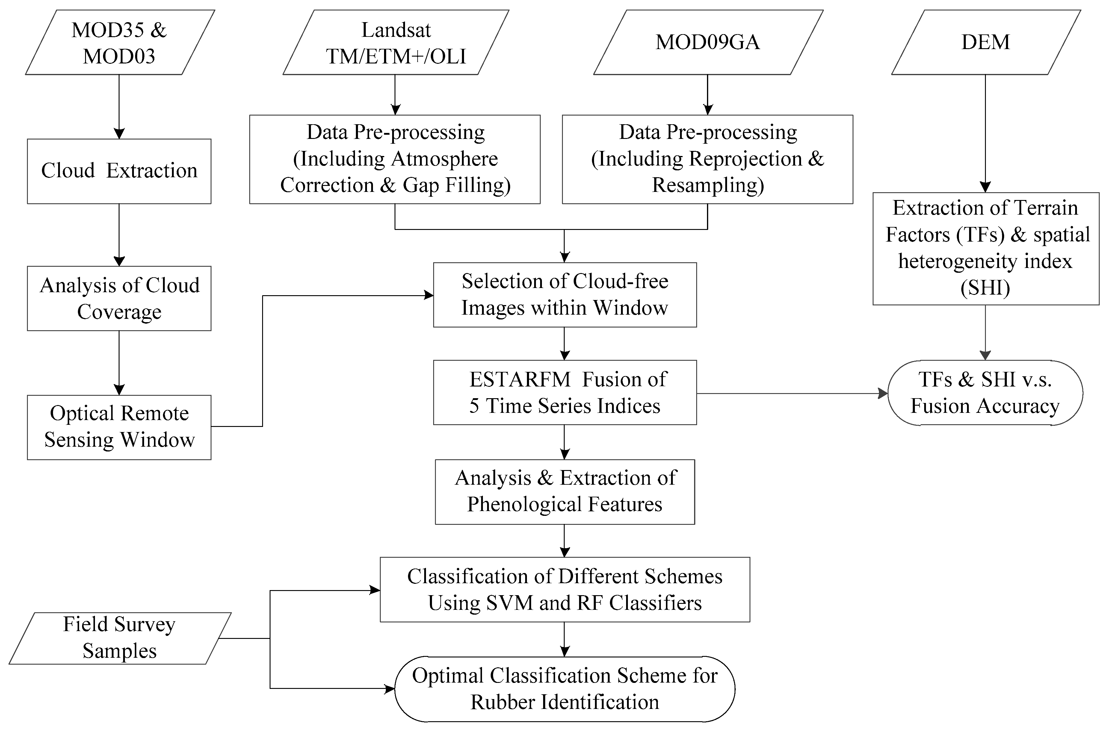
2. Study Area and Data

2.1. Study Area

The study area was located in Xishuangbanna at the southern tip of Yunnan Province, China (21°08′N~22°36′N, 99°56′E~101°51′E), and the Landsat footprint WRS-2 path 130, row 45 covers approximately 90% of this area. Xishuangbanna is in a tropical monsoon climate region where there are only two seasons: the wet season and the dry season. The wet season lasts from May to October, and the dry season lasts from November to April of the following year. Cloudy and foggy weather frequently occur in Xishuangbanna throughout the year. Xishuangbanna is a mountainous area with the lowest elevation at 470 m.a.s.l. and the highest elevation at 2429 m.a.s.l. Segmented by rugged terrain, heterogeneous land surfaces are the common feature of this area.
Driven by the increasing demand and price of rubber, the rubber plantations in China have rapidly expanded in recent decades. China began to plant rubber over large areas in Xishuangbanna in 1952, and Xishuangbanna currently contains the largest rubber planting area in Yunnan, accounting for approximately 75% of the rubber plantation area in the province. The most recent intensively rubber planting occurred in 2000 (during the China and Association of South East Asian Nations established cooperation) and 2010 (when the China-ASEAN Free Trade Zone was officially launched) [15].

2.2. Data

2.2.1. Remote Sensing Data

MODIS products with high revisit frequencies such as MOD03 (daily latitude and longitude coordinate product), MOD035 level 2 data (daily 1 km spatial resolution MODIS cloud mask and spectral test results product), and MOD09GA (daily 500 m resolution MODIS surface reflectance product) were used in this study. These data were downloaded from the NASA data sharing platform (http://reverb.echo.nasa.gov/). The combination of MOD03 and MOD035 data was used to extract cloud cover during the periods of 2000, 2005, 2010, and 2015. The data were chosen from DOY 152 (DOY, day of year) to DOY 152 of the following year because this period covers the entire dry season in Xishuangbanna. The MOD09GA data were chosen according to available Landsat data; for example, MOD09GA daily data were chosen from DOY 306 of 2000 to DOY 052 of 2001, as there were three Landsat images available from DOY 306 of 2000 to DOY 052 of 2001 during the dry season of 2000. Each MODIS product was reprojected from its original coordinate system to Universal Transverse Mercator (UTM) coordinates with the WGS84 datum by applying the MODIS Reprojection Tools (MRT, available from https://lpdaac.usgs.gov/tools/modis_reprojection_tool).
The 30 m spatial resolution cloud-free Landsat TM/ETM+/OLI (Operational Land Imager) data were downloaded from the USGS Land Processes Distributed Active Archive Center (http://glovis.usgs.gov/). The spectral response characteristics of the Landsat series data are consistent, and thus, the vegetation index calculated from different Landsat sensors have no significant deviations, which means the uncertainty caused by combined usage of different Landsat sensors to derive vegetation indices will have negligible effects on the fusion results. The Landsat image with a scene path of 130, row 45 was chosen for each of the four periods (the years of 2000, 2005, 2010, and 2015). There were at least three clear Landsat images for each period. Due to the failure of the scan-line corrector (SLC), approximately 22% of the pixels are unscanned in each ETM+ image, so this study utilized the GNSPI (geostatistical neighborhood similar pixel interpolator) algorithm to fill the gaps of the ETM+ SLC-off images, an algorithm based on the geostatistical theory; compared with previous methods, the image filled by GNSPI has fewer striping effects [25]. For the atmosphere correction of Landsat data, the Landsat ecosystem disturbance adaptive processing system (LEDAPS), which is based on a large number of observed aerosol data and following the 6S model, which processes Landsat imagery to surface reflectance based on the Second Simulation of a Satellite Signal in the Solar Spectrum radiative-transfer model (6S model) used by MODIS land science team [26], was used to create the Landsat-based surface reflectance data. Considering the small portion of cloud coverage in the selected data, the Fmask algorithm provided by Zhu was used to remove the clouded and shadowed pixels, and the removed pixels were filled with the nearest available data [27]. In addition, a digital elevation model (DEM) was also used. The data were downloaded from the GDEM (global digital elevation model, http://gdem.ersdac.jspacesystems.or.jp/) in the WGS-84 coordinate system at 30 m spatial resolution. The GDEM data were used to extract the slope, aspect, and elevation to analyze their impacts on the rubber identification results. See Table 1:

2.2.2. Field Data

Intensive field surveys were launched from 2015 to 2018 in Xishuangbanna, and each field survey was during (or near) the dry season to ensure that limited land cover change occurred between the survey and the nearest available satellite image. The distribution of the survey points and the field survey routes are shown in Figure 1. The field investigation was intensified in areas where the land cover distribution was fragmented, and 7 main land cover types (namely, road, buildings, water body, grass land, crops, forest and others) were covered in the field survey. Detailed investigations of crops and forest were conducted because these two cover types in Xishuangbanna have changed dramatically in recent decades. We first divided the land cover into vegetation and non-vegetation. Then, crops such as paddy field and dry land were investigated, and vegetation areas were divided into natural forest, rubber, and other planted vegetation (such as farmland, eucalyptus, and tea plants). To meet the demands for rubber classification in this study, we reclassified the field survey points into 4 classes: natural forest, rubber plantations, other vegetation, and non-vegetation cover, as described in detail in Table 2. For the years of 2005, 2010, and 2015, Google Earth images with high spatial resolution were used to establish remote sensing samples for each of the 4 types of land cover. For the year of 2000, because of the lack of Google Earth images with high spatial resolution in our study area, a SPOT-2 image (acquired on DOY 053 of 2001) at 10 m spatial resolution was used to assist with the selection of samples. In our study area, a total of 600 sample points of different land cover types were selected for the 4 chosen periods (250 natural forest, 170 rubber plantations, 100 other vegetation, and 80 non-vegetation). Samples were selected based on a stratified random sampling method [28,29]; 1/3 of the samples were selected as training samples, and the remaining 2/3 of the samples were used as validation samples to assess the classification results.

2.2.3. Construction of Time Series Indices

Considering the complex landscape characteristics of Xishuangbanna, the ESTARFM (enhanced spatial and temporal adaptive reflectance fusion model), which was proven to be able to accurately predict the surface reflectance and preserve the details in remote sensing images with high resolution especially for heterogeneous landscapes [30], was chosen in this study. The ESTARFM is an improved adaptive spatio-temporal fusion method for remote sensing images based on the basic STARFM (spatial and temporal adaptive reflectance fusion model) theory, which not only considers the spatial and spectral similarity between pixels, but also incorporates the temporal variation in pixel reflectance [30,31]. Directly fused time series indices also indicate promising accuracies [32,33], so this study fused the time series indices by employing the ESTARFM algorithm.
This study selected the five commonly used indices (NDVI, EVI, NDMI, NBR, and TCA, as shown in Table 3 in detail) to construct a time series data set to comparatively analyze their performances in rubber plantation classification.

3. Methods

There are mainly three parts in our proposed method: (1) the selection of optimum optical remote sensing window, (2) feature extraction based on the fused time series indices, and (3) classification of rubber trees and its accuracy assessment.
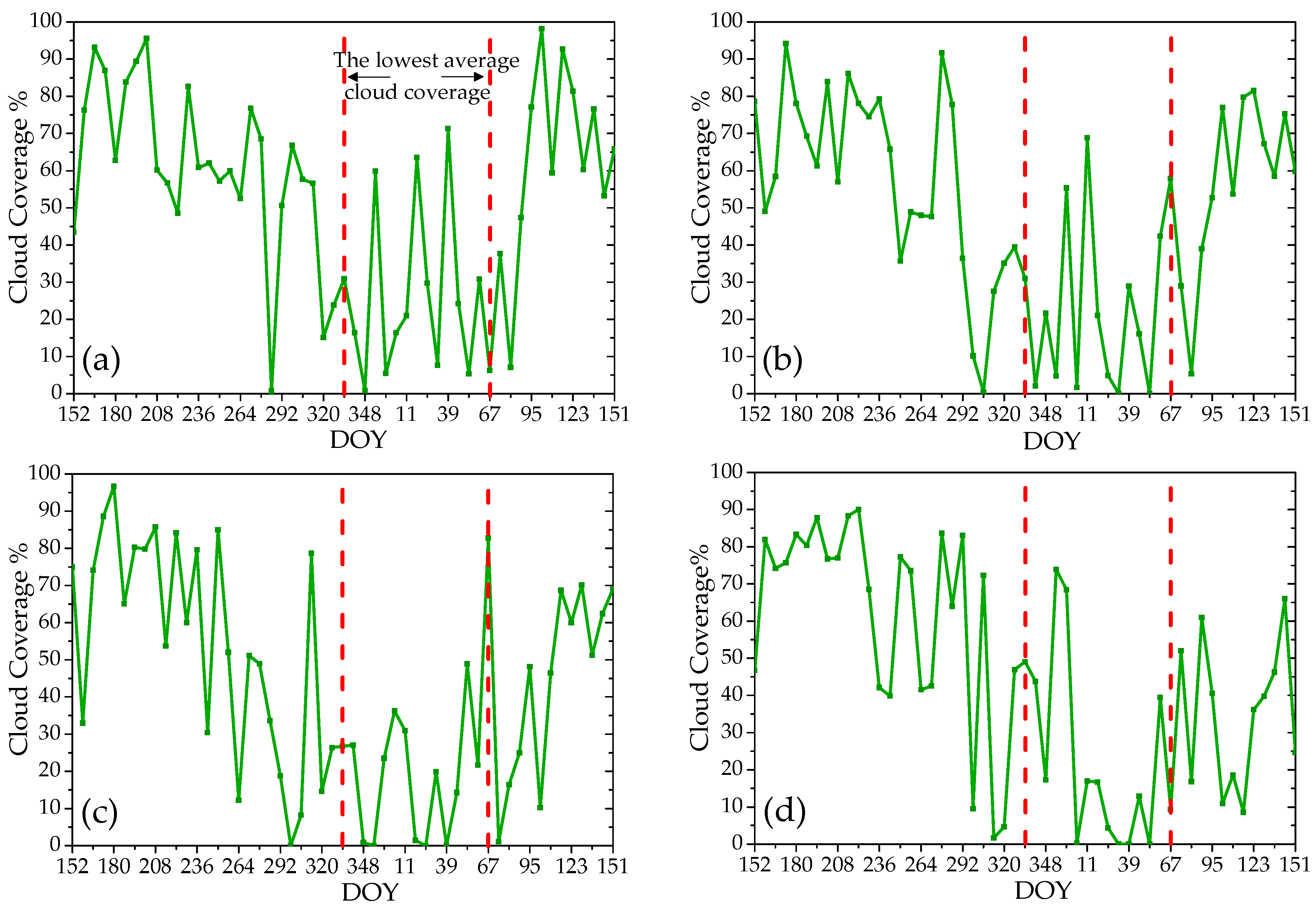
Rubbers are planted in tropical areas where the optical remote sensing images are frequently contaminated by clouds and fog. Xishuangbanna is a tropical monsoon forest climate region where rubber trees shed their leaves in February, and new leaves begin to turn green in late March. To specify the remote sensing window for the extraction of phenological features of rubber trees in this area, the analysis of the cloud coverage frequency is vitally important to the applicability of our method for rubber plantation identification. Therefore, we first used MOD035 data to analyze the average cloud coverage of the study area during four different years: 2000, 2005, 2010, and 2015, which range from June to June of the following year. This period completely covers the entire dry season of Xishuangbanna. There are many more clear days during the dry season than during the wet season. In addition, rubber trees shed their leaves during only this period when many cloud-free optical remote sensing images can be obtained. To improve the representativeness of the daily MOD035 data, we transformed the cloud coverage data to an average of every 7 days. The transformed cloud coverage data were then used to analyze the coverage frequency in Xishuangbanna to specify the proper remote sensing window.
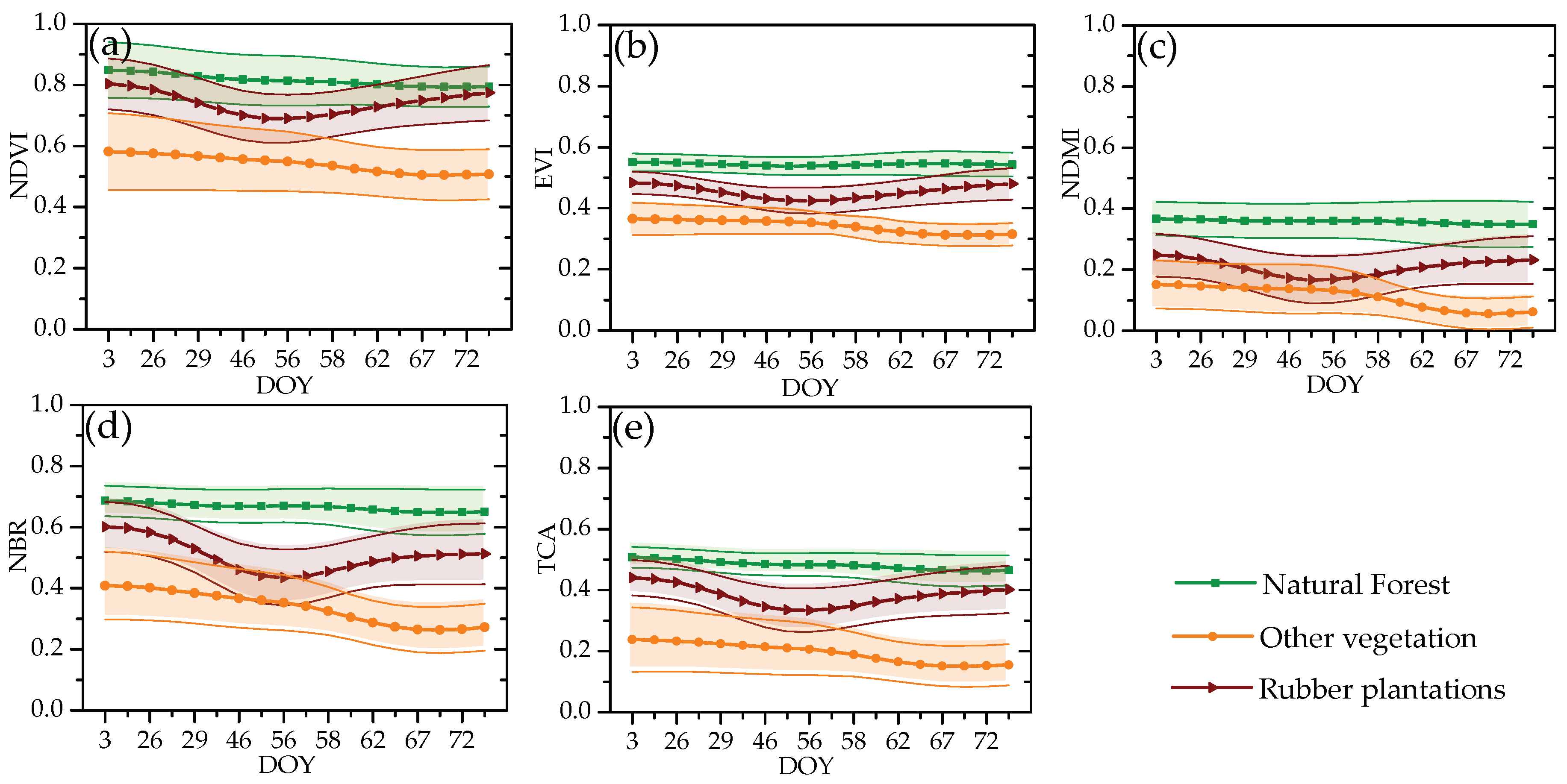
Optical remote sensing images within the chosen remote sensing window were used to derive the changes in phenological features of rubber trees. The phenological features were derived based on the indices calculated from the fused data, including NDVI, EVI, NDMI, NBR, and TCA. Numerous vegetation indices can accurately reflect vegetation growth conditions and capture the trends in vegetation changes. Among these indices, the NDVI is a widely used vegetation index; however, there are some defects, such as its saturation to high vegetation coverage and disturbances caused by atmospheric noise and the soil background [39]. In addition to NDVI, indices such as the EVI, NDMI, NBR, and TCA are commonly used to construct time series data for forest monitoring, and some of these indices have been proven to exhibit better performance over NDVI [40]. This study used these 5 indices to construct the time series data, and the separability of these time series indices was compared and analyzed in rubber plantation classification, and through the fusion of time series data sets, we could obtain accurate annual phenological changes of rubber plantations and the minimum annual vegetation cover of rubber plantation could be obtained, that may be difficult to obtain from a single data (such as, Landsat data) derived phenology, the difference between our method and other methods are summarized in Table 4.
This study finally classified the rubber plantations by applying two machine learning classifiers, the support vector machine (SVM) and random forest (RF), which were trained using the training samples. The SVM classifier is based on statistical machine learning theory to determine the location of decision boundaries that produce an optimal separation of classes. Thus, this nonparametric and sample distribution-free classifier was applied in this study. To estimate the performance of different time series indices, the RF classifier, which is another nonparametric statistical machine learning classifier, was also used. An RF is built based on the predictions from multiple decision trees, where each decision tree is constructed from a different bootstrap sample of the original data set [41]. The features derived from the time series are high-dimensional data sets, and both SVM and RF classifiers are suitable for high-dimensional data classification. Therefore, the RF classifier was selected to be compared with the SVM classifier in this study. In the final step, the accuracies of different classification schemes were assessed based on the validation samples to determine the most suitable approach. The specific process is shown in Figure 2, and the main parts are as follows.

3.1. Analysis of the Optical Remote Sensing Window for Xishuangbanna

This study analyzed the average cloud coverage of the study area from June to June of the following year in four different years: 2000, 2005, 2010, and 2015. Because there are as many as 365 images for each year, remarkable redundancy exists when analyzing the cloud coverage trends during different seasons, so the average cloud coverage was calculated over each 7 day period. The cloud coverage trends for each period are shown in Figure 3. Results indicate that the lowest cloud coverage in the study area (as shown between the two red dotted lines in Figure 3) commonly occurs from December (approximately DOY 327) to early March of the following year (approximately DOY 067). Thus, cloud-free optical remote sensing data are abundant during this period; in contrast, the highest cloud coverage in the study area appears from June to September, and more than 70% of the images are clouded (or fogged). Cloud-free MODIS images mostly occur during the dry season, and there are almost no completely clear images from June to September. Therefore, data between June and September are not suitable for classification of vegetation in Xishuangbanna using optical remote sensing time series data.
According to the field survey, the period from December to March of the following year belongs to the dry season in Xishuangbanna. With the decreases in temperature and precipitation, rubber plantations gradually enter the defoliation period; thus, vegetation indices such as EVI would reach the lowest value in February of the following year. Then, rubber plantations gradually turn green and new leaves began to grow, and the EVI value gradually increases. Therefore, from every November to March of the following year, the vegetation indices of rubber plantations are significantly different from those of other local vegetation. This period is also within the optical remote sensing window of Xishuangbanna, which indicates that the optimum time period for identifying rubber plantations using time series optical remote sensing data is from December to March of the following year.

3.2. Generation of Time Series Indices with High Spatial and Temporal Resolution

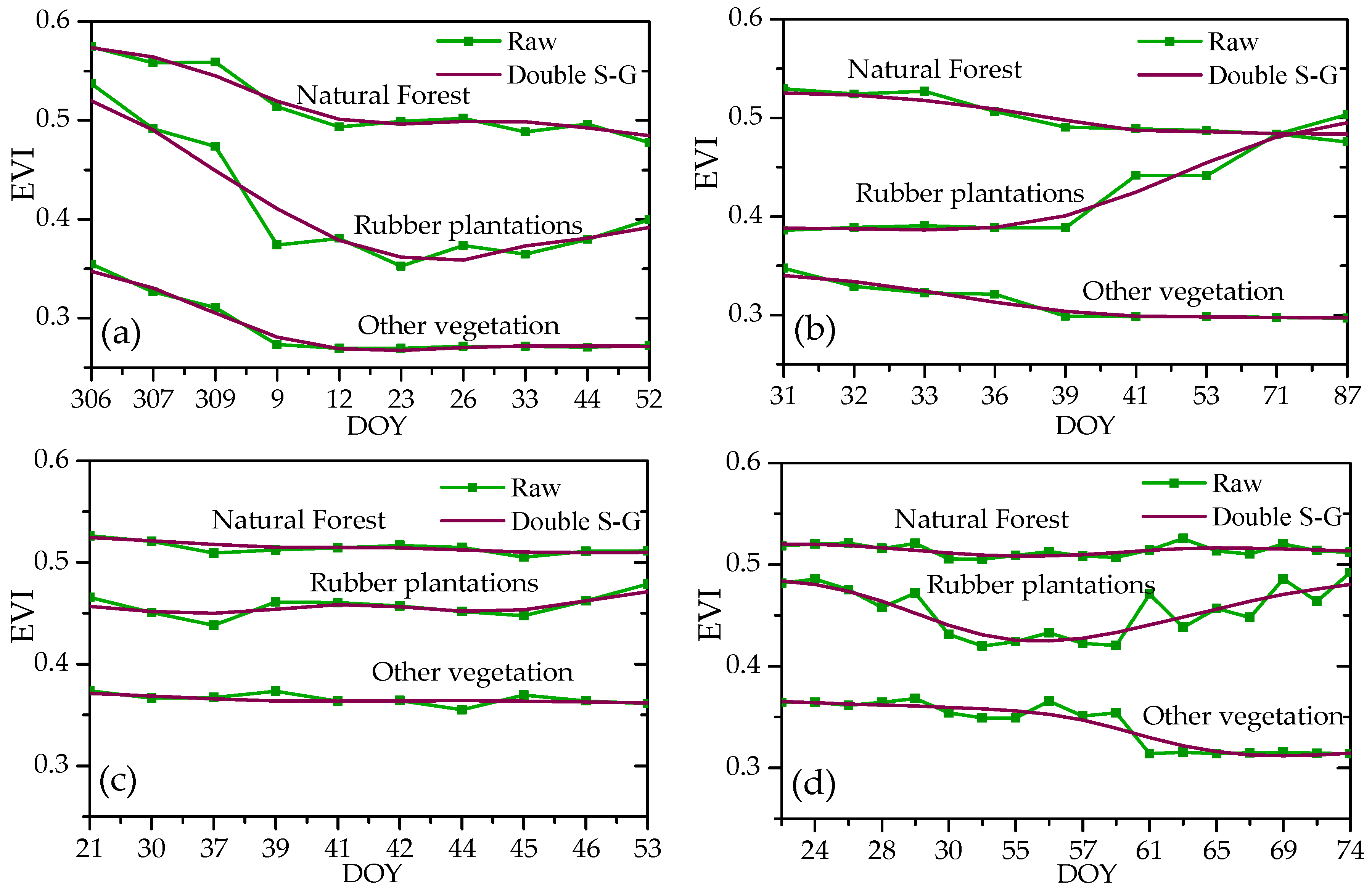
According to the optimum optical remote sensing window in Xishuangbanna, Landsat TM/ETM+/OLI, and MOD09GA data from December to March of the following year were used to fuse and extract the phenological characteristics of rubber plantations and their changes. The ESTARFM requires cloud-free and high-quality remote sensing data as inputs, so cloudless MOD09GA and TM/ETM+/OLI surface reflectance data during the remote sensing window were selected (using the MODIS QC data for MODIS, Fmask for Landsat images) as input data. Five indices were calculated based on the selected cloud-free surface reflectance data for MODIS and Landsat. Then, time series vegetation indices with high spatial and temporal resolution were generated by employing the ESTARFM algorithm. For each of the constructed time series indices, noise inevitably existed because of the directional reflectance of land cover, shadows caused by rugged terrain or atmospheric pollution. These noises are obstacles to time series feature extraction, so we employed a new noise-reduction algorithm based on Savitzky-Golay (S-G) called the Spatial-Temporal Savitzky-Golay (STSG) method to remove the noise, the new method assumes discontinuous clouds in space and employs neighboring pixels to assist in the noise reduction of the target pixel in a particular year [42,43]. This method is a convolution algorithm based on least squares. The main formula is as follows:
Y j = i = m i = m ( C i × Y j ) / N
In Equation (1) ,   Y and Y are vegetation indices before and after filtering; Ci is the least squares fitting coefficient of the high-order polynomial, which is the weight of the i-th EVI value from the filter head; N is the length of the filter, its size is equal to 2m+1, and m is the window radius. The S-G filter can remove most of the noise and smooth the original time series data with good fidelity [44]. Although a single S-G filtering fits well with the basic trend of the original data, noise still exists. Thus, a double S-G filtering (S-G filtering again based on the first S-G filtered results) was performed to remove additional noise, which can also fit the basic trend of the original data well [45].

3.3. Analysis of Data Fusion Accuracy

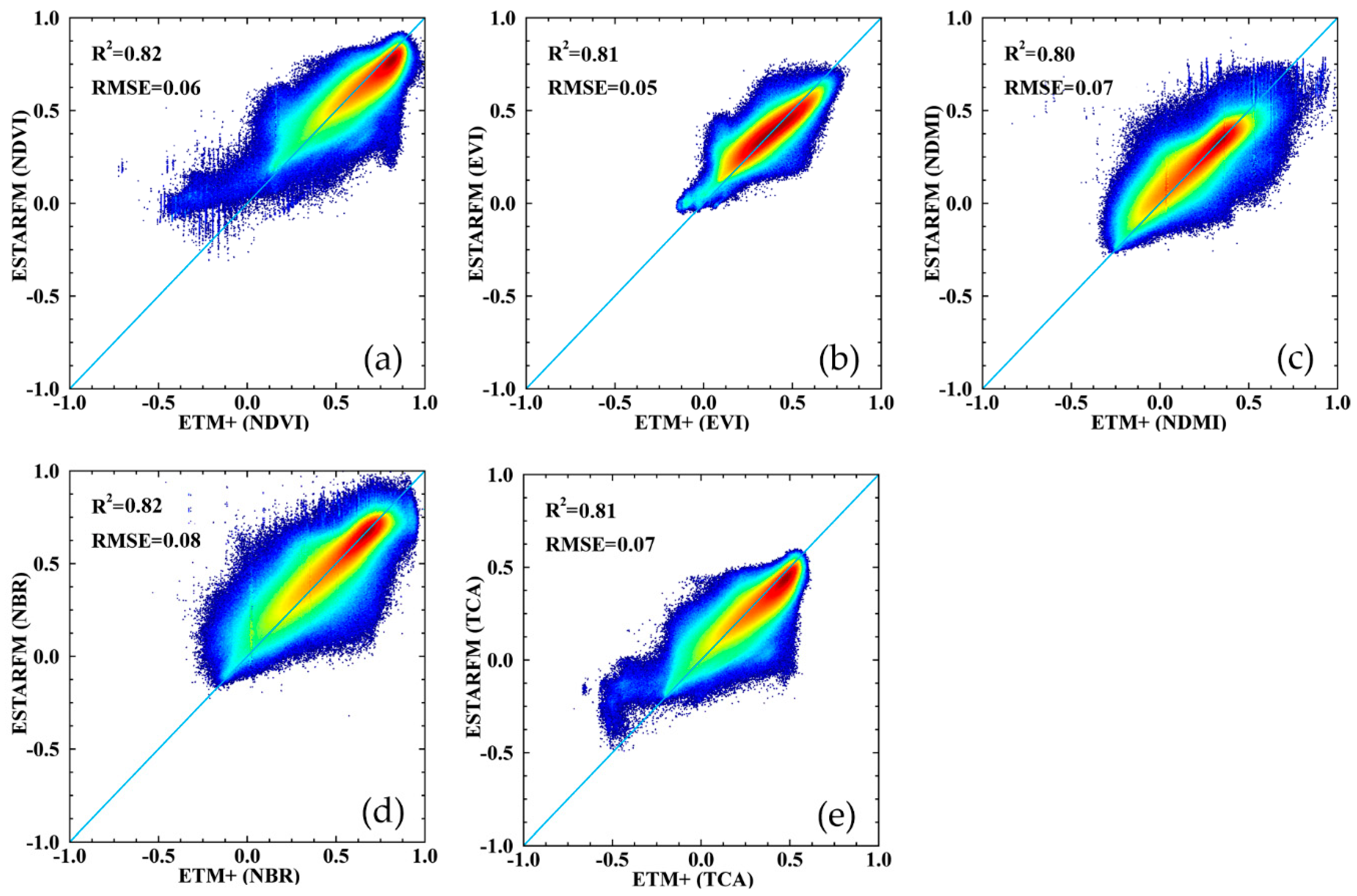
3.3.1. Accuracy Analysis of the 5 Fused Time Series Indices

To assess the data fusion accuracy, it is needed to analyze the correlation between the five indices fused by ESTARFM and the corresponding indices calculated from the observed Landsat data of the same day. For example, to assess the accuracy of the ESTARFM fused indices on DOY 059 of 2015, the input MODIS and Landsat indices were DOY 003 and DOY 067 (time interval of 64 days), respectively. During the accuracy evaluation process, the correlation coefficient (R) between the fused index on DOY 059 and the index derived from the Landsat observation data was calculated. The evaluation index adopts the determination coefficient R2 and root mean square error (RMSE). The closer the determination coefficient R2 is to 1.0, the higher the accuracy of the fusion data is, and the closer it is to 0.0, the lower the accuracy of fused data is. Meanwhile, the closer the RMSE is to 0.0, the higher the accuracy of the fusion data is, and vice versa.

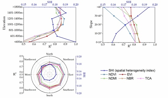
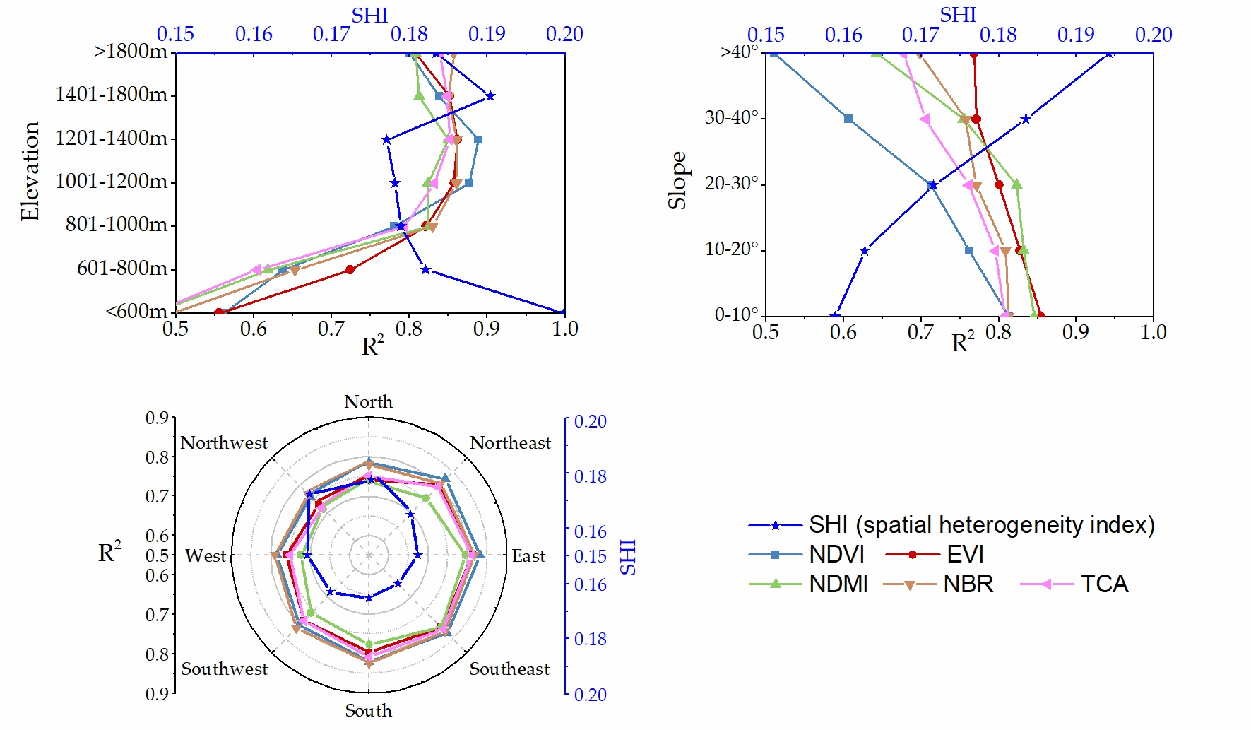
3.3.2. Analysis of Factors Affecting the ESTARFM Fusion Accuracy

In this study, we analyzed the following factors that may affect the ESTARFM fusion accuracy:
(1) The interval of days between input images. Time intervals of 32 days, 56 days, 64 days, and 112 days, this interval was depended on the available observed Landsat data.
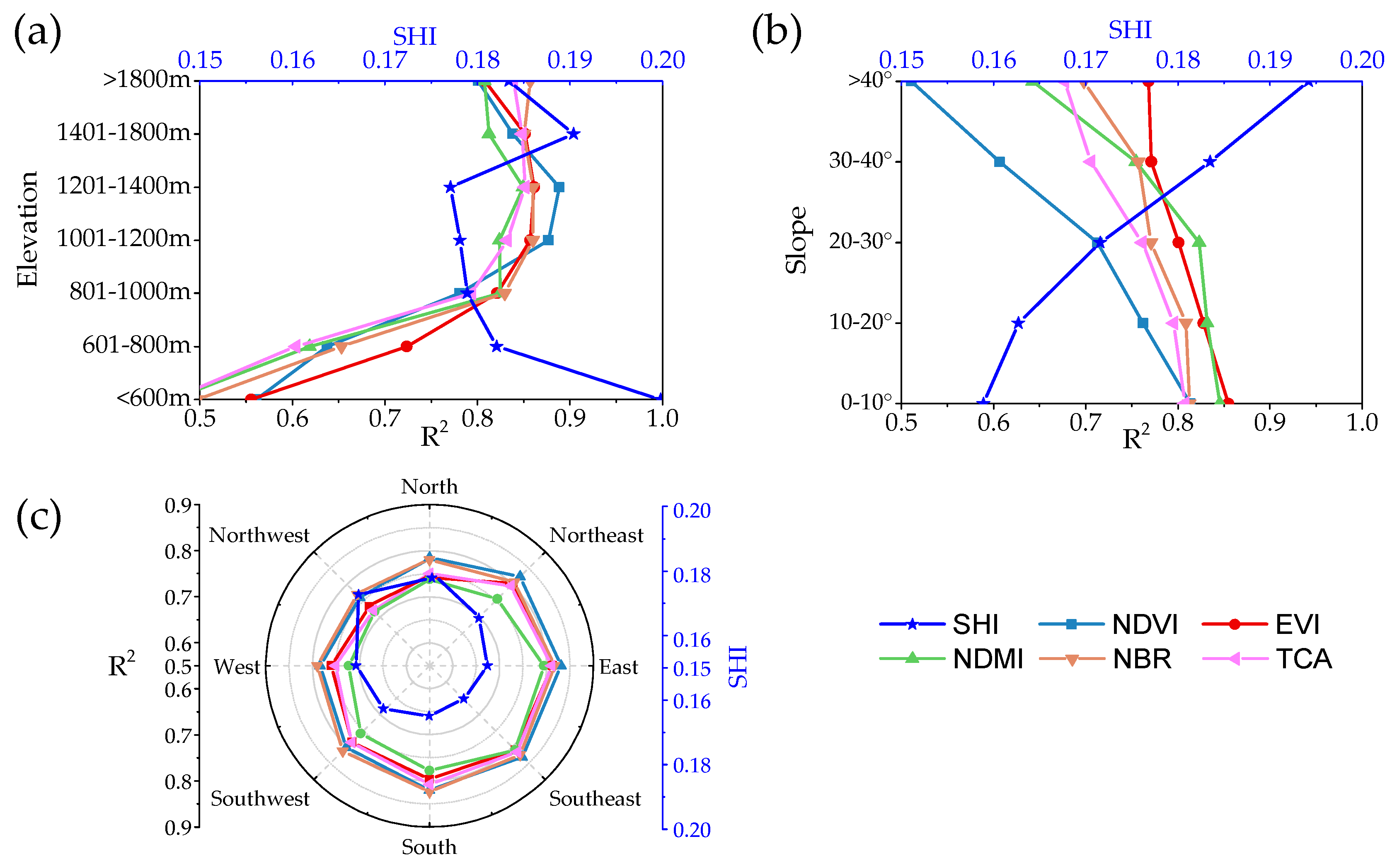
(2) Terrain factors, including elevation, slope, and aspect as following:
(i) Based on DEM data analysis and field investigation, the data fusion accuracy was analyzed by dividing the elevation into seven ranges: less than 600 m.a.s.l., 601–800 m.a.s.l., 801–1000 m.a.s.l., 1001–1200 m.a.s.l., 1201–1400 m.a.s.l., 1401–1800 m.a.s.l., and greater than 1801 m.a.s.l.
(ii) The slopes were divided into 5 grades: 0–10°, 10–20°, 20–30°, 30–40°, and greater than 40°.
(iii) The slope aspect was divided into eight directions; namely, east (67.5–112.5°, semi-shady slope), southeast (112.5–157.5°, semi-sunny slope), south (157.5–202.5°, sunny slope), southwest (202.5–247.5°, sunny slope), west (247.5–292.5°, semi-sunny slope), northwest (292.5–337.5°, semi-shady slope), north (0–22.5°, 337.5–360°, shady slope) and northeast (0–22.5°, 22.5–67.5°, shady slope).
(3) Spatial heterogeneity index. Spatial heterogeneity is one of the main causes of spatial scale effects [46] and may affect the fusion accuracy. To analyze the relationship between spatial heterogeneity and fusion accuracy, we used the spatial heterogeneity index (SHI) proposed by Zhang to quantitatively analyze the relationships between spatial heterogeneity and the three TFs. A SHI of a pixel f ( i , j ) is defined as the sum of the absolute brightness difference between f ( i , j ) and its eight neighboring pixels [47]:
S H I i j = a = 1 1 b = 1 1 | f ( i , j ) f ( i + a , j + b ) |
In Equation (2), S H I i j is the SHI of a pixel f ( i , j ) . The SHI for a region (assuming the image size is m multiplied by n) is defined as:
S H I = 1 m · n i = 1 m j = 1 n S H I i j

3.4. Comparative Analysis of Different Time Series Indices

Vegetation coverage is high in tropical areas, and the response of vegetation change in spectral space is limited and complicated. Therefore, it is necessary to compare and analyze the performance of different time series indices for rubber plantation changes in Xishuangbanna. In this study, 5 time series data sets (such as NDVI, EVI, NDMI, NBR and TCA) were selected for comparative analysis of their separability in rubber plantation classification.

3.4.1. Time Series Index-based Feature Extraction

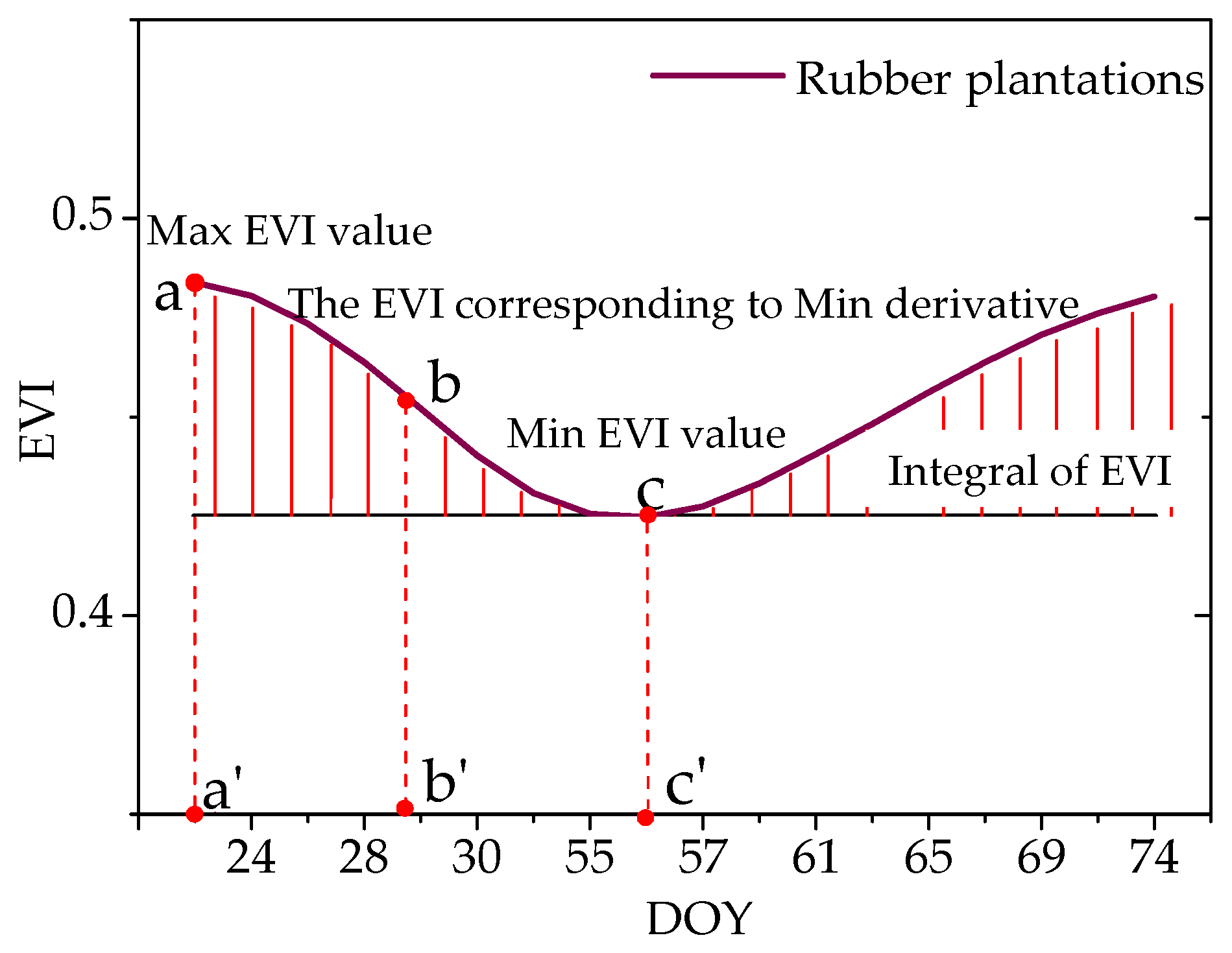
Time series indices fused by the ESTARFM during the key phenophase of rubber plantations contain a large amount of information on the rubber growth state and changes, which are high-dimensional data. Excessive data dimensions may cause data redundancy and reduced classification accuracy. To better extract the time series features based on the fused data sets and remove redundant data, this study extracted six features based on the time series vegetation index curves using IDL (Interactive Data Language). Taking the EVI time series features as an example, as shown in Figure 4, six classification features were extracted in this study, which were the maximum and minimum values of the time series index from December to March of the following year, the integral between the 1st day and the 45th day of the year, the integral of the overall time series index curve, the ratio of the maximum value of the time series index to the integral of the time series index curve, and the date when the minimum derivative of the time series curve could be obtained (detailed in Table 5).
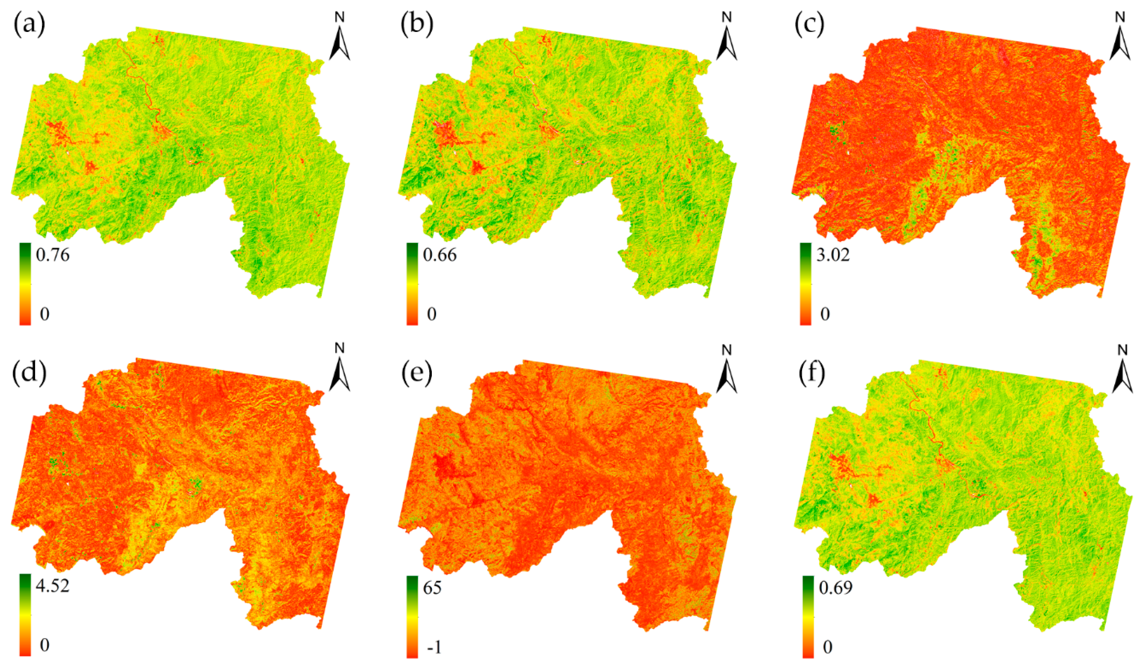
Figure 4 is a schematic diagram showing the time series EVI curve of the rubber plantations within the optical remote sensing window of Xishuangbanna. In this diagram, point a is the maximum EVI value within this remote sensing window, point c is the minimum EVI value, point b is where the minimum EVI derivative value is obtained, indicating the rate of change in deciduous rubber plantations; the time interval from a to c is the deciduous period of rubber plantations, and rubber plantations enter the regreening up period at point c. The integral of EVI corresponds to the biomass within this remote sensing window of Xishuangbanna (selected here from DOY 001 to DOY 045), which are apparently different between different vegetation types. The results of the six features extracted from the study area are shown in Figure 5.

3.4.2. Separability Evaluation of Classification Features

To evaluate the separability of the 6 selected classification features, we need a monotonic criterion that exhibits a monotonic relationship with the classification error rate that can be measured [48]. The most commonly used J-M (Jeffreys-Matusita) distance based on the conditional probability method was used in this study [49]. When a feature follows the normal distribution, the J-M distance can be calculated as [50]:
J M ι j = 2 ( 1 e B ι j )
The B ι j in formula (4) is Bhattacharyya distance [51]:
B i j = 1 8 ( μ ι μ j ) T ( c i + c j 2 ) 1 ( μ ι μ j ) + 1 2 l n ( 1 2 | c i + c j | | c i | | c j | )
In Equation (5), μ ι is the mean of the i-th category and c i is the covariance matrix of the i-th category. The range of J-M distance is [0,2]. J-M distances were calculated according to the selected sample points; a value of greater than 1.38 indicates good separability, values between 1.0 and 1.38 indicate moderately separable, and values less than 1.0 indicate poor separability [52,53]. Taking the EVI time series features of rubber plantations and natural forest as an example, the J-M distances are as follows:
(i) when 2 features were combined, the maximum J-M distance was 1.57, and the corresponding combination was IV and V;
(ii) when 3 features were combined, the maximum J-M distance was 1.80, and the corresponding combination was I, II and V;
(iii) when 4 features were combined, the maximum J-M distance was 1.87 and the corresponding combination was I, II, V and VI;
(ⅳ) when 5 features were combined, the maximum J-M distance was 1.93, and the corresponding combination was I, II, III, V and VI;
(ⅴ) when 6 features were combined, the maximum J-M distance was 1.98.
Then, we analyzed the J-M distances of these six features for NDVI, EVI, NDMI, NBR, and TCA time series indices, as shown in Table 6. The results showed that when the features derived from the EVI time series index were the six features listed in Table 5, the J-M distances of all types (natural forest, rubber plantations, other vegetation, and non-vegetation) were greater than 1.9, which indicates good separability between each of the classes, as shown in Table 6. Therefore, these six features of the EVI time series index can not only remove data redundancy from the original time series curves but also ensure the classification accuracy.

3.5. Classification Schemes

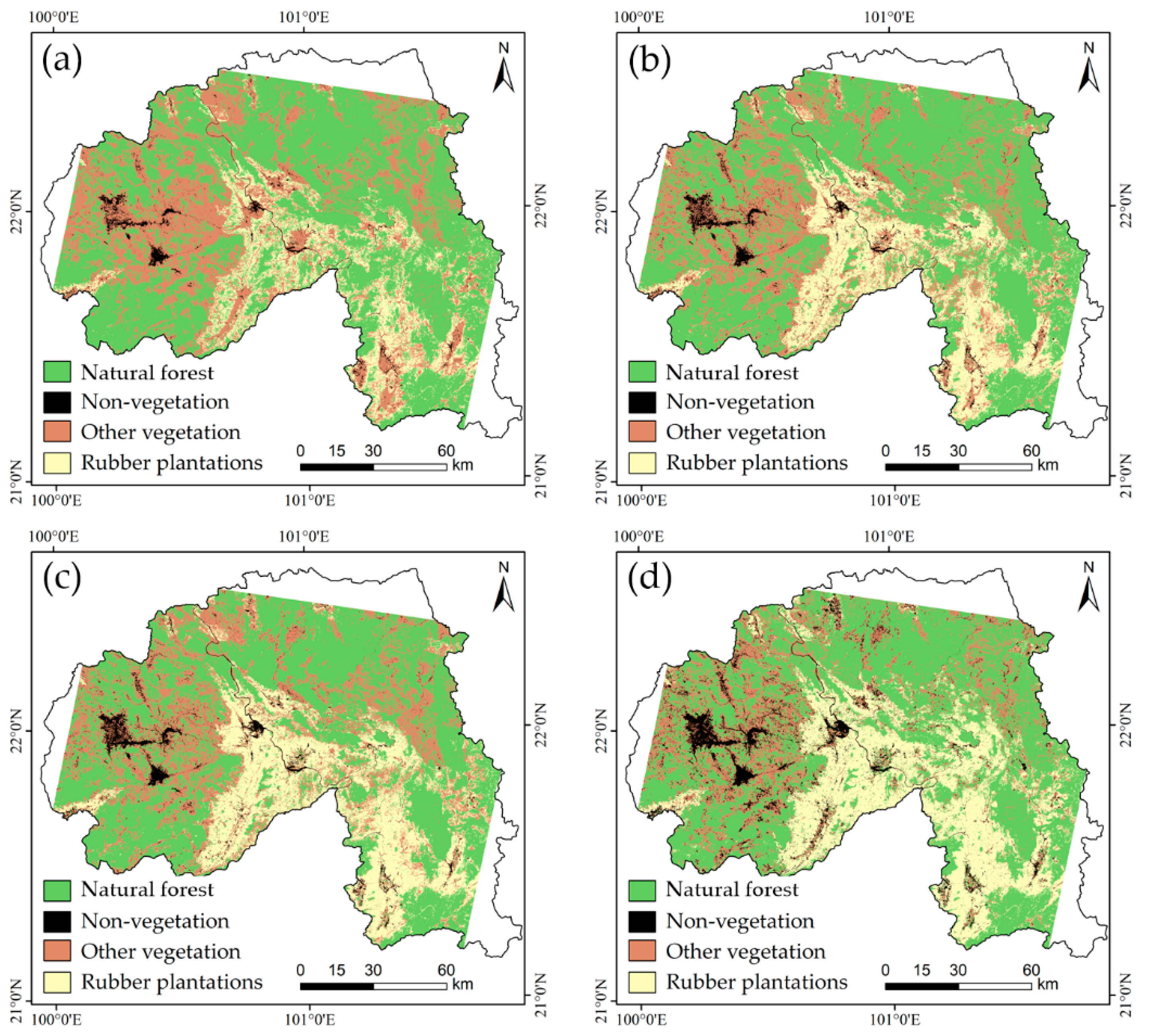
This study analyzed which of the three data sets (monotemporal image, time series data set and selected feature data set) was the best classification data set. The classification schemes we designed are as shown in Table 7. Each of the 3 data sets was classified by employing the SVM and RF classifiers.

4. Results and Discussion

4.1. Data Fusion Accuracy

4.1.1. Accuracy of the 5 Fused Time Series Indices

According to the determination coefficient results of the fused 5 indices in Figure 6, each of the results has an R2 greater than 0.8, which indicates that the fused indices exhibit high correlation with the indices derived from the observed results. The results for 2000, 2005, and 2010 are shown in Table 8. A minimum R2 of 0.66 means R is greater than 0.8 for each of the results, which indicates that the blending method used was feasible to construct time series indices. For all of the fused results, the determination coefficient R2 of NDVI is closer to 1, and its RMSE is closer to 0, so the fused NDVI has the highest correlation with the NDVI calculated from the observed data and the lowest with the NDMI, as shown in Table 8.

4.1.2. Factors Affecting the ESTARFM Fusion Accuracy

The previous analysis showed that there are high correlations between the fused time series indices and the time series indices calculated from the observed data; however, the accuracy of the fused result is affected by other factors: (1) the interval of days between input images. As shown in Table 8, the fusion accuracy decreases when the interval increases from 32 to 112 days. For example, the R2 of the TCA fusion accuracies decrease from 0.81 to 0.67 when the data acquisition interval between input data increases from 32 days to 112 days. (2) Terrain factors. The influences of elevation, slope, and slope aspect on the fusion accuracy were analyzed, and we take the results of DOY 059 in 2015 as an example, as the trend remains the same for the other fusion results.
(i) The fusion accuracy increases with increasing elevation. The results showed that the fusion accuracies were significantly different at different elevations: the fusion accuracy fluctuated greatly between different indices as the elevations changed; the highest fusion accuracy was observed at elevations between 1201 and 1400 m.a.s.l., and the lowest accuracy was observed in areas where the elevation was less than 600 m.a.s.l.
(ii) The fusion accuracy tends to be higher in areas with gentle slopes, but low in areas with steep slopes. The results in Figure 7b show that the fusion accuracy decreases with the increase in slope, and there tends to be a greater negative impact on NDVI in areas with steep slopes. As the slope increases to steeper than 40°, the correlation between the fused NDVI and observed NDVI decreases from 0.82 to 0.52, while the decrease was smaller for EVI, with R2 decreasing from 0.85 to 0.77.
(iii) Slope aspect have less of an influence on the fusion accuracies, but the fusion accuracies were lowest in the northwest. The change in accuracy at the different slope aspects is shown in the wind rose chart in Figure 7c; the circumference represents the slope aspect, and the radius represents the fusion accuracy R2 on each aspect. The R2 from the center of the circle to the top of the radius is from 0.5 to 0.9. The results show that the slope had little influence on the fusion accuracy of the five time series indices, but the fusion accuracy was lowest on the northwest slope (the R2 of the northwest slope was 0.72, approximately 0.08 less than the maximum).
We take the near-infrared (NIR) band of DOY 059 in 2015 to calculate the SHI as an example. The SHIs of different TFs are shown in Figure 7. The results show that the fusion accuracy of the time series index is negatively correlated with spatial heterogeneity: (i) the lowest SHI value occurs at elevations between 1201 and 1400 m.a.s.l., and the highest SHI occurs in areas with elevations less than 600 m.a.s.l.; (ii) the SHI increases with increasing slope, which indicates that rugged terrain tends to have heterogeneous land surfaces; (iii) the SHI is highest on the northwest slope, which means that the coverage on shady slopes tends to be heterogeneous. The results in Table 9 show a considerable negative correlation between the fusion accuracy of the 5 indices and the SHI. The fusion accuracy decreases with the increase in SHI according to Figure 7.

4.2. Choosing Best of the 5 Fused Time Series Indices

Based on the field samples and the time series indices, time series curves are plotted to analyze the separability of natural forests, rubber plantations, and other vegetation cover types; they represent the range of deviations of different indices at the same sample point by calculating the standard deviations, as shown in Figure 8. The time series curves of EVI and TCA for rubber plantations drop obviously around DOY 056 for each of the 5 indices, which indicates that rubber plantations are obviously different from natural forest and other vegetation cover types. The vegetation indices for natural forests are relatively stable because most of the vegetation in Xishuangbanna is evergreen. The curves for the other vegetation cover types exhibit in the lowest values. These results indicate that time series vegetation indices are promising for capturing the different phenological characteristics to identify rubber plantations.
According to the analysis results in the previous section, we used the EVI to analyze the growth characteristics of different vegetation types. Limited by the Landsat acquisition time, the beginning and ending times were different for each of the 4 years. However, the time series vegetation index curves for each of the four years had the same distinguishable features and trends after filtering, as shown by the EVI curves in Figure 9. The features could be summarized as follows. (i) The EVI values from high to low are natural forest, rubber plantations, and other vegetation. (ii) The EVI change trends for rubber plantations are different from those for natural forest and other vegetation types: the EVI values of rubber plantations presented a decreasing trend in January in each year, the lowest value appearing in February of the following year, and the value then began to rise gradually. (iii) There were no strong fluctuations between natural forest and other vegetation types, and the difference between them was remarkable. As Xishuangbanna enters the dry season starting in December when temperature drops and precipitation gradually decreases, rubber plantations enter the defoliation phase, so the EVI value of the rubber plantations shows a decreasing trend in January. Natural forests are dominated by evergreen broad-leaved vegetation, so there was no significant EVI fluctuation during any of the 4 years. The other vegetation types in the study area are dominated by farmland, which is transformed into fallow land from November to April of the following year. During this period, no crops are planted, and the EVI value remained low. Based on the above analysis, the time series indices can capture the difference between rubber plantations and other land cover types as long as key points within the curves can be obtained.

4.3. Accuracy Validation of the Classification Results

4.3.1. Classification Results of Different Classification Schemes Using EVI Time Series Data

This study analyzed three classification schemes in this study. The results are shown in Table 10. (i) The classification accuracy was lowest when a monotemporal image was used, and the overall classification accuracy was 68.49% with a kappa value of 0.54. (ii) The classification accuracy was highest when a selected feature data set was used, which was 3% higher than the accuracy when the EVI time series data set was directly applied. (iii) The classification results of the RF classifier on processed time series and feature data sets are better than those of SVM classifiers (increase of approximately 2%) in this study. These results indicate that selecting features from time series data sets using the RF classifier would be a better choice for classification of time series data.
Figure 10 shows the classification results when using the EVI time series features using the RF classifier with the highest classification accuracy for each of the classification schemes. Table 11 presents the classification accuracy results for 2000, 2005, 2010, and 2015.
The results show that: (i) the planting area of rubber in Xishuangbanna increased rapidly from 221,789 hectares in the year 2000 to 437,686 hectares in 2015. (ii) The rubber planting expansion was mainly between 700 m.a.s.l. and 900 m.a.s.l. from the year 2000 to 2010, and an area of greater than 900 m.a.s.l. between the year 2010 and 2015. (iii) The rubber planting expansion was mainly on slopes that between 15° and 25° from the year 2000 to 2010, and slopes that greater than 25° between the year 2010 and 2015. Rubbers on slops that less than 8° had comparatively less expansion.
The rubber planting area is expanding to high latitude north, and the planting area is expanding from low-altitude valleys to high-altitude mountains. With limited suitable rubber fields in Xishuangbanna, rubber planting is expanding to unsuitable rubber planting areas. The trend of this result is similar to that of study [3].

4.3.2. Classification Accuracies of Different Time Series Indices

The classification results shown in Table 10 indicate that the vegetation index with high spatio-temporal resolution obtained from the fused data can remarkably improve the accuracy of rubber plantation identification, and the classification accuracy of vegetation change features extracted during the key phenological period is higher than that when time series data sets are directly used. To test the performances of different indices, we selected time series features derived from NDVI, EVI, NDMI, NBR, and TCA to conduct the classification using the RF classifier. As shown in Table 12, the classification accuracies of the EVI and TCA time series were higher than those of the NDVI, NDMI and NBR time series, while the classification accuracy of the NDMI time series was the lowest, but the fusion accuracy of EVI obtained by fusion under the same conditions was higher than that of TCA. Therefore, the EVI index should be preferred in future studies.

5. Conclusions

This study presented a rubber plantation identification method based on vegetation phenology in cloudy and foggy tropical areas in this study. The method first analyzed the optical remote sensing window within the study area and then used spatio-temporal data fusion technology to construct a vegetation index data set with high temporal resolution within the remote sensing window. The phenological features of vegetation were captured to map rubber plantations using fused time series indices. The analysis of the presented method and several factors that may affect the high spatio-temporal resolution data fusion accuracy and rubber plantation classification show the following.
(1) Within the optimum optical remote sensing window in Xishuangbanna, fused optical remote sensing data with high spatio-temporal resolution could map the rubber distribution with high accuracy (overall accuracy of 89.51%, kappa of 0.86).
(2) Terrain factors, including the elevation, slope, and aspect, will have obvious negative effects on the accuracy of the fusion of optical data high spatio-temporal resolution: the fusion accuracy of each time series index fluctuated greatly at different elevations; the highest fusion accuracy occurred in areas with elevations from 1201–1400 m.a.s.l., and the lowest accuracy occurred in areas with elevations less than 600 m.a.s.l. The fusion accuracy decreased with the increase in slope, with the least impact on EVI and the greatest impact on NDVI; the slope aspect had less of an influence on the fusion accuracies of the five time series indices, but the fusion accuracy was lowest on the northwest slope. The SHI analysis indicated that land cover heterogeneity increased with decreasing elevation and increasing slope. The land cover types on the northwest slope tend to be heterogeneous compared to those on other slope aspects.
(3) Among the five commonly used time series indices (NDVI, EVI, NDMI, NBR and TCA), the EVI time series had a better ability to capture the different growing features of vegetation in this study. The highest classification accuracies were achieved for the best fusion results of EVI, which indicated that the EVI was the best choice among the five time series indices for time series features-used rubber classification.
The classification method presented in this study was mainly based on the phenological differences between different ground cover types; however, rubber plantations in Xishuangbanna are artificially planted vegetation, which would be affected by human activities to some extent. For example, some rubber trees may still have green leaves during the defoliation phase because of sufficient water and fertilizer conditions. These rubber plantations are more difficult to distinguish using the classification method based on phenological characteristics. The Unmanned Aerial Vehicles’ (UAV) remote sensing is a low-altitude remote sensing platform, which is not disturbed by atmospheric factors in the acquisition of images. It has the advantages that are inaccessible by traditional remote sensing technologies, such as low cost, simple operation, fast acquisition of images and high ground resolution. Therefore, the UAV-based method will become the hot spot of rubber plantations identification and change study in small area in the future. Furthermore, the method proposed by this study is a training samples-based supervised classification method in which the results and accuracies may largely depend on the training sample, which indicates the nonparametric method should be considered in further research. Another deficiency of our method would be the computation complexity, because it needs to fuse images, which is time and computing devices consuming. However, with the development of cloud computing services/devices, this may not be a barrier soon.
Through the fusion of time series data sets, the method can obtain accurate annual phenological changes of vegetation and minimum annual vegetation cover, which is difficult to obtain from a single data source (such as Landsat). This means the method is adaptable and can identify vegetation steadily in different areas. Therefore, this method can be used to identify other vegetation that have distinguishable phenological features in tropical areas. However, the extraction of non-defoliation rubber may perform better if we combine our method with the method proposed by Ye’s study [19], because our method can obtain the rapid and unique growth process of rubber at higher temporal resolution. With the development of remote sensing satellites, higher spatial resolution data with a shorter revisiting period such as Sentinel-2 can be used to study the possible uncertainty in high spatio-temporal resolution data-based classification in future research. For the topographical factors of mountainous tropical areas, directional reflectance and the growth stage of vegetation are strong obstacles to rubber identification accuracy. Thus, it is also necessary to consider the correction of bidirectional reflectance caused by TFs. In addition, the solar zenith angle changes caused by shadows in mountainous areas are also significant influences that should be considered in future research.

Author Contributions

Conceptualization, X.L. and Y.B.; Methodology, X.L. and Y.B.; Data Curation, S.G.; Writing—Original Draft Preparation, S.G.; Formal Analysis, H.Z.; Writing—Review & Editing, X.L., Z.S. and H.Z.

Funding

This work was jointly supported by the National Key Research and Development Program of China (2016YFB0501502), the Applied Basic Research Key Project of Yunnan Province, China (Grant No. 2016FD021), the Water Conservancy Science and Technology Project of Yunnan Provincial Water Resources Department (Grant No. 2014003) and the National Natural Science Foundation of China (Grant No. 41801242). The authors would like to thank the reviewers for their constructive comments for revising this paper.

Acknowledgments

We are thankful to the opening access of the LEDAPS software by NASA, the freely accessible GNSPI and ESTARFM codes by Xiaolin Zhu. The authors would like to thank the reviewers for their constructive comments during the revision of this paper.

Conflicts of Interest

The authors declare no conflict of interest.

Abbreviations

6SSecond Simulation of a Satellite Signal in the Solar Spectrum
ASEANAssociation of South East Asian Nations
AVHRRAdvanced Very High Resolution Radiometer
DEMDigital Elevation Model
DOYDay Of Year
ESTARFMEnhanced Spatial and Temporal Adaptive Reflectance Fusion Model
ETM+Enhanced Thematic Mapper Plus
EVIEnhanced Vegetation Index
GDEMGlobal Digital Elevation Model
GNSPIGeostatistical Neighborhood Similar Pixel Interpolator
HHHorizontal transmitting and Horizontal receiving
HVHorizontal transmitting and Vertical receiving
J-MJeffreys-Matusita
LAILeaf Area Index
LEDAPSLandsat Ecosystem Disturbance Adaptive Processing System
LSWILand Surface Water Index
m.a.s.l.meters above the sea level
MODISMODerate-resolution Imaging Spectroradiometer
MRTMODIS Reprojection Tools
NBRNormalized Burn Ratio
NDMINormalized Difference Moisture Index
NDVINormalized Difference Vegetation Index
OAOverall Accuracy
OLIOperational Land Imager
PAProducer’s Accuracy
UAUser’s Accuracy
Rcorrelation coefficient
RFRandom Forest
SLCScan-Line Corrector
RMSERoot Mean Square Error
SARSynthetic Aperture Radar
S-GSavitzky and Golay
SHISpatial Heterogeneity Index
STARFMSpatial and Temporal Adaptive Reflectance Fusion Model
STSGSpatial-Temporal Savitzky-Golay
SVMSupport Vector Machine
TCATasseled Cap Angle
TFsTerrain Factors
TMThematic Mapper
USGSUnited States Geological Survey
UTMUniversal Transverse Mercator

References

  1. Li, H.; Aide, T.M.; Ma, Y.; Liu, W.; Cao, M. Demand for rubber is causing the loss of high diversity rain forest in SW China. Biodivers. Conserv. 2006, 16, 1731–1745. [Google Scholar] [CrossRef]
  2. Qiu, J. Where the rubber meets the garden. Nature 2009, 457, 246–247. [Google Scholar] [CrossRef] [PubMed] [Green Version]
  3. Chen, H.; Yi, Z.-F.; Schmidt-Vogt, D.; Ahrends, A.; Beckschäfer, P.; Kleinn, C.; Ranjitkar, S.; Xu, J. Pushing the limits: The pattern and dynamics of rubber monoculture expansion in Xishuangbanna, SW China. PLoS ONE 2016, 11, e0150062. [Google Scholar] [CrossRef] [PubMed]
  4. Hainan Provincial Bureau of Statistics. Hainan Statistical Yearbook; China Statistics Press: Beijing China, 2015.
  5. Yunnan Provincial Bureau of Statistics. Yunnan Statistical Yearbook; China Statistics Press: Beijing China, 2015.
  6. Dong, J.W.; Xiao, X.M.; Chen, B.Q.; Torbick, N.; Jin, C.; Zhang, G.L.; Biradar, C. Mapping deciduous rubber plantations through integration of PALSAR and multi-temporal Landsat imagery. Remote Sens. Environ. 2013, 134, 392–402. [Google Scholar] [CrossRef]
  7. Fan, H.; Fu, X.; Zhang, Z.; Wu, Q. Phenology-Based Vegetation Index Differencing for Mapping of Rubber Plantations Using Landsat OLI Data. Remote Sens. 2015, 7, 6041–6058. [Google Scholar] [CrossRef] [Green Version]
  8. Senf, C.; Pflugmacher, D.; van der Linden, S.; Hostert, P. Mapping rubber plantations and natural forests in Xishuangbanna (Southwest China) using multi-spectral Phenological metrics from MODIS time series. Remote Sens. 2015, 5, 2795–2812. [Google Scholar] [CrossRef]
  9. Dong, J.; Xiao, X.; Sheldon, S.; Biradar, C.; Xie, G. Mapping tropical forests and rubber plantations in complex landscapes by integrating PALSAR and MODIS imagery. ISPRS J. Photogramm. 2012, 74, 20–33. [Google Scholar] [CrossRef]
  10. Li, Z.; Fox, J.M. Mapping rubber tree growth in mainland Southeast Asia using time-series MODIS 250 m NDVI and statistical data. Appl. Geogr. 2012, 32, 420–432. [Google Scholar] [CrossRef]
  11. Beckschäfer, P. Obtaining rubber plantation age information from very dense Landsat TM & ETM+ time series data and pixel-based image compositing. Remote Sens. Environ. 2017, 196, 89–100. [Google Scholar] [CrossRef]
  12. Xiao, C.; Li, P.; Feng, Z.; Liu, X. An updated delineation of stand ages of deciduous rubber plantations during 1987-2018 using Landsat-derived bi-temporal thresholds method in an anti-chronological strategy. Int. J. Appl. Earth. Obs. 2019, 76, 40–50. [Google Scholar] [CrossRef]
  13. Xiao, C.; Li, P.; Feng, Z. Monitoring annual dynamics of mature rubber plantations in Xishuangbanna during 1987-2018 using Landsat time series data: A multiple normalization approach. Int. J. Appl. Earth. Obs. 2019, 77, 30–41. [Google Scholar] [CrossRef]
  14. Zhai, D.; Dong, J.; Cadisch, G.; Wang, M.; Kou, W.; Xu, J.; Abbas, S. Comparison of Pixel- and Object-Based Approaches in Phenology-Based Rubber Plantation Mapping in Fragmented Landscapes. Remote Sens. 2017, 10, 44. [Google Scholar] [CrossRef]
  15. Li, P.; Zhang, J.; Feng, Z. Mapping rubber tree plantations using a Landsat-based phenological algorithm in Xishuangbanna, southwest China. Remote Sens. Lett. 2015, 6, 49–58. [Google Scholar] [CrossRef]
  16. Graham, A.; Coops, N.C.; Wilcox, M.; Plowright, A. Evaluation of Ground Surface Models Derived from Unmanned Aerial Systems with Digital Aerial Photogrammetry in a Disturbed Conifer Forest. Remote Sens. 2019, 11, 84. [Google Scholar] [CrossRef]
  17. Anweiler, S.; Piwowarski, D. Multicopter platform prototype for environmental monitoring. J. Clean. Prod. 2017, 155, 204–211. [Google Scholar] [CrossRef]
  18. Chen, B.Q.; Li, X.P.; Xiao, X.M.; Zhao, B.; Dong, J.W.; Kou, W.L.; Qin, Y.W.; Yang, C.; Wu, Z.X.; Sun, R. Mapping tropical forests and deciduous rubber plantations in Hainan Island, China by integrating PALSAR 25-m and multi-temporal Landsat images. Int. J. Appl. Earth. Obs. 2016, 50, 117–130. [Google Scholar] [CrossRef]
  19. Ye, S.; Rogan, J.; Sangermano, F. Monitoring Rubber Plantation Expansion Using Landsat Data Time Series and a Shapelet-Based Approach. ISPRS J. Photogramm. 2018, 136, 134–143. [Google Scholar] [CrossRef]
  20. Chen, B.; Wu, Z.; Wang, J.; Dong, J.; Guan, L.; Chen, J.; Xie, G. Spatio-temporal prediction of leaf area index of rubber plantation using HJ-1A/1B CCD images and recurrent neural network. ISPRS J. Photogramm. 2015, 102, 148–160. [Google Scholar] [CrossRef]
  21. Kou, W.; Xiao, X.; Dong, J.; Gan, S.; Zhai, D.; Zhang, G.; Li, L. Mapping Deciduous Rubber Plantation Areas and Stand Ages with PALSAR and Landsat Images. Remote Sens. 2015, 7, 1048–1073. [Google Scholar] [CrossRef] [Green Version]
  22. Li, Z.; Fox, J.M. Integrating Mahalanobis typicalities with a neural network for rubber distribution mapping. Remote Sens. Lett. 2011, 2, 157–166. [Google Scholar] [CrossRef]
  23. Gao, F.; Anderson, M.C.; Zhang, X.; Yang, Z.; Alfieri, J.G.; Kustas, W.P.; Prueger, J.H. Toward mapping crop progress at field scales through fusion of Landsat and MODIS imagery. Remote Sens. Environ. 2017, 188, 9–25. [Google Scholar] [CrossRef]
  24. Zhao, Y.; Huang, B.; Song, H. A robust adaptive spatial and temporal image fusion model for complex land surface changes. Remote Sens. Environ. 2018, 208, 42–62. [Google Scholar] [CrossRef]
  25. Zhu, X.L.; Liu, D.; Chen, J. A new geostatistical approach for filling gaps in Landsat ETM plus SLC-off images. Remote Sens. Environ. 2012, 124, 49–60. [Google Scholar] [CrossRef]
  26. Wolfe, R.; Masek, J.; Saleous, N.; Hall, F. LEDAPS: Mapping North American disturbance from the Landsat record. In Proceedings of the 2004 IEEE International Geoscience and Remote Sensing Symposium, Anchorage, AK, USA, 20–24 September 2004. [Google Scholar] [CrossRef]
  27. Zhu, Z.; Woodcock, C.E. Object-Based Cloud and Cloud Shadow Detection in Landsat Imagery. Remote Sens. Environ. 2012, 118, 83–94. [Google Scholar] [CrossRef]
  28. Olofsson, P.; Stehman, S.V.; Woodcock, C.E.; Sulla-Menashe, D.; Sibley, A.M.; Newell, J.D.; Herold, M. A global land-cover validation data set, part I: Fundamental design principles. Int. J. Remote Sens. 2012, 33, 5768–5788. [Google Scholar] [CrossRef]
  29. Pengra, B.; Long, J.; Dahal, D.; Stehman, S.V.; Loveland, T.R. A global reference database from very high resolution commercial satellite data and methodology for application to Landsat derived 30m continuous field tree cover data. Remote Sens. Environ. 2015, 165, 234–248. [Google Scholar] [CrossRef]
  30. Zhu, X.L.; Chen, J.; Gao, F.; Chen, X.; Masek, J.G. An enhanced spatial and temporal adaptive reflectance fusion model for complex heterogeneous regions. Remote Sens. Environ. 2010, 114, 2610–2623. [Google Scholar] [CrossRef]
  31. Gao, F.; Masek, J.; Schwaller, M.; Hall, F. On the blending of the Landsat and MODIS surface reflectance: Predicting daily Landsat surface reflectance. IEEE Trans. Geosci. Remote 2006, 44, 2207–2218. [Google Scholar] [CrossRef]
  32. Julia, A.L.; Luis, G.C.; Alonso, L. Multitemporal fusion of Landsat/TM and ENVISAT/MERIS for crop monitoring. Int. J. Appl. Earth. Obs. 2013, 23, 132–141. [Google Scholar] [CrossRef]
  33. Zhu, X.; Helmer, E.H.; Gao, F. A flexible spatio-temporal method for fusing satellite images with different resolutions. Remote Sens. Environ. 2016, 172, 165–177. [Google Scholar] [CrossRef]
  34. Rouse, J.W. Monitoring the Vernal Advancement and Retrogradation (Greenwave Effect) of Natural Vegetation; NASA/GSFC Type III Final Report; NASA/GSFC: Greenbelt, MD, USA, 1974. [Google Scholar]
  35. Liu, H.Q.; Huete, A.R. A feedback based modification of the NDVI to minimize canopy background and atmospheric noise. IEEE Trans. Geosci. Remote 1995, 33, 457–465. [Google Scholar] [CrossRef]
  36. Wilson, E.H.; Sader, S.A. Detection of forest harvest type using multiple dates of Landsat TM imagery. Remote Sens. Environ. 2002, 80, 385–396. [Google Scholar] [CrossRef]
  37. LopezGarcia, M.J.; Caselles, V. Mapping Burns and Natural Reforestation using Thematic Mapper Data. Geocarto Int. 1991, 6, 31–37. [Google Scholar] [CrossRef]
  38. Gómez, C.; White, J.C.; Wulder, M.A. Characterizing the State and Processes of Change in a Dynamic Forest Environment Using Hierarchical Spatio-temporal Segmentation. Remote Sens. Environ. 2011, 115, 1665–1679. [Google Scholar] [CrossRef]
  39. Waring, R.H.; Coops, N.C.; Fan, W. MODIS enhanced vegetation index predicts tree species richness across forested ecoregions in the contiguous USA. Remote Sens. Environ. 2006, 103, 218–226. [Google Scholar] [CrossRef]
  40. Chen, P.Y.; Fedosejevs, G.; Tiscareno-López, M. Assessment of MODIS-EVI, MODIS-NDVI and VEGETATION-NDVI composite data using agricultural measurements: An example at corn fields in western Mexico. Environ. Monit. Assess. 2006, 119, 69–82. [Google Scholar] [CrossRef] [PubMed]
  41. Ahmed, O.S.; Franklin, S.E.; Wulder, M.A.; White, J.C. Characterizing stand-level forest canopy cover and height using Landsat time series, samples of airborne LiDAR, and the Random Forest algorithm. ISPRS J. Photogramm. 2015, 101, 89–101. [Google Scholar] [CrossRef]
  42. Savitzky, A.; Golay, M.J.E. Smoothing and differentiation of data by simplified least squares procedures. Anal. Chem. 1964, 36, 1627–1639. [Google Scholar] [CrossRef]
  43. Ruyin, C.; Yang, C.; Miaogen, S.; Jin, C.; Ji, Z.; Cong, W.; Wei, Y. A simple method to improve the quality of NDVI time-series data by integrating spatiotemporal information with the Savitzky-Golay filter. Remote Sens. Environ. 2018, 217, 244–257. [Google Scholar] [CrossRef]
  44. Chen, J.; Jönsson, P.; Tamura, M.; Gu, Z.; Matsushita, B.; Eklundh, L. A simple method for reconstructing a high-quality NDVI time-series data set based on the Savitzky–Golay filter. Remote Sens. Environ. 2004, 91, 332–344. [Google Scholar] [CrossRef]
  45. Liu, X.L.; Bo, Y.C.; Zhang, J.; He, Y.Q. Classification of C3 and C4 Vegetation Types Using MODIS and ETM plus Blended High Spatio-Temporal Resolution Data. Remote Sens. 2015, 7, 15244–15268. [Google Scholar] [CrossRef]
  46. Steele, J.H. Spatial Heterogeneity and Population Stability. Nature 1974, 248, 83. [Google Scholar] [CrossRef]
  47. Zhang, X.H. Study on Spatial Heterogeneity and Scale Effect of Eucalyptus Forest Based on High Resolution Remote Sensing. Doctoral Dissertation, Nanjing University, Nanjing, China, 2012. [Google Scholar]
  48. Hughes, G. On the mean accuracy of statistical pattern recognizers. IEEE Trans. Inf. Theory. 1968, 14, 55–63. [Google Scholar] [CrossRef]
  49. Bruzzone, L.; Roli, F.; Serpico, S.B. An extension of the Jeffreys-Matusita distance to multiclass cases for feature selection. IEEE Trans. Geosci. Remote 1995, 33, 1318–1321. [Google Scholar] [CrossRef]
  50. Richards, J.A.; Richards, J. Remote Sensing Digital Image Analysis; Springer: Berlin, Germany, 1999. [Google Scholar] [CrossRef]
  51. Kailath, T. The Divergence and Bhattacharyya Distance Measures in Signal Selection. IEEE Trans. Commun. Technol. 1967, 15, 52–60. [Google Scholar] [CrossRef]
  52. Thomas, I.L.; Ching, N.P.; Benning, V.M.; D’Aguanno, J.A. Review Article A review of multi-channel indices of class separability. Int. J. Remote Sens. 2007, 8, 331–350. [Google Scholar] [CrossRef]
  53. Tian, Y.; Chen, H.; Song, Q.; Zheng, K. A Novel Index for Impervious Surface Area Mapping: Development and Validation. Remote Sens. 2018, 10, 1521. [Google Scholar] [CrossRef]
Figure 1. Location of the study area and field survey samples and routes.
Remotesensing 11 00496 g001
Figure 2. Flow chart of this study.
Remotesensing 11 00496 g002
Figure 3. The average cloud coverage was calculated over each 7 day period between June and June of the year: (a) 2000; (b) 2005; (c) 2010; (d) 2015.
Remotesensing 11 00496 g003
Figure 4. Time series EVI curve of rubber plantations and curve features.
Remotesensing 11 00496 g004
Figure 5. Six classification features of rubber plantations based on the EVI time series: (a) max EVI value; (b) min EVI value; (c) integral between DOY 001 and DOY 045; (d) integral of the EVI time series; (e) the ratio of max EVI to the integral of EVI, and (f) the EVI corresponding to the min derivative.
Remotesensing 11 00496 g005
Figure 6. Scatterplots of the predicted data and the observed ETM+ data in 2015: (a) NDVI; (b) EVI; (c) NDMI; (d) NBR; (e) TCA.
Remotesensing 11 00496 g006
Figure 7. Fusion accuracy and SHI of different TFs: (a) Elevation; (b) Slope; (c) Slope aspect.
Remotesensing 11 00496 g007
Figure 8. Time series indices of the 5 indices for land covers in 2015: (a) NDVI time series curve; (b) EVI time series curve; (c) NDMI time series curve; (d) NBR time series curve; (e) TCA time series curve.
Remotesensing 11 00496 g008
Figure 9. The time series of EVI data: (a) time series curves of the main vegetation coverage in 2000; (b) time series curves of the main vegetation coverage in 2005; (c) time series curves of the main vegetation coverage in 2010; (d) time series curves of the main vegetation coverage in 2015.
Remotesensing 11 00496 g009
Figure 10. Classification results for: (a) 2000; (b) 2005; (c) 2010; (d) 2015.
Remotesensing 11 00496 g010
Table 1. The Landsat TM/ETM+/OLI and MODIS data used in this study.
DataMOD03MOD035MOD09GATM/ETM+/OLI
Spatial Resolution1000m1000m500m30m
DOY152(2000)–152(2001)152(2000)–152(2001)306(2000)–052(2001)306(2000)/TM
012(2001)/ETM+
052(2001)/TM
152(2004)–152(2005)152(2004)–152(2005)031(2005)–087(2005)031(2005)/TM
039(2005)/ETM+
087(2005)/ETM+
152(2009)–152(2010)152(2009)–152(2010)021(2010)–053(2010)021(2010)/ETM+
037(2010)/ETM+
045(2010)/TM
053(2010)/ETM+
152(2014)–152(2015)152(2014)–152(2015)003–075(2015)003(2015)/ETM+
059(2015)/OLI
067(2015)/ETM+
075(2015)/OLI
Table 2. Classification system and description.
CategoryDescription
Natural forestNatural forest land and secondary natural forest that are mainly evergreen broad-leaved forests.
Rubber plantationsArtificially planted rubber woodland.
Other vegetationInclude vegetation other than natural forest and rubber (such as farmland, eucalyptus, tea plant, shrubs, etc).
Non-vegetationLand covers such as built-up area and water.
Table 3. Selected Vegetation Indices.
IndexExpressionAuthorRemarks
NDVI N D V I = ρ N I R ρ r e d ρ N I R + ρ r e d Rouse
(1973) [34]
ρ r e d , ρ N I R represent the reflectance at the red and near infrared bands of Landsat images.
EVI E V I = G ( ρ N I R ρ r e d ) ( ρ N I R + C 1 ρ r e d C 2 ρ b l u e + L ) Liu, Huete
(1995) [35]
ρ b l u e ,   ρ r e d ,   ρ N I R are the reflectance at the blue, red and near-infrared bands of Landsat images; G is the gain factor, which was set to 2.5; C1 and C2 are the aerosol impedance coefficients and were set to 6 and 7.5, and L is a background adjustment factor of the canopy, which was 1.0 in this study. In this study, these factors were all set to the most widely used values.
NDMI N D M I = ρ N I R ρ S W I R 1 ρ N I R + ρ S W I R 1 Wilson, Sader
(2002) [36]
ρ N I R , ρ S W I R 1 are the reflectance of the near-infrared and shortwave infrared bands.
NBR N B R = ρ N I R ρ S W I R 2 ρ N I R + ρ S W I R 2 Lopez
(1991) [37]
ρ N I R ,   ρ S W I R 2 represent the ground reflectance values of the near-infrared and shortwave infrared bands, which were originally used to assess the severity of forest fires and later used by scholars to monitor forest changes.
TCA T C A = arctan ( G r B r ) Gómez (2011) [38] B r , G r are the brightness and greenness of the Tasseled Cap transformed results, which are sensitive to the vegetation and soil reflectance.
Table 4. Summary of main rubber plantation extraction methods.
Methods byRemote Sensing DataHigh Spatial/and Temporal Resolution Parametric/
Nonparametric Classification
Study Areas/and Size Obtain Key Phenology Features
Dong et al. [9]MODIS & SARNo/YesParametricHainan, China/LargeYes
Beckschäfer et al. [12]LandsatYes/NoNonparametricXishuangbanna, China/Large No
Ye et al. [20]LandsatYes/NoNonparametricSeima/Small No
Xiao et al. [13]LandsatYes/NoNonparametricXishuangbanna, China/Large No
This studyLandsat & MODISYes/YesParametricXishuangbanna, China/LargeYes
Table 5. Classification features of rubber plantations based on EVI time series.
NumberExtracted FeaturesRangeDescription
ITime series index maximum−1, 1Different types of vegetation time series indices have different maximum values and high discrimination
IITime series index minimum−1, 1Different types of vegetation time series indices have different minimum values and high discrimination
IIITime series exponential curve integration between DOY 001 and DOY 0450, 10In this period, the curve integral expresses the cumulative amount of rubber plantation growth and improves the rubber classification accuracy
IVTime series exponential curve integral0, 39Curve integrals express different growth conditions of different types of vegetation
VThe ratio of time series index maximum to time series exponential curve integral−∞, +∞Using the ratio of different features to improve the distinction of features
VITime series index value corresponding to the time derivative of the time series curve−1, 1The time series index of rubber plantations is different from the maximum and minimum values, which is better distinguished from other vegetation types
Table 6. The maximum J-M distance between classes when 6 features are selected.
ClassesJ-M
NDVIEVINDMINBRTCA
Rubber plantations v.s. Natural forest1.961.981.981.981.97
Rubber plantations v.s. Other vegetation1.921.931.851.911.93
Rubber plantations v.s. Non-vegetation1.991.991.931.931.99
Natural forest v.s. Other vegetation1.941.991.981.991.99
Natural forest v.s. Non-vegetation1.981.991.921.971.99
Other vegetation v.s. Non-vegetation1.891.961.901.881.94
Note: The gray background indicates the maximum value of the corresponding classification feature.
Table 7. Summary of classification schemes.
SchemeDescription
Monotemporal imageUsing a single index within evergreen broad-leaved natural forests in February
Time series data setThe fused time series data set without feature selection or dimension reduction
Selected feature data setThe 6 selected classification features from the fused time series data set
Table 8. Correlation between fused indices and those derived from observed data for different years.
2000200520102015
IndexR2RMSER2RMSER2RMSER2RMSE
NDVI0.760.070.910.050.890.060.820.06
EVI0.700.080.910.030.840.050.810.05
NDMI0.660.090.850.050.810.070.800.07
NBR0.690.090.890.070.820.070.820.08
TCA0.670.090.870.060.820.070.810.07
Interval of 112 daysInterval of 32 daysInterval of 56 daysInterval of 64 days
Table 9. Correlation between fusion accuracy and SHI.
IndexNDVIEVINDMINBRTCA
R
TF
Elevation−0.68−0.78−0.75−0.73−0.67
Slope−0.99−0.95−0.95−0.97−0.99
Slope aspect−0.63−0.62−0.63−0.73−0.68
Table 10. Classification accuracies comparison of different classification schemes.
SchemeOverall Accuracy/%Classifier
2000200520102015
Monotemporal image72.4872.4870.6872.59SVM
69.7574.7968.4970.39RF
Time series data set 80.4381.4280.2582.75SVM
84.8082.5583.1984.26RF
Selected feature data set85.6586.5987.7287.41SVM
87.2086.9188.8589.51RF
Note: The gray background indicates the highest classification accuracy of the corresponding year.
Table 11. Classification accuracies in 2000, 2005, 2010, and 2015.
YearRubber PlantationsNatural ForestOther VegetationNon-VegetationTotal
PA/%UA/%PA/%UA/%PA/%UA/%PA/%UA/%OA/%Kappa
200078.0689.1394.5191.6880.8383.6288.0097.5087.200.82
200584.6593.9697.3297.3279.1470.7570.5370.8186.910.81
201093.0795.4397.7790.5073.3882.9375.9371.9388.850.84
201584.6896.9192.5491.8589.3371.2890.8396.1289.510.86
Table 12. Classification accuracies of different time series index classification methods.
IndexOverall Accuracy/%
Year EVITCANDVINBRNDMI
200087.2086.3984.8080.8675.53
200586.9187.4282.5081.4274.79
201088.8587.7284.1683.1978.67
201589.5188.5785.7881.9577.15
Note: The gray background indicates the maximum value of the corresponding year.

