Abstract
In order to reconstruct a high spatial and high spectral resolution image (H2SI), one of the most common methods is to fuse a hyperspectral image (HSI) with a corresponding multispectral image (MSI). To effectively obtain both the spectral correlation of bands in HSI and the spatial correlation of pixels in MSI, this paper proposes an adversarial selection fusion (ASF) method for the HSI–MSI fusion problem. Firstly, the unmixing based fusion (UF) method is adopted to dig out the spatial correlation in MSI. Then, to acquire the spectral correlation in HSI, a band reconstruction-based fusion (BRF) method is proposed, regarding H2SI as the product of the optimized band image dictionary and reconstruction coefficients. Finally, spectral spatial quality (SSQ) index is designed to guide the adversarial selection process of UF and BRF. Experimental results on four real-world images demonstrate that the proposed strategy achieves smaller errors and better reconstruction results than other comparison methods.
1. Introduction
In remote sensing, optical spectral image plays an important role. Due to the limits of the imaging platform, acquisition devices are usually designed with a tradeoff between spatial and spectral information [1]. Therefore, the remote sensing platform can capture hyperspectral images (HSI) with low spatial high spectral resolutions, multispectral images (MSI) with high spatial low spectral resolutions, and high spatial resolution panchromatic images (PAN), repsectively. Since HSI has hundreds of continuous narrow spectral bands from visible to near-infrared wavelength, it is widely used to describe spectrum divergences of different materials [2]. In many applications, how to obtain a high spatial and high spectral resolution image (H2SI) has received more and more attention. Considering that MSI with higher spatial but lower spectral resolutions compared to HSI, fusing MSI and HSI is an attractive method to generate H2SI.
In recent years, various methods have been proposed for HSI–MSI fusion problems, which can be roughly divided into pan-sharpening based methods and spectral unmixing based methods. The original pan-sharpening algorithm was proposed to fuse MSI with the corresponding PAN [3,4,5,6,7], which can be regarded as a special case of the HSI–MSI fusion problem [8]. Therefore, there are numerous studies to generalize existing pan-sharpening methods for HSI–MSI fusion. These pan-sharpening based HSI–MSI fusion methods usually map the spectral information of HSI to MSI. With the guidance of HSI, the spectral information of each pixel in MSI is enhanced. The first attempt of pan-sharpening based fusion method for HSI and MSI was proposed in [9,10,11] using a wavelet technique, which completed the fusion work in the transform domain. Considering the different characteristics of bands, Chen et al. proposed a framework that solved the HSI–MSI fusion problem by dividing the spectrum of HSI into several regions and fusing band images in each region using conventional pan-sharpening algorithms [12]. Sparse representation (SR) was widely used for image fusion in recent years, which was beneficial to preserve the texture information of different images as [13]. Inspired by SR, a recent SR based pan-sharpening method was applied to HSI–MSI fusion in [14,15], and the authors proposed the spectral grouping concept to split the computationally expensive problem of sharpening the entire HSI into multiple pan-sharpening problems. In order to make full use of the tiny information contained in MSI, Selva et al. proposed a framework called hyper-sharpening that synthesizes a high-resolution image for each HSI band as a linear combination of MSI band images via linear regression [16]. Pan-sharpening based HSI–MSI fusion methods usually make full use of the spatial structural characteristics of MSI. However, the fusion results usually contain spectral distortions due to no consideration of the spectral correlation of bands.
Meanwhile, the spectral unmixing based HSI–MSI fusion techniques have been greatly developed. Spectral unmixing is usually adopted to analyze the composition of mixed pixels, which splits mixed pixels into endmembers and corresponding abundance. Regarding the ideal H2SI as the product of endmember matrix and abundance matrix, the HSI–MSI fusion problem can be converted to an unmixing problem. In order to solve the ill-posed optimization problem, non-negative matrix factorization (NMF) was adopted in reference [17] to obtain the endmember matrix by unmixing of HSI, and the abundance matrix from MSI was obtained by least squares regression. To improve the accuracy of abundance information, Yokoya et al. proposed coupled NMF (CNMF), which estimated the endmember and abundance matrices via alternating spectral unmixing towards HSI and MSI [18,19]. Based on the spectral sparsity, Akhtar et al. [20]. obtained the endmember by sparse dictionary learning, and acquired abundance matrix by sparse coding, respectively. Recently, the sparse regularization widely used in spectral unmixing research was introduced into the HSI–MSI fusion problem [21,22], assuming that the number of endmembers at each pixel is small compared to the number in the endmember matrix. Another abundance regularization called vector-total-variation was proposed by Simões et al. [23], which controlled the spatial distribution of subspace coefficients, where the subspace can be defined either by singular value decomposition (SVD) or by endmember spectral signatures. In [24], Chen et al. proposed an interactive feedback scheme for spatial resolution enhancement, in which spectral unmixing was used as a prior for spatial resolution enhancement. Spectral unmixing based methods split the H2SI into an endmember matrix and an abundance matrix. Each column in the abundance matrix can be regarded as the reconstruction coefficient of a certain pixel in MSI, thus the abundance matrix can effectively preserve the spatial correlation of pixels in MSI. However, the endmember matrix is only a set of basis vectors of the HSI, and there is no way to preserve the spectral correlation of bands in HSI, which could degrade the final fusion results.
To ensure that the final H2SI keeps both the spatial correlation in MSI and the spectral correlation in HSI, we propose the adversarial selection fusion (ASF) method. Firstly, the conventional unmixing based fusion (UF) method is adopted to obtain a preliminary H2SI, which focuses on keeping the spatial correlation of pixels in MSI. Then, to acquire the spectral correlation of bands in HSI, the band reconstruction-based fusion (BRF) method is proposed, which reconstructs another preliminary H2SI by the optimized band image dictionary and reconstruction coefficients. Finally, Spectral-Spatial Quality (SSQ) index is designed to evaluate the two preliminary fusion data, and the final H2SI is generated in the adversarial selection process with SSQ index as guidance. Our contributions mainly include: Propose the BRF method, define the SSQ index to evaluate the quality of the preliminary fusion results, and propose the adversarial selection strategy to combine UF and BRF for better fusion results.
The remainder of this paper is organized as follows. Section 2 introduces the methodology of the adversarial selection fusion (ASF) model, including the sensor observation model, UF method, the proposed BRF method, and the adversarial selection strategy. To demonstrate the effectiveness of our proposed method, Section 3 presents the experimental results on four data sets. Finally, the conclusion is shown in Section 4.
2. Methodology
Figure 1 shows the adversarial selection fusion (ASF) model mainly consisted of three parts, including the unmixing based fusion (UF), band reconstruction-based fusion (BRF), and SSQ based adversarial selection. In UF, a preliminary fusion result was obtained by the product of the endmember matrix and high spatial resolution abundance matrix. As the UF method only considers the spatial correlation in MSI, the BRF method is proposed to acquire the spectral correlation in HSI. In BRF, another preliminary fusion result was reconstructed by the product of band image dictionary and reconstruction coefficients. Finally, Spectral-Spatial Quality (SSQ) indexes of the two preliminary fusion data were calculated, and the final H2SI was generated in the adversarial selection process with the SSQ indexes as guidance.
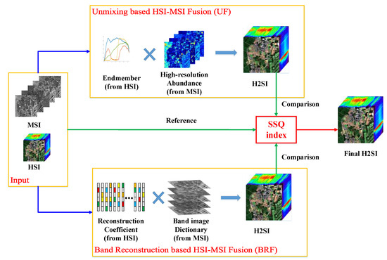
Figure 1.
Illustration of the adversarial selection fusion (ASF) model for hyperspectral image (HSI) and multispectral image (MSI).
Furthermore, the sensor observation model was firstly introduced for better understanding of the mathematical relationship of HSI and MSI. Then, the UF method and BRF method were described in detail, and the SSQ based adversarial selection strategy was showed at the end.
2.1. Sensor Observation Model
Both HSI and MSI are 3D arrays or tensors, which are often called image cubes. For better formulation, these image cubes were denoted in 2D matrix form as, with each column representing the spectral response of a pixel. Here, is the number of pixels, and is the number of bands. In this paper, represented HSI, MSI, and the target H2SI, respectively. and mean the pixel number of down-sampled HSI and band number of down-sampled MSI, respectively. As the definitions show, H2SI had the same band number as HSI, and the same pixel number as MSI. As reported in reference [19], HSI was the spatial degraded form of H2SI, while MSI was its spectral degraded form.
With these representations, the hyperspectral measurement was modeled [1] as follow:
where represents the transform of the point spread function (PSF) from the H2SI () to HSI (), which describes the spatial response of the hyperspectral sensor. More specifically, spatial simulation was performed using an isotropic Gaussian PSF with a full width at half maximum (FWHM) of the Gaussian function. represents the model residual such as the optical and electronic noises, which are identically distributed across the bands and pixels.
Similarly, the multispectral measurement was modeled as:
where is the spectral response transform matrix, with each row representing the transform of spectral response function from to. is similar to , meaning the model residual.
When applied to real data, was determined by the estimation of the PSF. The spectral response function was derived by radiometric calibration. Therefore, and were assumed to be known in this paper. In the experiments, we treated the original hyperspectral data as the reference fusion result, and firstly generated the MSI by Equation (2) and the low spatial resolution HSI by Equation (1).
2.2. Unmixing Based HSI–MSI Fusion
UF methods have achieved good results in preserving the spatial structural information by obtaining more accurate endmember and abundance information. Therefore, in this paper, the UF method was adopted to dig out the spatial correlation in MSI. Spectral unmixing aims at finding out the composition of the mixed pixels by obtaining endmember spectral information and abundance information [25] (the proportion of the various pure materials in mixed pixels). In other words, all spectral images could be represented as the product of the endmember matrix and abundance matrix, which can perfectly build the mathematical relationship between HSI, MSI, and H2SI in the fusion problem. According to the commonly used linear mixture model, the H2SI can be described as follows:
where is the endmember matrix, with each column representing the spectrum of a certain endmember, and is the number of endmembers. is the abundance matrix, with each column denoting the abundance values of all endmembers at the th pixel. It is worth noting that all values in these matrices are non-negative due to their physical meaning.
Therefore, as for HSI–MSI fusion problem, by substituting Equation (3) into Equations (1) and (2), and can be approximated as:
where, and are the spatially degraded abundance matrix and the spectrally degraded endmember matrix, respectively. Thus far, as Figure 2 shows, the HSI–MSI fusion problem converts to dig out the optimal endmember matrix and abundance matrix from HSI and MSI. However, compared to the convolutional unmixing problem, there are two degraded images as inputs instead of a single spectral image. Using the spectral unmixing algorithm directly on HSI to extract the endmember information usually results in inaccurate endmember spectra, thus it is necessary to make full use of the close mathematical relationship between HSI and MSI. In other words, is the spatial degraded form of , and is the spectral degraded form of.
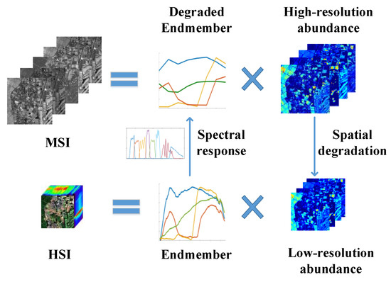
Figure 2.
Illustration of unmixing-based fusion (UF) strategy.
Therefore, in order to obtain the fusion result, we need to search the optimized forms of and to satisfy Equations (4) and (5). Then, the HSI–MSI fusion problem is converted to the following optimization problem [23,26]
In the Equation (6), ‖· denotes the Frobenius norm, which aims at minimizing the residual errors in the linear spectral mixture models. The first term means the estimated fusion data should be able to express HSI, while the second term corresponds to MSI. The parameter controls the relative importance of the various terms.
In this paper, we select the CNMF method to perform the process of UF, which alternately unmixes and by NMF to estimate and. Specifically, we first initialized by vertex component analysis (VCA). Then, repeated NMF on to optimize and and performed NMF on to optimize and until convergence. The endmember matrix and abundance matrix are non-negative, and the sum of the abundances for each pixel can be assumed to be at unity, which is called abundance sum-to-one constraint (ASC). To satisfy the ASC, we used the method given in reference [27], which was implemented by adding a uniform vector into the last row of and (also and ) during the calculation process.
2.3. Band Reconstruction-Based HSI–MSI Fusion
The UF method can obtain the spatial correlation in MSI, but the spectral correlation contained in HSI is ignored. In order to take both the spatial and spectral correlation into account, the BRF method was proposed in this section. Regarding the ideal H2SI as the product of band image dictionary and reconstruction coefficients, BRF acquires the spectral correlation in HSI by optimizing the reconstruction coefficients. The details of the BRF method are as follows.
With high-density spectral bands, the high spectral resolution images are inevitably highly correlative in spectral dimension [28]. In other words, high spectral resolution images are sparse in spectral dimension [29,30], which makes it possible to search a fine band image dictionary used to reconstruct all band data. Here, the band-image dictionary means each element in this dictionary is constituted by pixel values from a single band. It is necessary to emphasize that all values in this dictionary are obtained by solving optimization problems instead of directly assigning by certain methods. The idea of band reconstruction was also used in other HSI researches such as super-resolution reconstruction, band selection, and classification [31], achieving some effective results. Here, we proposed the BRF technique to perform HSI–MSI fusion.
Firstly, H2SI can be represented as the product of a band image dictionary and reconstruction coefficient matrix as follow:
where represents the H2SI, and each row is a vectorial representation of a band. was the band image dictionary, with each row representing the shared band image, and being the number of elements in the dictionary. was the reconstruction coefficient matrix, with each row representing the linear reconstruction coefficients for . Thus, the HSI–MSI fusion problem was converted to search the optimal band image dictionary and reconstruction the coefficient matrix. In this process, we obtain the reconstruction coefficient information from HSI, which effectively provides the spectral correlation of the bands.
Based on band reconstruction, we substituted Equation (7) into Equations (1) and (2), thus and can be presented in the following forms:
same as the definition of and in the UF method, was the spatial degraded version of, while was the down-sampled version of . Figure 3 showed the relationship of these two formulas, and the final fusion data will be obtained by the product of and.
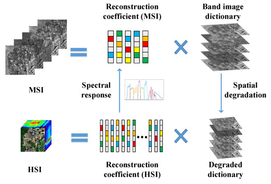
Figure 3.
Illustration of band reconstruction-based fusion (BRF) strategy.
For optimizing and , we define:
We adopted multiplicative update rules to alternately optimize these two items in Equation (10), which were guaranteed to converge to local optima under the non-negativity constraints of two factorized matrices [32,33]. The updated rules were given as:
where denotes the transposition of the matrix, and denotes element wise multiplication and division, respectively. More specifically, the optimization algorithm for the BRF method was summarized in Algorithm 1.
As the algorithm summarizes, we firstly used to initialize because it was simple and beneficial to convergence. The dictionary elements’ number in the dictionary was simultaneously denoted as the band number of MSI, especially , which can be assigned too. Then we optimized and alternately until meeting the termination conditions. In step 2, we applied NMF on Equation (10) to optimize. As the initialization phase, was obtained by. was updated by Equation (11) until convergence, with fixed. As the optimization phase, both and were alternately updated by Equations (11) and (12) until the next convergence.
In step 3, similar procedures were adopted to optimize. As the initialization phase, was obtained by. This process was important in inheriting the reliable reconstruction coefficient information obtained from HSI. Then we updated by Equation (14) until convergence, with was fixed the optimization phase, and were alternately updated by Equations (13) and (14) until the next convergence.
| Algorithm 1 Band Reconstruction-based HSI–MSI Fusion (BRF) algorithm. |
| Input: Low spatial high spectral resolution HSI , high spatial low spectral resolution MSI, spatial response function, and spectral response function. |
| Output: Band image dictionary and reconstruction coefficient matrix. |
| Step 1. |
| Initialization.Initialize as, (the number of rows in) is assigned as the band number of . |
| Step 2. NMF of . |
| (2a) Initialize by , and update by (11) until convergence, with fixed. |
| (2b) Optimize and by (11) and (12) alternately. |
| Step 3. NMF of . |
| (3a) Initialize by , and update by (14) until convergence, with fixed. |
| (3b) Optimize and by (13) and (14) alternately. |
| Step 4. Repeat Steps 2 and 3. |
Step 2 and 3 were repeated alternately until convergence. By alternately updating and, this procedure took advantage of the spectral information of HSI and the spatial information of MSI. Finally, we could reconstruct the H2SI by the product of and as in Equation (7). In other words, we got the final result by reconstructing each band image using the band image dictionary and corresponding coefficients. In the experiments, we first equally divided the input (HSI and MSI) into multiple regions, and then performed BRF in each region independently, which was more efficient and beneficial to find the optimized band image dictionary.
Compared with the UF method, which takes the sparsity of spatial dimension into account, BRF considers the sparsity in spectral dimension. In addition, different initialization means are adopted in the optimization of UF and BRF. In UF, we initialized the endmember matrix using the endmember spectra extracted from HSI. In BRF, we initialize the band image dictionary as bands in MSI. Different initialization methods will greatly affect the final results, which means that UF and BRF methods can acquire very different fusion results. UF regards the fusion data as the product of the endmember matrix and abundance matrix, and reconstructs the fusion data pixel by pixel. In this process, the abundance matrix preserves the spatial correlation of pixels in MSI. As for the BRF method, the reconstruction coefficient information obtained from HSI can acquire its full spectral correlation of bands. That is to say, these two methods solve the HSI–MSI fusion problem from two different but complementary aspects, resulting in two complementary fusion results. For better fusion performance in both spatial and spectral dimensions, in this paper, the SSQ index is proposed to effectively synthesize these two aspects, which will be introduced in detail in the next section.
2.4. Spectral-Spatial Quality Index based Adversarial Selection Strategy
In order to combine the advantages of UF and BRF and combine the respective high-quality parts in two preliminary fusion results, Spectral Spatial Quality (SSQ) index was firstly designed to evaluate these two preliminary fusion results. Then, with the SSQ index as guidance, the final result was obtained by synthesizing the parts with respective high SSQ scores in the adversarial selection process. The whole process is called “Adversarial Selection Strategy”.
SSQ index was based on the fact that HSI and MSI are both the degraded forms of the ideal H2SI, which means the spatial down-sampling of H2SI should be close to HSI, and the spectral down-sampling of H2SI should be close to MSI. However, the fusion results of UF and BRF methods usually do not accord with this fact, which is attributed to the drawbacks of the fusion methods. As for the UF method, the linear unmixing model cannot fully express the spectral data due to spectral variation and inaccurate endmember spectra. Thus, the fusion data cannot be finely reconstructed by the product of endmember matrix and abundance matrix. A similar situation occurs in the BRF method, where the band image dictionary cannot completely express and reconstruct all information of the fusion data.
| Algorithm 2 The Adversarial Selection Fusion (ASF) Algorithm. |
| Input: Low spatial high spectral resolution HSI, high spatial low spectral resolution MSI, spatial response function, and spectral response function. |
| Output: High spatial and high spectral resolution H2SI (). |
| Step 1. UF method for. |
| Use traditional CNMF algorithm to obtain a preliminary fusion result. |
| Step 2. BRF method for. |
| Equally divide the input (HSI and MSI) into multiple regions, perform BRF in each region, and merge all sub-results to obtain another preliminary fusion result. |
| Step 3. SSQ Index for and. |
| (3a) Calculate and as (15) and (16) for and, respectively. |
| (3b) and are obtained by (17). |
| Step 4. Obtain the final fusion result by (18). |
In SSQ, the input HSI was used to evaluate the spectral quality of the fusion data, while MSI was used to evaluate the spatial quality. Specifically, the errors between the input HSI and the spatial degraded form of the preliminary fusion results were used to measure the spectral score of the fusion result. Firstly, as for a preliminary fusion result in 3D form, the spectral score of the pixel at th row, th column and th band is defined as follow:
where is the original input HSI, is the spatial degraded form of a preliminary fusion result obtained by UF method or the BRF method, and both and are in 3D form rather than 2D matrix form. represents the mean value of all pixels’ values of . means the absolute value operation. is the ratio of spatial downsample. is a constant to avoid the denominator close to zero. It is important to mention, since a pixel in HSI corresponds with a region in the H2SI, the division operation in Equation (15) was rounded up to guarantee the validity of the coordinates. Due to the overlap of the isotropic Gaussian PSF, each pixel in the fusion data corresponds to several pixels (with different weights) in HSI. For better efficiency of the calculation, we simply chose the pixel with the maximum weight as a reference. As the index definition in Equation (15), higher values indicated smaller errors and better quality.
Then, the spatial score of the pixel at th row, th column in the preliminary fusion result could be obtained by the cosine value of the spectral angle with MSI as the reference. Here, all bands of each pixel share the same score, which was calculated as follows:
where represents the spectrum of the pixel located in the th row and th column in the original MSI, is the spectrum of corresponding pixel in the spectral degraded version of the preliminary fusion data. ‖‖2 denotes the Euclidean norm, which was also called the 2 norm. Because all values in are non-negative, the spectral scores are in the range of 0 to 1. Thus, higher values indicate higher similarity and better quality. Therefore, the final SSQ index can be obtained by the following formula:
With SSQ index as a guidance, the final H2SI can be obtained in the adversarial selection process of the two preliminary fusion data. Here, we adopted the simplest strategy called “the winner takes it all”, which is a simple and effective method. In addition, we think that the UF method performs better in parts with high spectral correlation, while the BFR method is more suitable in parts with high band correlation, thus we chose one of them directly rather than a combination of them. This work was accomplished by the following formula:
where,andrepresent the fusion results of the UF method, the BRF method, and the final adversarial selection in 3D form, respectively. andare their corresponding SSQ indexes. Finally, we summarize the whole procedures in Algorithm 2.
3. Experimental Results and Analysis
3.1. Test Data
A brief description of the data sets is provided firstly. As Figure 4 shows, the four data sets used in our experiments have the diversity of the observed scenes to validate the generalizability of our method. The proposed ASF technique was applied to the synthetic data sets generated from the four real hyperspectral data.
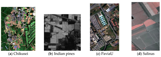
Figure 4.
Different experimental data sets. (a) Chikusei, (b) Indian pines, (c) University of Pavia, and (d) Salinas. The data set of Chikusei can be found from: http://park.itc.u-tokyo.ac.jp/sal/hyperdata/, while the data sets of Indian pines, University of Pavia and Salinas can be downloaded from: http://www.ehu.eus/ccwintco/index.php?title=Hyperspectral_Remote Sensing_Scenes.
The first hyperspectral data is Chikusei, taken by Headwall’s Hyperspectral Visible and Near-Infrared, series C (VNIR-C) imaging sensor over Chikusei, Ibaraki, Japan, in July 2014. This data set comprises 128 bands in the spectral range from 0.363 to 1.018 μm. The image consists of 540 × 420 pixels with a spatial resolution of 2.5 m/pixel, mainly including agricultural and urban areas. The second hyperspectral data is of Indian pines, acquired in 1992 by the Airborne Visible/Infrared.
Imaging Spectrometer (AVIRIS) sensor, with 224 spectral range from 0.4 to 2.5 μm. This data consists of 145 × 145 pixels with a spatial resolution of 20 m/pixel. The corrected Indian pines only has 200 bands, because 4 zero bands and 20 bands absorbed by water were removed. The third data set is the University of Pavia, obtained by Reflective Optics System Imaging Spectrometer (ROSIS) sensor, over Pavia, Northern Italy in 2003. It consists of 610 × 340 pixels with a spatial resolution of 1.3 m/pixel. There are 103 spectral bands, covering the spectral range from 0.430 to 0.838 μm. The last hyperspectral data is Salinas, which was also taken by AVIRIS in 1998 over Salinas Valley, California. This data consists of 512 × 217 pixels with a spatial resolution of 3.7 m/pixel, and 224 spectral bands are included. Similar to Indian pines, in the corrected Salinas data, 20 atmospheric and water bands were removed. In the experiments, we firstly generated the MSI and the low spatial resolution HSI, with the original hyperspectral data as the reference fusion results. The MSI was generated by down-sampling the reference image in the spectral domain using multispectral SRFs as filters. The low spatial resolution HSI was generated by an isotropic Gaussian PSF [8] with a full width at half maximum (FWHM) of the Gaussian function. Different GSD ratios, i.e., 2, 5, and 6, are used for spatial simulation in the experiments to show the performance in different conditions. After spectral and spatial simulations, band dependent Gaussian noise was added to the simulated HSI and MSI. For realistic noise conditions, a signal-to-noise ratio (SNR) of 50 dB was simulated in all bands.
The performance of fusion methods was evaluated by comparing the fusion results with the original reference images. Here, we use the following three widely used quality measures for result assessment: (1) Spectral angle mapper (SAM), (2) peak signal-to-noise ratio (PSNR), and (3) root mean square errors (RMSE) between the reconstructed H2SI and reference. In addition, our experiments are programmed in Matlab 2015b on an Intel(R) Core(TM) i7-4790HQ CPU @ 3.60GHz Computer with 16.00 GB RAM.
3.2. Analysis of the Adversarial Selection Fusion (ASF) Strategy
Compared with fusion results of BRF and UF, we analyze the effectiveness of the proposed ASF method. As analyzed before, the UF method and the BRF method can obtain two different but complementary results, thus we propose the SSQ index to synthesize these two data in an adversarial selection process. Figure 5 shows the PSNR of each band on four data sets, with different lines representing different methods.
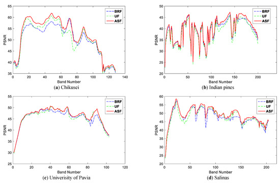
Figure 5.
Peak signal to noise ratio (PSNR) values of each band on four data sets. (a) Chikusei, (b) Indian Pines, (c) Univerisity of Pavia, and (d) Salinas. BFR, UF and ASF represent band reconstruction-based fusion, unmixing based fusion and the final adversarial selection fusion, respectively.
As shown in Figure 5, the PSNR lines of BRF and UF are crossed, which means that in some bands the BRF method performs better, but in other bands the UF method performs better. However, the PSNR of the ASF result is higher than both the UF and BRF in almost all of the bands. This means that the SSQ index based adversarial selection strategy can effectively complete the synthesis for these two preliminary data. Taking Figure 5a as an example, it can be seen that in the 15–60 bands, the UF method performs better than the BRF method, while the situation is exactly opposite in the 65–80 bands. However, in all bands, the final ASF result is the same or better than both of them. These results demonstrate the potential of our adversarial selection strategy and the effectiveness of the SSQ index.
More objective results are shown in Table 1. In this table, the average SAM of all pixels, average PSNR of all bands and RMSE between the reconstructed H2SI and reference on four data sets are listed, and the best results are written in bold. As we can see, the SAM performance of the UF method is better than the BRF method, while the PSNR performance of the BRF method is better than the UF method. However, the final ASF result is better than both of these two preliminary fusion results, which strongly proves the effectiveness of our ASF method. As stated in Section 2.3, the UF method can only preserve the spatial correlation in MSI, while the BRF method can only keep the spectral correlation in HSI, which means these two methods solve the HSI–MSI fusion problem from two different but complementary aspects. With the SSQ index as guidance, the ASF method choose the parts with respective high scores, thus the final fusion result performs better than both UF and BRF.

Table 1.
Comparison of average spectral angle mapper (SAM), average PSNR and root mean square errors (RMSE) on four data sets.
3.3. Experiments Results
To verify the effectiveness of the proposed method, several well-known HSI–MSI fusion methods, including two pan-sharpening based methods, i.e., Gram–Schmidt adaptive [34] (GSA) and smoothing filtered-based intensity modulation [35] (SFIM), and two spectral unmixing based methods, i.e., Lanaras’s method [26] and Hysure [23], are used as compared methods. Meanwhile, we use RMSE, the average SAM of all pixels, and the PSNR of all bands as the indexes to evaluate the quality of these fusion results.
The visual quality comparison is shown in Figure 6, Figure 7, Figure 8 and Figure 9. We adopted the spectral angle mapper (SAM) to demonstrate the differences of fusion results from different methods. In these maps, the warmer colors mean the larger spectral angle errors between fusion results and the ground truth. All results are demonstrated in the same conditions to ensure fairness of the experiments. The figures show the reference grayscale and the SAM of fusion results from different methods, i.e., GSA, HySure, lanaras’s method, SFIM, and our methods including BRF, UF, and ASF.
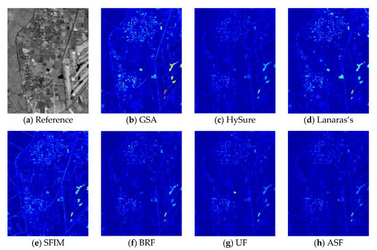
Figure 6.
SAM map of different methods on Chikusei. (a) Grayscale image of Chikusei, (b) SAM map of Gram-Schmidt adaptive (GSA), (c) SAM map of HySure, (d) SAM map of Lanaras’s method, (e) SAM map of smoothing filtered-based intensity modulation (SFIM), (f) SAM map of BRF, (g) SAM map of UF, (h) SAM of ASF. The warmer colors indicate the larger spectral angle errors.
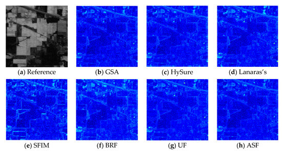
Figure 7.
SAM map of different methods on Indian pines. (a) Grayscale image of Indian pines, (b) SAM map of GSA, (c) SAM map of HySure, (d) SAM map of Lanaras’s method, (e) SAM map of SFIM, (f) SAM map of BRF, (g) SAM map of UF, (h) SAM of ASF. The warmer colors indicate larger spectral angle errors.
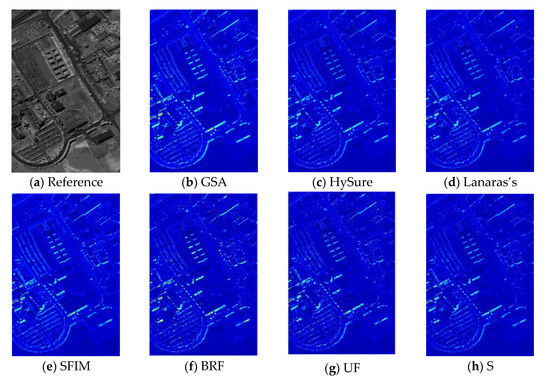
Figure 8.
SAM map of different methods on University of Pavia. (a) Grayscale image of University of Pavia, (b) SAM map of GSA, (c) SAM map of HySure, (d) SAM map of Lanaras’s method, (e) SAM map of SFIM, (f) SAM map of BRF, (g) SAM map of UF, (h) SAM of ASF. The warmer colors indicate the larger spectral angle errors.
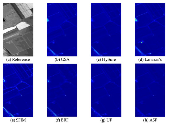
Figure 9.
SAM map of different methods on Salinas. (a) Grayscale image of Salinas, (b) SAM map of GSA, (c) SAM map of HySure, (d) SAM map of Lanaras’s method, (e) SAM map of SFIM, (f) SAM map of BRF, (g) SAM map of UF, (h) SAM of ASF. The warmer colors indicate the larger spectral angle errors.
As for the data sets of Chikusei, Salinas, and the University of Pavia, our ASF method can acquire the best fusion results. Specially, in Figure 6; Figure 9, the spectral angel errors of the ASF method was obviously smaller than other methods. This is due to the comprehensive consideration of both spectral correlation in HSI and spatial correlation in MSI. As shown in Figure 6, some pixels with large spectral angle errors in the BRF method can be better reconstructed in UF method, while the BRF method performs better than the UF method on some other pixels. As for ASF, it effectively combines the good aspects of the BRF and UF methods. On the Indian pines, GSA performs better than other methods. This is because the GSD ratio of Indian pines in our experiments is 2, smaller than the other data sets, and GSA is suitable for the lower GSD ratio. When the GSD ratio is large such as 5 or 6, the performance of the GSA is not good as Figure 6, Figure 8 and Figure 9 show. The performance of Lanaras’s method is slightly better than GSA, but worse than our ASF method, which indicates that simple spectral unmixing towards HSI and MSI cannot achieve perfect results. HySure has achieved good results on the data sets of Chikusei and Salinas, but the performances on the other two data sets are not good, which shows that the vector-total-variation regularization in GySure is not very versatile. In summary, our ASF method acquires better fusion performance compared to other methods due to the considerations of both spectral and spatial dimensions.
In addition, some objective metrics are listed to prove the effectiveness of our approach. Table 2 shows the average SAM, PSNR, and RMSE values, including four data sets and five different methods. The SAM values are the averages of all pixels, while the PSNR values are the averages of all bands. In the three tables, the best results for each index are written in bold letters. As we can see from these results, our proposed method performs better than other well-known and effective methods in most cases, except Indian pines. As mentioned above, GSA performs better when the GSD ratio is smaller. Our proposed method achieves better results owing to the consideration of both spatial correlations in MSI and the spectral correlation in HSI. As Table 1 shows, in some occasions where the UF methods cannot work effectively, the BRF method may make up for this. Moreover, the SSQ index based adversarial selection strategy effectively synthesizes these two complementary aspects, leading to the fine fusion results as the tables show.
Table 2.
Assessment Results of Average SAM (in degrees), Average PSNR (in decibels) and RMSE Values.
4. Conclusions
In this paper, a new adversarial HSI–MSI fusion method is proposed, taking both the spectral and spatial correlations into account. Considering the spatial correlation contained in MSI, the UF method is adopted for a preliminary fusion result. In order to preserve the spectral correlation contained in HSI, the BRF method is proposed, which reconstructs another preliminary fusion result by the product of band image dictionary and reconstruction coefficients. In addition, Spectral Spatial Quality (SSQ) is designed as the guidance for subsequent adversarial selection processes. The performance comparison of UF, BRF, and the final ASF has strongly proved the effectiveness of the adversarial selection strategy. Compared to other classical fusion methods, SAM and PSNR performance of the ASF method has achieved significant improvement due to the comprehensive considerations of spatial and spectral correlation. Experiments on four real data sets indicate the effectiveness of our proposed ASF method.
Author Contributions
X.K.L. performed the experiments and wrote the manuscript. J.Y. proposed and discussed the original idea and revised the manuscript. X.Y.L. discussed the original idea and revised the manuscript. X.J. gave some comments and ideas for the work.
Funding
This research was funded by National Natural Science Foundation of China (Grant 41471278 and 41871240).
Conflicts of Interest
The authors declare no conflict of interest.
References
- Bendoumi, M.A.; He, M.; Mei, S. Hyperspectral image resolution enhancement using high-resolution multispectral image based on spectral unmixing. IEEE Trans. Geosci. Remote Sens. 2014, 52, 6574–6583. [Google Scholar] [CrossRef]
- Yin, J.; Gao, C.; Jia, X. A new target detector for hyperspectral data using Cointegration Theory. IEEE J. Sel. Top. Appl. Earth Observ. Remote Sens. 2013, 6, 638–643. [Google Scholar] [CrossRef]
- Alparone, L.; Wald, L.; Chanussot, J.; Thomas, C.; Gamba, Y.; Bruce, L.M. Comparison of pansharpening algorithms: Outcome of the 2006 GRS-S data fusion contest. IEEE Trans. Geosci. Remote Sens. 2007, 45, 3012–3021. [Google Scholar] [CrossRef]
- Yin, H. A Joint Sparse and Low-Rank Decomposition for Pansharpening of Multispectral Images. IEEE Trans. Geosci. Remote Sens. 2017, 55, 3545–3557. [Google Scholar] [CrossRef]
- Vivone, G.; Alparone, L.; Chanussot, J.; Mura, M.D.; Garzelli, A.; Licciardi, G.; Restaino, R.; Wald, L. A critical comparison among pansharpening algorithms. IEEE Trans. Geosci. Remote Sens. 2015, 53, 2565–2586. [Google Scholar] [CrossRef]
- Zhu, X.X.; Grohnfeldt, C.; Bamler, R. Exploiting joint sparsity for pansharpening: The J-SparseFI algorithm. IEEE Trans. Geosci. Remote Sens. 2016, 54, 2664–2681. [Google Scholar] [CrossRef]
- Luo, X.Y.; Zhou, L.Y.; Shi, X.F.; Wan, H.; Yin, J.H. Spectral mapping based on panchromatic block structure analysis. IEEE Access. 2018, 6, 40354–40364. [Google Scholar] [CrossRef]
- Yokoya, N.; Grohnfeldt, C.; Chanussot, J. Hyperspectral and multispectral data fusion: A comparative review of the recent literature. IEEE Geosci. Remote Sens. Mag. 2017, 5, 29–56. [Google Scholar] [CrossRef]
- Gomez, R.; Jazaeri, A.; Kafatos, M. Wavelet-based hyperspectral and multi-spectral image fusion. Proc. SPIE-Int. Soc. Opt. Eng. 2001, 4383, 36–42. [Google Scholar]
- Chan, R.H.; Chan, T.F.; Shen, L.; Shen, Z. Wavelet algorithms for high-resolution image reconstruction. SIAM J. Sci. Comput. 2003, 24, 1408–1432. [Google Scholar] [CrossRef]
- Atkinson, I.; Kamalabadi, F.; Jones, D.L. Wavelet-based hyperspectral image estimation. In Proceedings of the IEEE International Geoscience and Remote Sensing Symposium, Toulouse, France, 21–25 July 2003; pp. 743–745. [Google Scholar]
- Chen, Z.; Pu, H.; Wang, B.; Jiang, G.M. Fusion of hyperspectral and multispectral images: A novel framework based on generalization of pan-sharpening methods. IEEE Geosci. Remote Sens. Lett. 2014, 11, 1418–1422. [Google Scholar] [CrossRef]
- Zhu, Z.; Yin, H.; Chai, Y.; Li, Y.; Qi, G. A novel multi-modality image fusion method based on image decomposition and sparse representation. Inf. Sci. 2018, 432, 516–529. [Google Scholar] [CrossRef]
- Grohnfeldt, C.; Zhu, X.X.; Bamler, R. Jointly sparse fusion of hyperspectral and multispectral imagery. In Proceedings of the 2013 IEEE International Geoscience and Remote Sensing Symposium-IGARSS, Melbourne, VIC, Australia, 21–26 July 2013; pp. 1–4. [Google Scholar]
- Grohnfeldt, C.; Zhu, X.X.; Bamler, R. The J-SparseFI-HM hyperspectral resolution enhancement method now fully automated. In Proceedings of the IEEE Workshop on Hyperspectral Image and Signal Processing: Evolution in Remote Sensing (WHISPERS), Lausanne, Switzerland, 24–27 June 2014; pp. 1–4. [Google Scholar]
- Selva, M.; Aiazzi, B.; Butera, F.; Chiarantini, L.; Baronti, S. Hyper-sharpening: A first approach on SIM-GA data. IEEE J. Sel. Top. Appl. Earth Observ. Remote Sens. 2015, 8, 3008–3024. [Google Scholar] [CrossRef]
- Berné, O.; Helens, A.; Pilleri, P.; Joblin, C. Non-negative matrix factorization pansharpening of hyperspectral data: An application to mid-infrared astronomy. In Proceedings of the IEEE Workshop on Hyperspectral Image and Signal Processing: Evolution in Remote Sensing (WHISPERS), Reykjavik, Iceland, 14–16 June 2010; pp. 1–4. [Google Scholar]
- Yokoya, N.; Yairi, T.; Iwasaki, A. Coupled non-negative matrix factorization (CNMF) for hyperspectral and multispectral data fusion: Application for pasture classification. In Proceedings of the 2011 IEEE International Geoscience and Remote Sensing Symposium, Vancouver, BC, Canada, 24–29 July 2011; pp. 1779–1782. [Google Scholar]
- Yokoya, N.; Yairi, T.; Iwasaki, A. Coupled nonnegative matrix factorization unmixing for hyperspectral and multispectral data fusion. IEEE Trans. Geosci. Remote Sens. 2012, 50, 528–537. [Google Scholar] [CrossRef]
- Akhtar, N.; Shafait, F.; Mian, A. Sparse spatio-spectral representation for hyperspectral image super-resolution. In Proceedings of the European Conference on Computer Vision, Zurich, Switzerland, 6–12 September 2014; pp. 63–78. [Google Scholar]
- Kawakami, R.; Wright, J.; Tai, Y.; Matsushita, Y.; Ben-Ezra, M.; Ikeuchi, K. High-resolution hyperspectral imaging via matrix factorization. In Proceedings of the IEEE Conference on Computer Vision and Pattern Recognition (CVPR), Colorado Springs, CO, USA, 20–25 June 2011; pp. 2329–2336. [Google Scholar]
- Wycoff, E.; Chan, T.H.; Jia, K.; Ma, W.K.; Ma, Y. A nonnegative sparse promoting algorithm for high resolution hyperspectral imaging. In Proceedings of the IEEE International Conference on Acoustics, Speech and Signal Processing (ICASSP), Vancouver, BC, Canada, 26–31 May 2013; pp. 1409–1413. [Google Scholar]
- Simões, M.; Dias, J.B.; Almeida, L.; Chanussot, J. A convex formulation for hyperspectral image superresolution via subspace-based regularization. IEEE Trans. Geosci. Remote Sens. 2015, 53, 3373–3388. [Google Scholar] [CrossRef]
- Yi, C.; Zhao, Y.; Yang, J.; Kong, G. Joint hyperspectral superresolution and unmixing with interactive feedback. IEEE Trans. Geosci. Remote Sens. 2017, 55, 3823–3834. [Google Scholar] [CrossRef]
- Roozbeh, R.; Hassan, G. Spectral unmixing of hyperspectral imagery using multilayer NMF. IEEE Geosci. Remote Sens. Lett. 2015, 12, 38–42. [Google Scholar]
- Lanaras, C.; Baltsavias, E.; Schindler, K. Hyperspectral super-resolution by coupled spectral unmixing. In Proceedings of the IEEE International Conference on Computer Vision, Beijing, China, 7–20 October 2005; pp. 3586–3594. [Google Scholar]
- Heinz, D.C.; Chang, C.I. Fully constrained least squares linear spectral mixture analysis method for material quantification in hyperspectral imagery. IEEE Trans. Geosci. Remote Sens. 2001, 39, 529–545. [Google Scholar] [CrossRef]
- Yuan, Y.; Zhu, G.; Wang, Q. Hyperspectral band selection by multitask sparsity pursuit. IEEE Trans. Geosci. Remote Sens. 2015, 53, 631–644. [Google Scholar] [CrossRef]
- Yin, J.; Sun, J.; Jia, X. Sparse analysis based on generalized Gaussian model for spectrum recovery with compressed sensing theory. IEEE J. Sel. Top. Appl. Earth Observ. Remote Sens. 2015, 8, 2752–2759. [Google Scholar]
- Sun, W.; Zhang, L.; Du, B.; Li, W.; Lai, Y. Band selection using improved sparse subspace clustering for hyperspectral imagery classification. IEEE J. Sel. Top. Appl. Earth Observ. Remote Sens. 2015, 8, 2784–2797. [Google Scholar] [CrossRef]
- Yin, J.H.; Qv, H.; Luo, X.Y.; Jia, X.P. Segment-oriented depiction and analysis for hyperspectral image data. IEEE Trans. Geosci. Remote Sens. 2017, 55, 3982–3996. [Google Scholar] [CrossRef]
- Liu, X.; Xia, W.; Wang, B.; Zhang, L. An approach based on constrained nonnegative matrix factorization to unmix hyperspectral data. IEEE Trans. Geosci. Remote Sens. 2011, 49, 757–772. [Google Scholar] [CrossRef]
- Lee, D.D.; Seung, H.S. Learning the parts of objects by nonnegative matrix factorization. Nature 1999, 401, 788–791. [Google Scholar] [CrossRef] [PubMed]
- Aiazzi, B.; Baronti, S.; Selva, M. Improving component substitution pansharpening through multivariate regression of MS+Pan data. IEEE Trans. Geosci. Remote Sens. 2007, 45, 3230–3239. [Google Scholar] [CrossRef]
- Liu, J.G. Smoothing filter-based intensity modulation: A spectral preserve image fusion technique for improving spatial details. Int. J. Remote Sens. 2000, 21, 3461–3472. [Google Scholar] [CrossRef]
© 2019 by the authors. Licensee MDPI, Basel, Switzerland. This article is an open access article distributed under the terms and conditions of the Creative Commons Attribution (CC BY) license (http://creativecommons.org/licenses/by/4.0/).