Refined Two-Stage Programming-Based Multi-Baseline Phase Unwrapping Approach Using Local Plane Model

Abstract

The problem of phase unwrapping (PU) in synthetic aperture radar (SAR) interferometry (InSAR) is caused by the measured range differences being ambiguous with the wavelength. Therefore, multi-baseline (MB) is a key processing step of MB InSAR. Compared with the traditional single-baseline (SB) PU, MB PU is advantageous in solving steep terrain due to its ability to break through the constraint of the phase continuity assumption. However, the accuracy of most of the existing MB PU methods is still limited to its mathematical foundation, i.e., the Chinese remainder theorem (CRT) is too sensitive to measurement bias. To solve this issue, this paper presents a refined algorithm based on the two-stage programming MB PU approach (TSPA) proposed by H. Yu. The significant advantage of the refined TSPA method (abbreviated as LPM-TSPA) is that it improves the performance of stage 1 of TSPA through assuming terrain height surface in the neighborhood pixels can be approximated by a plane to combine more information of the interferometric phase in the local region to estimate the ambiguity number gradient. The experiment results indicate that the LPM-TSPA method can significantly improve the accuracy of the MB PU solution.

1. Introduction

Synthetic aperture radar (SAR) interferometry (InSAR) has created a new class of radar data for remote sensing applications that has significantly developed over the last couple of decades. Most of the InSAR-based applications, e.g., topographic mapping and deformation measuring, typically rely on the phase unwrapping (PU) technique, because InSAR can directly extract only the absolute phase modulo $2\pi$, i.e., wrapped phase. Figure 1a shows an example of the filtered and flattened realistic InSAR wrapped phase image (called interferogram in the rest of this paper) from the Etna volcano, Italy. Figure 1b is the coherence of Figure 1a, which reflects the goodness of each pixel (the pixel value in Figure 1b is from 0 (worst) to 1 (best)). Under this condition, the technique of phase-ambiguity removal, i.e., PU, is an indispensable processing step of InSAR. It is known that the traditional single-baseline (SB) PU is an ill-posed problem, because there are two unknowns, i.e., absolute phase and integer ambiguity, need to be solved with one equation (the absolute phase can be directly converted to the topographic information). However, the MB PU is well-posed through making use of the baseline diversity to significantly increase the ambiguity intervals of interferometric phases. To be specific, MB PU does not need to obey the Itoh condition (also known as phase continuity assumption) [1]. A statistic for the journal and conference publications of the MB PU is given in [2], and from 1997 to 2017, the average annual growth rate of the number of papers published is about $42.83\%$. The exponential growth trend of the number of papers reveals the rapid surge of study of MB PU.

In the past two decades, various MB PU methods with different advantages have been put forward, many of which based on statistical framework or Chinese remainder theorem (CRT). The MB PU methods based on statistical framework use the InSAR probability density function (PDF) to establish the maximum likelihood (ML) or maximum a posteriori (MAP), so they are also called the parametric-based MB PU methods [1,2]. Ref. [3] proposed a MB PU method with using a ML formulation. Ref. [4] presented an unwrapping method based on a ML estimation technique. Ref. [5] addressed the derivation of the phase difference-based ML PU algorithm. Ref. [6] proposed maximum a posteriori (MAP) PU method to reconstruct terrain heights. Ref. [7] presented a Markovian approach to solve the multichannel PU problem. Ref. [8] is a review paper of the ML- and MAP-based methods. Furthermore, the height estimation accuracy between the ML- and MAP-based methods is analyzed in [9]. Contrast to parametric-based MB PU methods, nonparametric-based MB PU methods have also been put forward, which obtain the PU solution by translating the MB PU problem to an unsupervised-learning problem, i.e., cluster-analysis (CA) problem [2]. A fast CA-based MB PU method was proposed by [10], and was improved in [11,12]. In addition, many MB PU methods base on CRT were presented as well. Ref. [13] described an iterative MB PU method which starts at the shortest baseline and proceeds to longer and longer baselines. Ref. [14] presented a MB PU method based on 3-D Kalman filtering. The wavelet approach was applied on MB PU in [15]. Ref. [16] proposed three basic MB PU methods, i.e., CRT method, projection method and linear combination method. Ref. [17] presented a method to reconstruct the digital elevation model (DEM) using the closed-form robust CRT. To improve the robustness to noise, Ref. [18] put forward a MB PU method based on the mix-integer optimization model. Ref. [19] presented an alternative algorithm for PU where only a subset of data from the wrapped phase map is used to reconstruct the unwrapped phase map as a linear combination of radial basis functions (RBF’s) so that the conventional PU step is not used.

In summary, most of the aforementioned methods suffer from poor measurement bias robustness (the measurement bias could be potentially caused by atmospheric artifact, surface deformation, or system noise). Moreover, the ML-, MAP-, and CA-based MB PU methods are all derived from machine learning techniques, so they usually include several parameters without clear PU meanings, which needs the extra information to decide. In this case, it will set some limits on the application scope of these MB PU methods. To solve these issues, Ref. [1] proposed a two-stage programming-based MB PU method (TSPA) that builds a link between SB and MB PUs. In the first stage, according to the formulation of CRT, TSPA estimates the ambiguity number difference between neighboring pixels using multiple interferograms with different baseline lengths. Afterwards, the final PU result can be obtained by using the SB PU framework. Compared with most of the aforementioned existing MB PU methods, the fundamental contributions of the TSPA method are listed as follows. To begin with, TSPA uses the information of all the pixels in the interferogram to improve the noise robustness [1]. In addition, since TSPA makes the connection between SB and MB PUs, the framework of TSPA can be transplanted into most of the SB PU-based InSAR techniques, e.g., two-pass and three-pass differential InSAR (DInSAR) techniques [20]. Also, many existing classical SB PU concepts can be transplanted into MB domain. However, because stage 1 of TSPA is dependent on CRT, which is too sensitive to measurement bias that is potentially caused by atmospheric artifact, surface deformation, or system noise, there is still room to further advance TSPA through refining the performance of stage 1. To further improve the noise robustness of the original TSPA method, a refined TSPA MB PU method based on local plane model (abbreviated as LPM-TSPA method) is proposed in this paper. The LPM-TSPA method improves the performance of stage 1 of TSPA through assuming terrain height surface in the neighborhood pixels can be approximated by a plane to combine more information of the interferometric phase in the local region to estimate the ambiguity number gradient. In this paper, the basic principle of the original TSPA is reviewed first, in which we discuss why there is still room to further advance TSPA through refining the performance of stage 1 of TSPA. Then, we design a local plane model, which introduces a relation among the profile at the given position and that in neighboring positions, to combine more wrapped phase information to estimate the ambiguity number gradient. Based on this model, the LPM-TSPA method with better noise robustness is proposed. The experiment results indicate that the LPM-TSPA method can significantly improve the PU accuracy of the original TSPA method.

The rest of this paper is organized as follows. Section 2 reviews the TSPA method and analyzes its advantages and disadvantages. In Section 3, the LPM-TSPA method is described in detail. Then, in Section 4, the proposed method is validated by a set of simulated and realistic MB InSAR datasets and the results are discussed. Finally, Section 5 concludes this paper.

2. Review and Analysis of TSPA

In this section, we will review the original TSPA method under the dual-baseline (DB) case. For the MB case, the readers can refer to [1]. If the size of the interferograms obtained by the DB InSAR system is $m\times n$ and the pixel of the ith row and jth column in the interferograms is referred as pixel $(i,j)$. The InSAR measurement of a pixel can be given by

$${\phi }_r(i,j)={\psi }_r(i,j)-2\pi ·k_r(i,j),$$

(1)

where ${\phi }_r(i,j)$, ${\psi }_r(i,j)$ and integer $k_r(i,j)$ are the wrapped phase, absolute phase, and ambiguity number of the pixel $(i,j)$ in interferogram $r(r=1,2)$, respectively. ${\phi }_r(i,j)$ can be measured by the DB InSAR system, but ${\psi }_r(i,j)$ and $k_r(i,j)$ are the unknowns that need to be solved. If the ambiguity number $k_r(i,j)$ of each pixel can be solved, ${\psi }_r(i,j)$ that contains the terrain information can be obtained through Equation (1). The absolute phases of the two interferograms can be combined by using the baseline lengths such as [1]

$$B_2·({\phi }_1(i,j)+2\pi ·k_1(i,j))=B_1·({\phi }_2(i,j)+2\pi ·k_2(i,j)),$$

(2)

where $B_1$ and $B_2$ represent two different normal baseline (or perpendicular baseline) lengths [8,11]. In the rest of this paper, normal baseline length is shortened as baseline length. According to Equation (2), the TSPA method establishes the relationship of gradient information in different interferograms with different baselines as shown in Equations (3) and (4)

$$B_2·({\Delta }_{{\phi }_1}^x(i,j)+2\pi ·{\Delta }_{k_1}^x(i,j))=B_1·({\Delta }_{{\phi }_2}^x(i,j)+2\pi ·{\Delta }_{k_2}^x(i,j)),$$

(3)

$$B_2·({\Delta }_{{\phi }_1}^y(i,j)+2\pi ·{\Delta }_{k_1}^y(i,j))=B_1·({\Delta }_{{\phi }_2}^y(i,j)+2\pi ·{\Delta }_{k_2}^y(i,j)),$$

(4)

where ${\Delta }_{{\phi }_r}^x(i,j)={\phi }_r(i,j+1)-{\phi }_r(i,j)$, ${\Delta }_{{\phi }_r}^y(i,j)={\phi }_r(i+1,j)-{\phi }_r(i,j)$, ${\Delta }_{k_r}^x(i,j)=k_r(i,j+1)-k_r(i,j)$, ${\Delta }_{k_r}^y(i,j)=k_r(i+1,j)-k_r(i,j)$, $r=1,2$. The superscript x and y represent the adjacent relationship on horizontal and vertical directions of adjacent pixels, respectively. ${\Delta }_{{\phi }_r}^x(i,j)$ and ${\Delta }_{{\phi }_r}^y(i,j)$ are the wrapped phase differences between adjacent pixels of interferogram r. ${\Delta }_{k_r}^x(i,j)$ and ${\Delta }_{k_r}^y(i,j)$ are the ambiguity number gradient between adjacent pixels of interferogram r. According to CRT, we can obtain the solution to Equations (3) and (4) under some special combination of the baseline lengths (because ${\Delta }_{k_r}^x(i,j)$ and ${\Delta }_{k_r}^y(i,j)$ are integer) [1]. Equations (3) and (4) can be solved by the optimization model shown in (5) and (6)

$$\begin{array}{c}\hfill \left\{\begin{array}{cc}arg& \underset{{\widehat{\Delta }}_{k_1}^x(i,j),{\widehat{\Delta }}_{k_2}^x(i,j)}{min}{\zeta }^x(i,j)\\ s.t.& {\widehat{\Delta }}_{k_r}^x(i,j)\in integer,r=1,2.\end{array}\right.\end{array}$$

(5)

$$\begin{array}{c}\hfill \left\{\begin{array}{cc}arg& \underset{{\widehat{\Delta }}_{k_1}^y(i,j),{\widehat{\Delta }}_{k_2}^y(i,j)}{min}{\zeta }^y(i,j)\\ s.t.& {\widehat{\Delta }}_{k_r}^y(i,j)\in integer,r=1,2.\end{array}\right.\end{array}$$

(6)

where ${\widehat{\Delta }}_{k_r}^x(i,j)$ and ${\widehat{\Delta }}_{k_r}^y(i,j)(r=1,2)$ are the decision variables, and the objective functions (i.e., ${\zeta }^x(i,j)$ and ${\zeta }^y(i,j)$) of Equations (5) and (6) are defined in Equations (7) and (8)

$${\zeta }^x(i,j)=|B_2·({\Delta }_{{\phi }_1}^x(i,j)+2\pi ·{\widehat{\Delta }}_{k_1}^x(i,j))-B_1·({\Delta }_{{\phi }_2}^x(i,j)+2\pi ·{\widehat{\Delta }}_{k_2}^x(i,j))|,$$

(7)

$${\zeta }^y(i,j)=|B_2·({\Delta }_{{\phi }_1}^y(i,j)+2\pi ·{\widehat{\Delta }}_{k_1}^y(i,j))-B_1·({\Delta }_{{\phi }_2}^y(i,j)+2\pi ·{\widehat{\Delta }}_{k_2}^y(i,j))|.$$

(8)

It can be seen that ${\zeta }^x(i,j)$ and ${\zeta }^y(i,j)$ are the CRT biases, so Equations (5) and (6) are to find the ambiguity number gradient (i.e., ${\widehat{\Delta }}_{k_r}^x(i,j)$ and ${\widehat{\Delta }}_{k_r}^y(i,j)$) with minimum CRT biases [1]. Based on the gradient information obtained by Equations (5)–(8), TSPA uses the framework of the $L^1$-norm SB PU to respectively obtain the final PU result of each interferogram by Equation (9),

$$\begin{array}{c}\hfill \left\{\begin{array}{cc}min& {\displaystyle \sum _{i=1}^m}{\displaystyle \sum _{j=1}^{n-1}}{\omega }_r^x(i,j)·\mid k_r(i,j+1)-k_r(i,j)-{\widehat{\Delta }}_{k_r}^x(i,j)\mid +\hfill \\ & {\displaystyle \sum _{i=1}^{m-1}}{\displaystyle \sum _{j=1}^n}{\omega }_r^y(i,j)·\mid k_r(i+1,j)-k_r(i,j)-{\widehat{\Delta }}_{k_r}^y(i,j)\mid \hfill \\ s.t.& k_r(i,j)\in integer,r=1,2.\end{array}\right.\end{array}$$

(9)

where ${\omega }_r^x(i,j)$ and ${\omega }_r^y(i,j)$ are the weights that can usually be obtained by using any kind of quality maps of the input interferograms [1], and $k_r(i,j)$ is the decision variable.

As described in Section 1, many important SB PU concepts can be transplanted into MB domain through using the framework of TSPA [1]. For example, under the framework of TSPA, we can define the MB residue, i.e., the loop integration value of the gradients obtained by Equations (5) and (6) of any $2\times 2$ neighboring pixels. 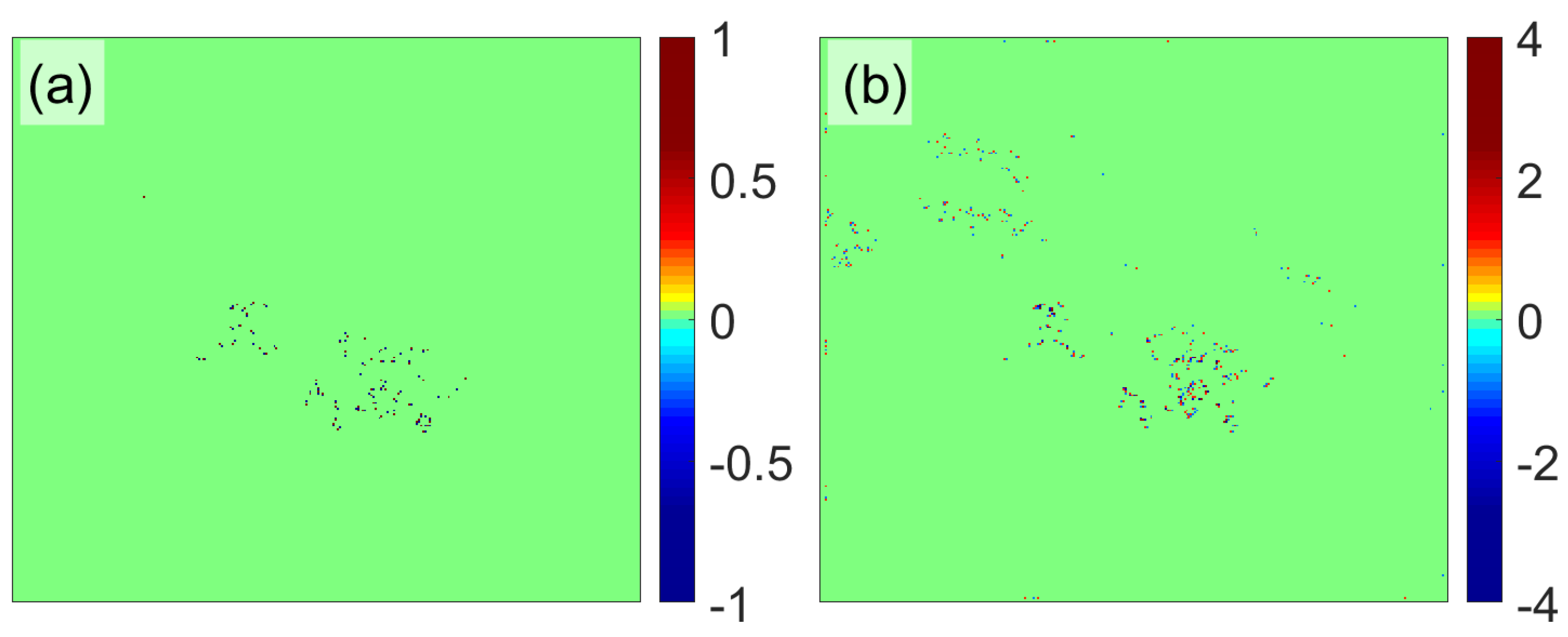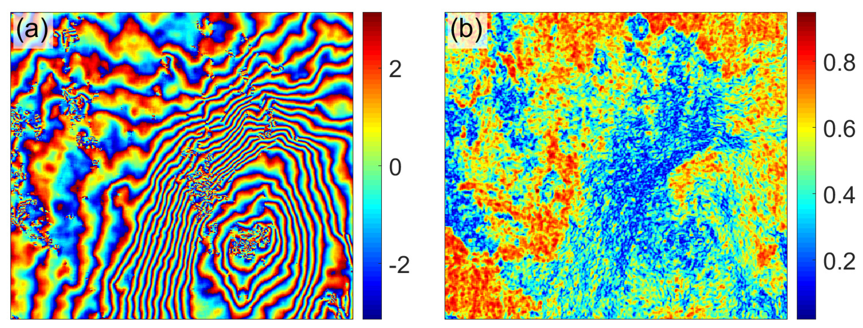Because the MB PU does not follow the SB PU using the Itoh condition to estimate the gradient information, the MB residue polarity is $\pm N$, $N\in$ Integer, but that in SB is ±1 [20]. It can be seen that the TSPA method consists of two stages. In stage 1, the ambiguity number gradient is estimated according to the CRT formulation. In stage 2, the final PU result of each interferogram is obtained by the framework of the SB $L^1$-norm PU method. However, as described, CRT is too sensitive to measurement bias that is potentially caused by atmospheric artifact, surface deformation, or system noise, so the gradient information obtained in stage 1 will be very noisy. For example, Figure 2a,b are two realistic interferograms with different baseline lengths (6.40 m and 40.29 m respectively). Other system interferometric parameters of Figure 2a,b are the same to those of the TerraSAR-X MB InSAR dataset employed in Experiment 2. Figure 2c,d are the SB residue distributions of Figure 2a,b. Figure 2e,f are the MB residue distributions of Figure 2a,b obtained by the TSPA method. The statistical information of Figure 2c–f is shown in

Table 1. Statistical Information of Residue Distribution.

		SB				MB
	Figure 2c		Figure 2d		Figure 2e		Figure 2f
Polarity range of the residues	[−1, 1]		[−1, 1]		[−1, 1]		[−8, 7]
Number of the residues	144		175		146		3494
Total polarity of the residues	144		175		146		4277

.

Table 1 indicates that although the MB gradient information does not need to obey the Itoh condition (the polarity of MB residue is not restricted as $\pm 1$), it is much more noisy than that under the SB situation (because the SB residue distribution is sparser and its total polarity is lower). In other words, although TSPA uses the global information to prevent the influence of the noise, there is still room to further advance TSPA through refining the performance of stage 1.

3. LPM-TSPA Method

From the discussion in Section 2, we know that our object is to design a method to help the CRT to resist the influence of noise from stage 1 of TSPA. From Equation (5), we can see that only the information of the four pixels from two interferograms, i.e., ${\phi }_1(i,j+1)$, ${\phi }_1(i,j)$, ${\phi }_2(i,j+1)$ and ${\phi }_2(i,j)$, are used to estimate ${\widehat{\Delta }}_{k_1}^x(i,j)$ and ${\widehat{\Delta }}_{k_2}^x(i,j)$. It is not difficult to believe that better performance can surely be achieved if more information of the interferometric phase can be combined to estimate the ambiguity number gradient. In other words, if we introduce some relation among the deformation values in an assigned cluster of neighboring pixels so that more pixels will be jointed in stage 1, the effect of noise on the ambiguity number gradient estimation will be reduced. The basic idea for obtaining such a solution is presented as follows.

We know that the absolute phase corresponds to the elevation of topography surface. Under this condition, if we take a small enough local area on the surface, such as a rectangular window, we can assume that the height surface of this rectangular window can be approximated by a plane. Through using the plane equation, we will have

$${\psi }_r(i^{\prime },j^{\prime })={\Delta }_{{\psi }_r}^y(i,j)·(i^{\prime }-i)+{\Delta }_{{\psi }_r}^x(i,j)·(j^{\prime }-j)+{\psi }_r(i,j),(i^{\prime },j^{\prime })\in \mathsf{\Omega }(i,j)$$

(10)

where $\mathsf{\Omega }(i,j)$ is the set in which the elements are points within the plane containing $(i,j)$. ${\Delta }_{{\psi }_r}^x(i,j)$, ${\Delta }_{{\psi }_r}^y(i,j)$ and ${\psi }_r(i,j)$ are the parameters constructing the local plane, and ${\Delta }_{{\psi }_r}^x(i,j)={\psi }_r(i,j+1)-{\psi }_r(i,j)$, ${\Delta }_{{\psi }_r}^y(i,j)={\psi }_r(i+1,j)-{\psi }_r(i,j)$. We can see that the relation among pixels built by Equation (10) could potentially joint all the pixels in the rectangular window. Hence, we will refine stage 1 of the TSPA method through assuming terrain height surface in the neighborhood pixels can be approximated by a plane to combine more information of the interferometric phase in the local region to estimate the ambiguity number gradient.

In the following, through using Equation (10), the model of the LPM-TSPA method under the DB case is described in detail, and that of the MB case is given in the Appendix. Taking a rectangular window centered on pixel $(i,j)$, we assume that the window size is $(2p+1)\times (2q+1)$, where p and q are positive integers (how to choose the values of p and q will be discussed later). For a given $(i,j)$, define a set $S=\left\{(i^{\prime },j^{\prime })\right|i^{\prime }=i-p,\dots ,i+p;j^{\prime }=j-q,\dots ,j+q\}$, then, two refined optimization models for the ambiguity number gradient estimation will be shown in Equations (11) and (12).

$$\begin{array}{c}\hfill \left\{\begin{array}{cc}arg& \underset{{\widehat{\Delta }}_{k_1}^x(i,j),{\widehat{\Delta }}_{k_2}^x(i,j)}{min}{Z}^x(i,j)\\ s.t.& {\widehat{\Delta }}_{k_r}^x(i,j)\in integer,r=1,2.\end{array}\right.\end{array}$$

(11)

$$\begin{array}{c}\hfill \left\{\begin{array}{cc}arg& \underset{{\widehat{\Delta }}_{k_1}^y(i,j),{\widehat{\Delta }}_{k_2}^y(i,j)}{min}{Z}^y(i,j)\\ s.t.& {\widehat{\Delta }}_{k_r}^y(i,j)\in integer,r=1,2.\end{array}\right.\end{array}$$

(12)

In Equations (11) and (12), the new objective functions $Z^x(i,j)$ and $Z^y(i,j)$ are defined as

$$Z^x(i,j)=\sum _{(i^{\prime },j^{\prime })\in S}{\zeta }^x(i^{\prime },j^{\prime }),p+1\le i\le m-p,q+1\le j\le n-q-1,$$

(13)

$$Z^y(i,j)=\sum _{(i^{\prime },j^{\prime })\in S}{\zeta }^y(i^{\prime },j^{\prime }),p+1\le i\le m-p-1,q+1\le j\le n-q.$$

(14)

${\zeta }^x(i^{\prime },j^{\prime })$ and ${\zeta }^y(i^{\prime },j^{\prime })$ in Equations (13) and (14) are

$${\zeta }^x(i^{\prime },j^{\prime })=|B_2·({\Delta }_{{\phi }_1}^x(i^{\prime },j^{\prime })+2\pi ·{\widehat{\Delta }}_{k_1}^x(i^{\prime },j^{\prime }))-B_1·({\Delta }_{{\phi }_2}^x(i^{\prime },j^{\prime })+2\pi ·{\widehat{\Delta }}_{k_2}^x(i^{\prime },j^{\prime }))|,$$

(15)

$${\zeta }^y(i^{\prime },j^{\prime })=|B_2·({\Delta }_{{\phi }_1}^y(i^{\prime },j^{\prime })+2\pi ·{\widehat{\Delta }}_{k_1}^y(i^{\prime },j^{\prime }))-B_1·({\Delta }_{{\phi }_2}^y(i^{\prime },j^{\prime })+2\pi ·{\widehat{\Delta }}_{k_2}^y(i^{\prime },j^{\prime }))|,$$

(16)

where ${\widehat{\Delta }}_{k_r}^x(i^{\prime },j^{\prime })$ and ${\widehat{\Delta }}_{k_r}^y(i^{\prime },j^{\prime })(r=1,2)$ are shown in Equations (17) and (18)

$${\widehat{\Delta }}_{k_r}^x(i^{\prime },j^{\prime })={\widehat{\Delta }}_{k_r}^x(i,j)+[({\Delta }_{{\phi }_r}^x(i,j)-{\Delta }_{{\phi }_r}^x(i^{\prime },j^{\prime }))/2\pi ],$$

(17)

$${\widehat{\Delta }}_{k_r}^y(i^{\prime },j^{\prime })={\widehat{\Delta }}_{k_r}^y(i,j)+[({\Delta }_{{\phi }_r}^y(i,j)-{\Delta }_{{\phi }_r}^y(i^{\prime },j^{\prime }))/2\pi ].$$

(18)

In Equations (17) and (18), $[·]$ is the rounding operation.

Here, we will further explain the forms of ${\widehat{\Delta }}_{k_r}^x(i^{\prime },j^{\prime })$ and ${\widehat{\Delta }}_{k_r}^y(i^{\prime },j^{\prime })$ in Equations (17) and (18). As we know, for any two points within the plane, Equation (10) is always satisfied. According to Equation (10), for the points $(i^{\prime },j^{\prime })\ne (i,j)$ and $(i^{\prime },j^{\prime }+1)$, we have

$${\psi }_r(i^{\prime },j^{\prime }+1)={\Delta }_{{\psi }_r}^x(i,j)+{\psi }_r(i^{\prime },j^{\prime }),$$

(19)

and, for the points $(i^{\prime },j^{\prime })\ne (i,j)$ and $(i^{\prime }+1,j^{\prime })$, we have

$${\psi }_r(i^{\prime }+1,j^{\prime })={\Delta }_{{\psi }_r}^y(i,j)+{\psi }_r(i^{\prime },j^{\prime }).$$

(20)

According to Equation (1), Equations (19) and (20) can be transformed to

$${\phi }_r(i^{\prime },j^{\prime }+1)+2\pi ·k_r(i^{\prime },j^{\prime }+1)={\Delta }_{{\phi }_r}^x(i,j)+2\pi ·{\Delta }_{k_r}^x(i,j)+{\phi }_r(i^{\prime },j^{\prime })+2\pi ·k_r(i^{\prime },j^{\prime }),$$

(21)

$${\phi }_r(i^{\prime }+1,j^{\prime })+2\pi ·k_r(i^{\prime }+1,j^{\prime })={\Delta }_{{\phi }_r}^y(i,j)+2\pi ·{\Delta }_{k_r}^y(i,j)+{\phi }_r(i^{\prime },j^{\prime })+2\pi ·k_r(i^{\prime },j^{\prime }).$$

(22)

We can further transform Equations (21) and (22) to

$${\Delta }_{k_r}^x(i^{\prime },j^{\prime })={\Delta }_{k_r}^x(i,j)+({\Delta }_{{\phi }_r}^x(i,j)-{\Delta }_{{\phi }_r}^x(i^{\prime },j^{\prime }))/2\pi ,$$

(23)

$${\Delta }_{k_r}^y(i^{\prime },j^{\prime })={\Delta }_{k_r}^y(i,j)+({\Delta }_{{\phi }_r}^y(i,j)-{\Delta }_{{\phi }_r}^y(i^{\prime },j^{\prime }))/2\pi .$$

(24)

From Equations (23) and (24), it can be seen that $({\Delta }_{{\phi }_r}^x(i,j)-{\Delta }_{{\phi }_r}^x(i^{\prime },j^{\prime }))/2\pi$ and $({\Delta }_{{\phi }_r}^y(i,j)-{\Delta }_{{\phi }_r}^y(i^{\prime },j^{\prime }))/2\pi$ should be integer because ${\Delta }_{k_r}^x(i^{\prime },j^{\prime })$, ${\Delta }_{k_r}^x(i,j)$, ${\Delta }_{k_r}^y(i^{\prime },j^{\prime })$ and ${\Delta }_{k_r}^y(i,j)$ are all integers. However, measurement bias may make that $({\Delta }_{{\phi }_r}^x(i,j)-{\Delta }_{{\phi }_r}^x(i^{\prime },j^{\prime }))/2\pi$ and $({\Delta }_{{\phi }_r}^y(i,j)-{\Delta }_{{\phi }_r}^y(i^{\prime },j^{\prime }))/2\pi$ are not always integers, so rounding operation is used to get the estimations ${\widehat{\Delta }}_{k_r}^x(i^{\prime },j^{\prime })$ and ${\widehat{\Delta }}_{k_r}^y(i^{\prime },j^{\prime })$ in Equations of (17) and (18).

After obtaining the ambiguity number gradients of the input interferograms by using Equations (11) and (12), the LPM-TSPA method will obtain the ambiguity number of each pixel in each interferogram by Equation (9) (i.e., stage 2 of TSPA and LPM-TSPA are the same). Finally, we can obtain the PU result, i.e., ${\psi }_r(i,j)(r=1,2)$, which is equal to ${\phi }_r(i,j)+2\pi ·k_r(i,j)(r=1,2)$.

3.1. Analysis of the Noise Robustness

It can be seen that the objective function of Equations (11) and (12) minimizes the summation of all the CRT biases in the local region to increase the number of observation samples, which is similar to a processing of multilooking. In other words, even if the wrapped phase of pixel $(i,j)$ is noisy, the optimization models used in Equations (11) and (12) still can estimate the correct ambiguity number difference through using the neighboring pixels’ information. Figure 3a,b reveal the MB residue distributions of Figure 2a,b obtained by Equations (11) and (12). In Figure 3a, there are 136 residues with the polarity range from −1 to 1, and the total polarity of the residues is 136. In Figure 3b, there are 445 residues with the polarity range from −4 to 4, and the total polarity of the residues is 530. It can be seen that the residue distribution obtained by LPM-TSPA is much sparser than that of TSPA, and the total polarity is much smaller as well. The residue theory [2] points out that the lower polarity and the sparser residue distribution usually provide us the more credible PU solution. Therefore, we can see that LPM-TSPA significantly improves the noise robustness of TSPA.

3.2. Analysis of the Time Complexity

If the brute force method is selected to solve Equations (11) and (12), the computational complexity for solving Equations (11) and (12) will be $O([(m-1)·n+m·(n-1)]·R_1·R_2·(2p+1)·(2q+1))$, where $R_1$ and $R_2$ are the search window ranges of ${\widehat{\Delta }}_{k_r}^x(i,j)$ and ${\widehat{\Delta }}_{k_r}^y(i,j)$, respectively. It is worth mentioning that the aforementioned brute force method can be totally parallelized since computing the ambiguity number gradient in each window is independent of each other. In addition, to solve the $L^1$-norm PU model in stage 2 of LPM-TSPA, there are several strongly polynomial algorithms (e.g., minimum mean cycle-canceling algorithm) in previous studies can be selected [1]. Hence, the total time complexity of LPM-TSPA is practical.

3.3. Analysis of the Parameter Selection

It should be noted that there are two user-defined parameters, i.e., p and q, in the LPM-TSPA method. As described, the LPM-TSPA method combines more information of the interferometric phases in the local region through approximating terrain height surface of this local region as a plane. Therefore, under the condition that this assumption is satisfied, the larger the window size is, the higher accuracy on ambiguity number gradient estimation will be obtained (it is because that more observed samples of interferometric phases are involved). In this case, the approximate terrain information can be used to decide p and q. To be specific, if the topography varies sharply, to satisfy the local plane assumption, the window size should be small. Otherwise, it should be large. In the next Section, some detailed experiments on LPM-TSPA will be presented.

4. Result and Discussion

In this Section, the LPM-TSPA method is compared with two representative PU methods (one is from SB PU domain, and the other is from MB), i.e., the SB $L^1$-norm and TSPA methods, through four independent experiments. In fact, the SB $L^1$-norm PU method has another name, i.e., minimum-cost flow (MCF) PU method [1,21]. The source code of TSPA is downloaded from [22]. The first experiment tests the PU performance of the LPM-TSPA method using the simulated MB InSAR dataset. The second one verifies LPM-TSPA through using a real TerraSAR-X MB InSAR dataset with two interferograms. The third experiment measures the noise robustness of LPM-TSPA when applied to a real MB InSAR dataset with four interferograms acquired by Advanced Land Observing Satellite (ALOS) Phased Array type L-band Synthetic Aperture Radar (PALSAR). The last one explores the effect of the window size parameter on the LPM-TSPA method.

4.1. Experiment 1

In the first experiment, the PU performance of the LPM-TSPA method is quantitatively evaluated on the simulated DB InSAR dataset. The simulation data comes from the Isolation Peak region of Colorado [21]. The reference unwrapped phases with two different baselines are shown in Figure 4a,b. Figure 4c,d are the simulated interferograms of Figure 4a,b. The PDF for simulating the noisy wrapped phase, which obeys hyperogeometric distribution, is given in [23]. The major simulated parameters of the interferograms shown in Figure 4c,d are listed in

Table 2. Major Parameters of Simulated InSAR System and Interferograms.

Orbit Altitude	Incidence Angle	Wavelength
600 km	${30}^{\circ }$	0.24 m
Interferogram	Baseline Length	Mean Correlation Coefficient
Figure 2c	112.1m	0.70
Figure 2d	389.2m	0.65

. Figure 4e–g show the PU results of Figure 4c obtained by the SB $L^1$-norm, TSPA and LPM-TSPA methods, respectively. Figure 4h–j are the errors between Figure 4a and Figure 4e–g, respectively. Figure 4k–m show the PU results of Figure 4d obtained by the SB $L^1$-norm, TSPA and LPM-TSPA methods, and the corresponding errors between Figure 4b and Figure 4k–m are shown in Figure 4n–p. In this experiment, the window size of the LPM-TSPA method is 13 (i.e., $p=q=6$). To fairly evaluate the PU results, the same reference point and range of the color bar are used in the PU results obtained by the SB $L^1$-norm, TSPA and LPM-TSPA methods of the same interferogram, respectively. The color bar range is from the minimum pixel value of each three corresponding PU results to the maximum pixel value of those (similarly hereinafter in experiments 2 and 3). The statistical information of Figure 4h–j,n–p is shown in

Table 3. Statistical Information of PU Performance in Figure 4h–j and n–p.

		Short Baseline				Long Baseline
PU Method		Figure		MSE		Figure		MSE
$L^1$-norm		Figure 4h		1.26		Figure 4n		48.05
TSPA		Figure 4i		1.74		Figure 4o		104.22
LPM-TSPA		Figure 4j		1.06		Figure 4p		6.62

, where MSE is the abbreviation for mean-square error, which is defined as

$$\eta =\frac{1}{L}·{\parallel \widehat{\mathsf{\Psi }}-\mathsf{\Psi }\parallel }^2,$$

(25)

where $\mathsf{\Psi }$ is the vector collecting from the reference unwrapped phase, $\widehat{\mathsf{\Psi }}$ is the vector collecting from the estimated unwrapped phase, L is the length of the vector $\mathsf{\Psi }$ and $\widehat{\mathsf{\Psi }}$, and ${\parallel ·\parallel }^2$ is the quadratic norm. It should be mentioned that the units of $\mathsf{\Psi }$ and $\widehat{\mathsf{\Psi }}$ are both radian in this paper. Because the trend of the fringes in Figure 4c is simple, we can see that the PU accuracy of the interferogram with short baseline, i.e., Figure 4c, of the SB $L^1$-norm, TSPA and LPM-TSPA methods are almost identical to each other (LPM-TSPA is still slightly better than rest two methods). However, when the trend of the fringes in the interferogram is very complicated and difficult for the PU process, the accuracy of the estimated gradients will significantly affect the PU accuracy. For the SB $L^1$-norm PU method, the absolute phase difference is estimated by the Itoh condition that usually does not work well when the interferometric fringe fiercely changes. Moreover, the gradient estimation step of TSPA suffers from the poor noise robustness of CRT. Those are the reasons why the PU result of Figure 4d obtained by LPM-TSPA is much better than those of the SB $L^1$-norm and TSPA methods.

4.2. Experiment 2

The second experiment is performed on the TerraSAR-X MB InSAR dataset with two interferograms (repeat-pass) of Lanzhou, Gansu Province, China. Figure 5a shows the Google Earth image of the study area. We can see that Figure 5a is the area whose topography is rugged and mountainous. Under this condition, as discussed in Section 1, the phase continuity assumption may not be satisfied, which causes that the SB PU cannot be performed correctly. Figure 5b,c are interferograms with short and long baseline lengths, respectively. The major interferometric parameters of Figure 5b,c are listed in

Table 4. Major Interferometric Parameters of Real DB Dataset of TerraSAR-X.

Orbit Altitude	Incidence Angle	Wavelength	Latitude	longitude
512 km	${28.7}^{\circ }$	0.03 m	${36.04}^{\circ }$	${103.78}^{\circ }$
Interferogram	Figure 5b		Figure 5c
Date of Master Channel	8 March 2010		8 March 2010
Obit of Master Channel	15,142		15,142
Date of Slave Channel	25 February 2010		19 March 2010
Obit of Slave Channel	14,975		15,309
Baseline Length	6.51 m		40.29 m
Resolution	Range (Vertical) 0.91 m		Azimuth (Horizontal) 1.89 m
Image Size	Range 2000 pixels		Azimuth 2000 pixels

. Figure 5d–f show the PU results of Figure 5b obtained by the SB $L^1$-norm, TSPA and LPM-TSPA methods, respectively. Figure 5g–i are those of Figure 5c. The window size of the LPM-TSPA method is 7 (i.e., $p=q=3$). It can be seen that in Figure 5d,g, there are many obvious long horizontal and vertical discontinuous topographic jumps (marked by rectangle box). Through comparing Figure 5d,g with Figure 5a and the fringe trends of Figure 5b,c respectively, we know that these discontinuous variations should be the SB $L^1$-norm PU artifact errors. Because the MB PU does not need to obey the phase continuity assumption, the PU results obtained by TSPA and LPM-TSPA seem more credible and seamless. However, because the LPM-TSPA method has a better strategy on gradient estimation, the PU results of LPM-TSPA are smoother than those of TSPA. From aforementioned comparison, we can see that the LPM-TSPA method outperforms the SB $L^1$-norm and TSPA methods in estimating the absolute phase when the topography changes fiercely.

4.3. Experiment 3

Figure 6a shows the Google Earth image of the study area in the third experiment, which is located at the Himalayan mountain. Figure 6b–e are four interferograms with different baseline lengths acquired by the ALOS PALSAR. The major interferometric parameters of the ALOS PALSAR dataset are listed in

Table 5. Major Interferometric Parameters of Employed Real MB Dataset of ALOS PALSAR.

Orbit Altitude	Incidence Angle	Wavelength	Latitude	longitude
698.51 km	${38.75}^{\circ }$	0.236 m	${30.91}^{\circ }$	${94.23}^{\circ }$
Interferogram	Figure 6b	Figure 6c	Figure 6d	Figure 6e
Date of Master Channel	18 August 2007	18 August 2007	18 August 2007	18 August 2007
Date of Slave Channel	3 October 2007	3 July 2007	3 January 2008	8 October 2009
Baseline Length	113.36 m	193.15 m	406.00 m	440.68 m
Resolution	Range (Vertical)	9.37 m	Azimuth (Horizontal)	19.00 m
Image Size	Range	601 pixels	Azimuth	501 pixels

. Figure 6f–i are the corresponding reference unwrapped phase of Figure 6b–e, which are generated by the PALSAR DEM. Figure 6j–m are the PU results of Figure 6b–e obtained by the SB $L^1$-norm PU method. Figure 6n–q are those obtained by TSPA, and Figure 6r–u are those obtained by LPM-TSPA, where the window size is 11 (i.e., $p=q=5$). The corresponding errors between the PU results of SB, TSPA, LPM-TSPA and reference unwrapped phase are shown in Figure 7. The statistical information of Figure 7 is listed in

Table 6. Statistical Information of PU Performance in Figure 7a–l.

	Interferogram 1			Interferogram 2			Interferogram 3			Interferogram 4
PU Method	Figure	MSE		Figure	MSE		Figure	MSE		Figure	MSE
$L^1$-norm	Figure 7a	0.69		Figure 7b	1.11		Figure 7c	112.96		Figure 7d	100.31
TSPA	Figure 7e	1.17		Figure 7f	3.68		Figure 7g	86.40		Figure 7h	74.93
LPM-TSPA	Figure 7i	0.76		Figure 7j	1.23		Figure 7k	48.52		Figure 7l	67.95

. From Table 6, we can see that when the baseline length is short and the fringe trend in the interferogram is simple, the PU performance of all three methods are similar to each other. However, for the long baseline interferogram, because the phase variation is rapid, the PU performance of LPM-TSPA is much better than that of SB $L^1$-norm and TSPA. Therefore, we can conclude that LPM-TSPA is more accurate and credible than the SB $L^1$-norm and TSPA methods.

4.4. Experiment 4

In the last experiment, we will test the effect of the window size (i.e., p and q values) of the LPM-TSPA method on two simulated MB InSAR dataset (one with two baselines, and the other with four baselines). This experiment explores the PU performance of LPM-TSPA with different window sizes. In this experiment, we consider that the window size is from $3\times 3$ to $21\times 21$ with an increment of 2 rows and 2 columns (i.e., p, $q=1,2,\dots ,10$).

4.4.1. Experiment 4-1

We test the effect of the window size of the LPM-TSPA method on the simulated MB InSAR dataset employed in Experiment 1. Figure 8 exhibits the curves of the PU performance with window size increasing. From Figure 8, it can be seen that the MSE of the PU results on long and short baselines are both relatively stable when the window size is getting increasingly larger (the means of the curves with short and long baselines are 1.0458 and 1.0292, and the variances are 0.0095 and 0.1585).

4.4.2. Experiment 4-2

Next, we will consider a simple simulated terrain to explore the dependency of the window size on the steepness of terrain, i.e., the window size and terrain gradient both changing. The terrain employed in this experiment is shown in Figure 9a ($201\times 201$ pixels), which is obtained by the function $membrane$ provided by MATLAB software. We use $d·membrane$ to simulate the reference unwrapped phases, where d is the parameter that is equal to the height of the peak. The larger the value of d is, the higher the mountain is, and thus the steeper the slope of the terrain is. Figure 9b shows an example of the reference unwrapped phase in 2D space. We consider four groups MB simulated reference unwrapped phases with different ds (i.e., 17.5, 35.0, 52.5 and 70.0 radians). In each group, there are four reference unwrapped phases with different baseline lengths (i.e., 2 m, 3 m, 5 m and 7 m). In simulated interferograms, the phase noise is added with using 0.75 mean correlation coefficient [23]. Figure 9c–f shows a group of examples of simulated interferograms ($d=70.0$) with four different baseline lengths, respectively. We compared the unwrapped phases obtained by LPM-TSPA with the reference unwrapped phases and get the MSE of errors of each PU result. Figure 9g–j show the MSE curves with different ds, respectively. From the trends of the curves shown in Figure 9g–j, we can see that the MSE curves of the PU results are stable for different terrain gradients when the window size is greater than or equal to 5. The mean and variance of each curve is given in

Table 7. Statistical Information of PU Performance in Figure 9g–j.

	Means of the MSE Curves					Variances of the MSE Curves
Baseline Length	d = 17.5	d = 35.0	d = 52.5	d = 70.0		d = 17.5	d = 35.0	d = 52.5	d = 70.0
$B_1$ = 2 m	1.1586	1.1811	1.1602	1.1470		0.0019	0.0027	0.0018	0.0015
$B_2$ = 3 m	1.2140	1.2022	1.2305	1.2114		0.0101	0.0086	0.0103	0.0062
$B_3$ = 5 m	1.4230	1.4226	1.5324	1.4268		0.0861	0.0855	0.1292	0.0904
$B_4$ = 7 m	1.7189	1.7359	1.7659	1.6736		0.3365	0.3778	0.3665	0.2248

. Table 7 reveals that for each baseline, the means and variances of MSEs between different ds are very close to each other. It mean that the user-defined window size is not sensitive to the steepness of the terrain.

According to two aforementioned experiments, we can conclude that the PU performance of the LPM-TSPA method is not sensitive to the user-defined window size. In other words, even if under the case that the user does not have the accuracy priori knowledge to use, the LPM-TSPA method is still practical.

5. Conclusions

MB PU can effectively expand the applications of SAR interferometry (InSAR) that have not been available to the science community using traditional SB PU, since it does not need to make the phase continuity assumption. In this study, the local plane model-based TSPA (LPM-TSPA) MB PU method, which refines the original TSPA through approximating terrain height surface in the neighborhood pixels as a plane to increase the information of the interferometric phase in the gradient estimation step, has been proposed. Both theoretical analysis and experiment results demonstrate that compared with two representative established PU methods (i.e., the $L^1$-norm SB PU method and the TSPA MB PU method), the noise robustness of the LPM-TSPA method is more practical. The performance reliability of LPM-TSPA will help the current or future single-pass and repeat-pass MB InSAR systems, such as, NASA-ISRO Synthetic Aperture Radar (NISAR) mission and bistatic TerraSAR-X add-on for Digital Elevation Measurement (TanDEM-X) mission, to deliver the interferometric data product with high accuracy for science and application communities.