Integration of Microwave and Optical/Infrared Derived Datasets for a Drought Hazard Inventory in a Sub-Tropical Region of India

Abstract

Drought is an intricate phenomenon assessed by analyzing several hydro-meteorological factors such as rainfall, soil moisture, temperature, evapotranspiration, vegetation cover, etc. For effective drought hazard management and preparedness, the monitoring of drought requires the evaluation of influencing factors via the Drought Hazard Inventory (DHI). The main objective of this study is to compare spatial occurrences of drought hazard with the help of microwave and Optical/Infrared datasets obtained from multiple satellites. The long-term climatology of the Tropical Rainfall Measuring Mission (TRMM) Rainfall, Climate Change Initiative soil moisture (CCI-SM) and Moderate Resolution Imaging Spectroradiometer (MODIS) derived Land Surface Temperature (LST), Evapotranspiration (ET) and Normalized Difference Vegetation Index (NDVI) were used in this study for drought hazard assessment. This study was carried out in the Bundelkhand region of Uttar Pradesh, considered as one of the most frequent and dominant drought-prone areas of India. The current study includes the Analytical Hierarchy Process (AHP) technique based on Multi-Criteria Decision Making Analysis (MCDM) for weighting assignment and decision making, while the geospatial platform was used for data layer standardization, integration, and drought assessment. The results indicate that a large percentage of area (38.05% and 27.54%, respectively) lying in the central part of Bundelkhand region is under high to extreme drought conditions, where precautionary measures are needed. To demonstrate the robustness of our results, we compare them with the long-term in-situ ground water depletion as a proxy. Finally, based on the findings of this study, we recommend the methodology for drought assessment at a larger scale, as well as in the remote areas where ground based measurements are limited.

1. Introduction

Among all-natural hazards, drought is a very complicated phenomenon that impacts human society by altering ecological, social and economic conditions. The proportion of studies on drought hazard assessment reported by Emmer [1] shows an increasing trend (i.e., 7.4% from 1900–1949 to 2010–2017) in India and Australia compared to top 10 research countries. It is heterogeneous in nature and varies spatiotemporally all over the world. Though there is no universally accepted drought definition because of its complexity, it is generally defined as the deficiency in water availability over an extended period of time. Although the definitions of drought vary considerably, depending on the indicators, they are divided into four groups: meteorological, agricultural, hydrological and socioeconomic [2,3,4]. Depending on the nature of the drought, the scale, and the input data availability, several drought indices are developed and used to assess drought conditions and their severity [5]. The insufficiency in long-term meteorological/hydrological observations is one of the major challenges in drought monitoring at the regional and global scales, especially for regions with sparse or no observation networks. The lack of knowledge about remote sensing products for drought monitoring is hindering the advancement and development of the observational methodology for drought hazard assessment. The same situation prevails in the Bundelkhand region, one of the severe drought-prone areas of the country, where drought monitoring depends on a low number of rain gauge networks, given that it is a less explored region with a complex and diverse topography [6]. For the past few years, the frequency and intensity of drought episodes have increased manifold in this region [7,8]. Although researchers have provided several methods for drought hazard assessment using the limited ground-based observations in different regions of India [9,10,11], there is a need for a more systematic and robust methodology for a better drought hazard mapping.

Space borne remote sensing is offering large opportunities to overcome such constraints, where the latest constellations are measuring near real-time scale rainfall and other useful indicators over a large scale. As remote sensing provides consistent observations of continuous temporal and spatial coverage at different resolutions in sparse or non-existent regions on large scale [12,13], this makes it plausible to insert various indicators for the betterment of drought monitoring. Satellite information has been witnessed as a feasible alternative in monitoring drought through climatic conditions and vegetation health observations [14]. Due to its complexity and uncertainty, drought hazard cannot be evaluated based on single climatic indicator like rainfall only; therefore other climatic indicators like temperature, soil moisture, evapotranspiration, and vegetation properties may supplement significant and effective indications through satellite-based observations [15,16,17].

Thus, the current study focuses on the recent state-of-the-practice for drought analysis in India, like the one developed in USA called as US Drought Monitor (USDM) system [18]. In this study, assemblage of several proxy indicators such as rainfall (Rf), land surface temperature (LST), soil moisture (SM), evapotranspiration (ET) and normalized difference vegetation index (NDVI) are used for the drought assessment. An Analytical Hierarchy Process (AHP) method was used, as it integrates information from several criteria (indicators) into a single output through the assigned decision. Numerous researchers explored the strength of Multi-Criteria Decision Making (MCDM) based on the AHP technique for the development of spatial models to derive useful outputs. Rahman and Saha [19] generated a flood hazard zonation map using a Geographic Information System (GIS) aided multi-criteria evaluation approach and found this technique to be effective and advantageous for such studies. Hasekioğulları and Ercanoglu [20], in their study, prepared a landslide inventory using the AHP technique as a major assessment methodology. Ouma and Tateishi [21] have also shown the usefulness of an integrated AHP technique in flood mapping and predicting the magnitude of flood risk areas. Sahoo et al. [22] used a Tropical Rainfall Measuring Mission Multi-Satellite Precipitation Analysis (TMPA) to assess large-scale meteorological droughts. It is also well used for forest fire mapping [23], ground water potential zone [24], soil & water conservation [25,26], water quality modelling [27,28] etc.

In the present study, various indicators of drought such as Rf, LST, SM, ET, and NDVI were integrated based on the GIS aided MCDM to develop a Drought Hazard Inventory (DHI) for central India. The generated output has policy-level implications for the civil authorities for a better assessment of the potential impact of drought hazard so that quick and appropriate measures for risk reduction can be undertaken in a timely way in Central India.

2. Site Description

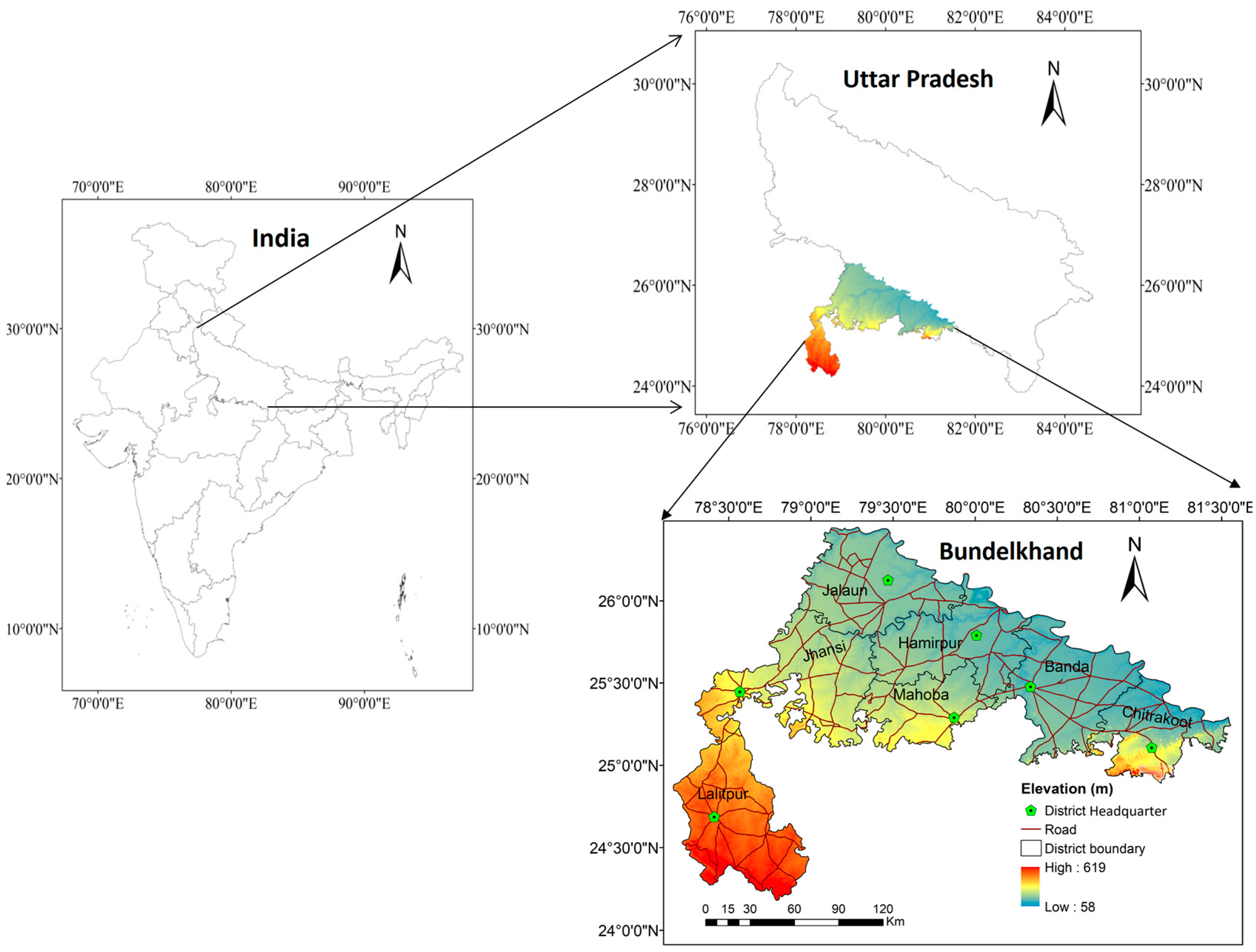
The Bundelkhand region (29,485.34 km²) was chosen as the study site, located below the Indo-Gangetic plain to the north and spread north-west of the undulating Vindhyan mountain range. The entire Bundelkhand region comes under the semi-arid zone and has four distinctive seasons, i.e., winter, summer, monsoon, and post-monsoon. The Bundelkhand region comprises the seven districts of Uttar Pradesh and six districts of Madhya Pradesh. The Uttar Pradesh region of Bundelkhand is the worst affected drought area, and it lies between latitudes 24°18′ and 26°45′N and longitudes 78°16′ and 81°56′E (Figure 1). The maximum altitude of this region does not exceed 619 m Mean Sea Level (MSL), with an overall slope from the southern to northeastern region. It is a gently sloping upland, distinguished by barren hilly terrain with sparse vegetation. Crops and barren land are the dominant land covers in the study area. It is a predominantly rural area with poverty and morbidity due to unemployment and polluted potable water. The major rivers flowing through this region are the Sindh, Betwa, Ken, Bagahin, Tons, Pahuj, Dhasan and Chambal, which constitute part of the Ganga river basin. The major soil type includes alluvial, medium black, and mixed red and black soils. Agriculture is a secondary occupation in Bundelkhand, as the majority of the area lies in wasteland due to recurrent drought events. The production in this area is primarily determined by water availability. Due to the scarcity of ground water resources, the main source of irrigation in the area is rainfall; consequently, most of the area cultivates Rabi crops. The majority of grown crops belong to the pulse category. Gram and wheat were the main Rabi crops, whereas jowar and bajra are grown during the Kharif season (July–October). A variety of coarse crops (millets) like mandwa, kodon, sawan, kakun and kutki are also dominantly grown in the area due to its productivity during short growing periods under dry conditions (http://www.bundelkhandinfo.org.in).

3. Materials and Methods

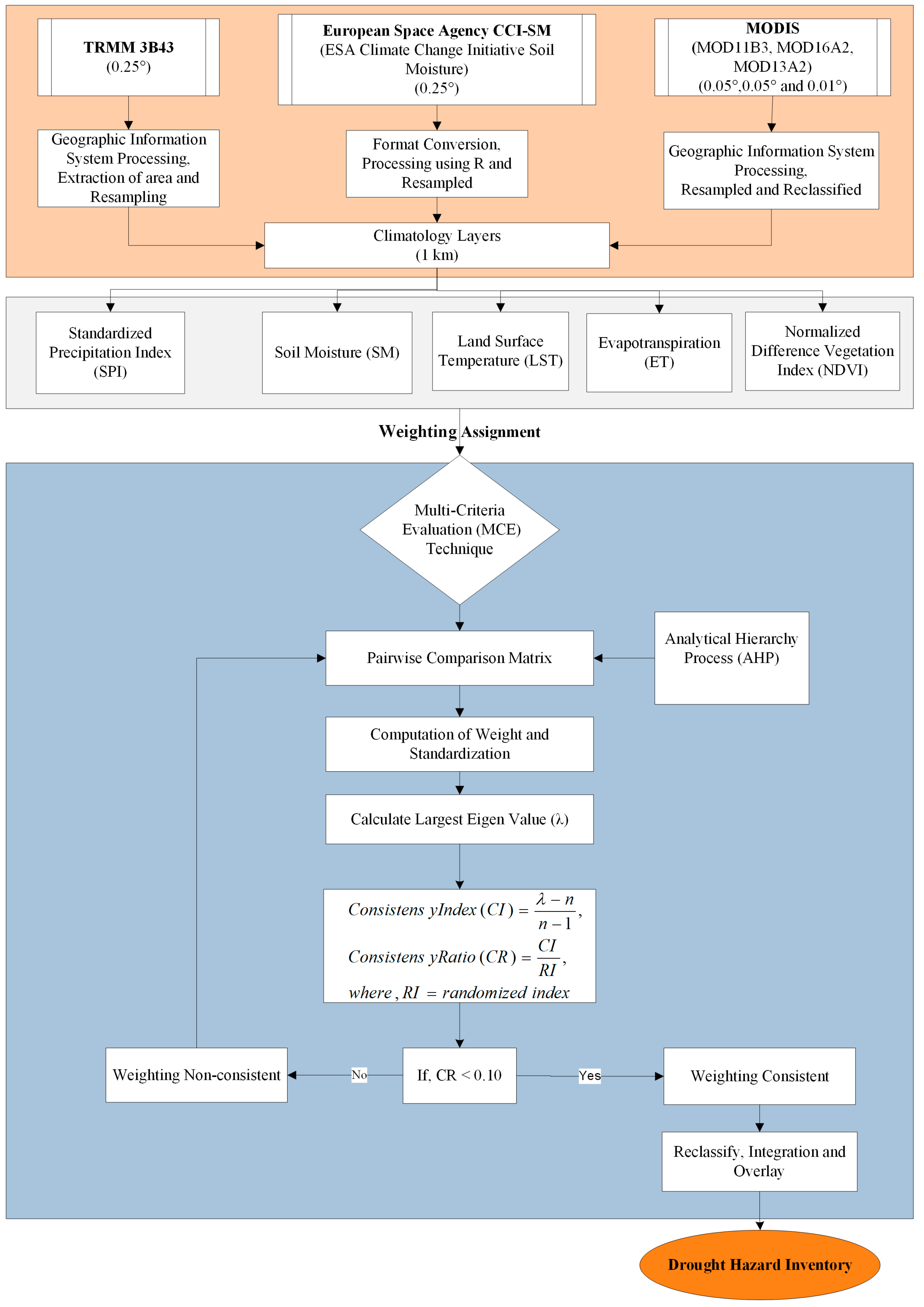
Rf, LST, SM, ET, and NDVI satellite datasets were taken for the development of DHI. These input thematic layers were prepared for the monsoon season (June- September: JJAS) for a 13 years period from 2002 to 2014 in the geospatial platform. For this, we first determined the priorities of the given alternatives (layers) by a pair wise comparison technique and then computed the weights by applying a decisive AHP technique. Following this, each layer was standardized, in order to be converted in a uniform scale ranging from 0 to 100. To avoid any spatial mismatch, the aforementioned thematic layers were resampled to a common grid size, i.e., 1 km in a common spatial reference frame and coordinate system Universal Transverse Mercator (UTM) zone 44 N. Finally, the weighted overlay analysis was performed for the integration and generation of the DHI map. The schematic diagram of this methodology is shown in Figure 2.

3.1. Data Acquisition and Preparation

3.1.1. The Tropical Rainfall Measuring Mission (TRMM) Rainfall Products

The dataset of the Tropical Rainfall Measuring Mission (TRMM) is used in this study for the seasonal rainfall climatology product development. TRMM 3B43 data are freely available from the NASA database (http://trmm.gsfc.nasa.gov/data_dir/data.html). The 3B43 algorithm provides the best estimate of the total monthly rainfall in a complete record from January 1998 to the present, with the continuation of the Global Precipitation Mission (GPM). The real-time precipitation information of TRMM is available in a 0.25° × 0.25° spatial and daily temporal resolution. In this study, the mean seasonal rainfall over thirteen years (2002–2014) was considered and averaged for a climatology layer preparation. The resulting raster layer was standardized to a convert factor map using a uniform scale ranging from 0 to 100. The resulting layer was then reclassified into four classes using an equal interval. The reclassified map is categorized from zone I (for the least rainfall) zone IV (for the highest rainfall in the study area).

3.1.2. The European Space Agency (ESA) Climate Change Initiative Soil Moisture (CCI-SM) Product

Climate Change Initiative Soil Moisture (CCI-SM) provides global long-term consistent soil moisture dataset. The Soil Moisture CCI project is a part of the ESA Programme on Global Monitoring of Essential Climate Variables (ECV), initiated in 2010. The project focuses on C-band scatterometers (ERS-1/2 scatterometer, METOP Advanced Scatterometers), multi-frequency radiometers (SMMR, SSM/I, TMI, AMSR-E, Windsat) as well as the Soil Moisture Ocean Salinity (SMOS) and Soil Moisture Active Passive (SMAP) mission (in phase 2), as these sensors are characterized by their high suitability for soil moisture retrieval and a long technological heritage. The data is available at 25 mm spatial and daily temporal resolutions (www.esa-soilmoisture-cci.org/). The volumetric soil moisture datasets are available in units of m³m⁻³. The data availability and quality have improved due to a day by day increase in satellite sensors, which has rapidly increased the number of studies using CCI-SM [29,30,31,32]. CCI-SM represents the moisture available in the soil from the surface to a depth of a few millimeters to centimeters from the soil surface. Three SM products are available through CCI-SM program viz., Active, Passive and Combined. We intended to use "Combined Product" for analyzing the soil moisture condition for the period of 2002 to 2014 in the study site; however, we observed that within the monsoon period the CCI-SM fluctuation is very low. Dorigo et al. [33] evaluated CCI-SM on a global scale and found a very close relationship between ground observed data and CCI-SM datasets. Chakravorty et al. [34] studied the sensitivity of CCI-SM over the Indian subcontinent and observed its better performance for seasonal and anomalous events. However, finding its close relevance with in-situ data, we used the obtained CCI-SM thematic layer as an effective input layer for the evaluation of DHI using AHP-based MCDM. The daily SM data were converted into long-term climatology of particular monsoon months by summing the valid SM observation for a particular month and dividing this sum by the day having valid SM observations. Then the study area shape was used to subset the layer in the R platform, before being resampled in a 1 km grid size with a UTM zone 44 N spatial reference.

3.1.3. Monthly MODIS LST, ET, and NDVI Data

The Moderate Resolution Imaging Spectroradiometer (MODIS) program, having sensors on two satellites (Terra and Aqua) provides images in 36 spectral bands between 0.405 and 14.385 μm. We took the LST (MOD11B3), ET (MOD16A2) and the monthly NDVI (MOD13A2) for our study. The former two products were obtained from the Land Processes Distributed Active Archive Center (LP DAAC; https:// lpdaac.usgs.gov/) database and later one from NASA Earth Observations (https://neo.sci.gsfc.nasa.gov/) free of cost. The MOD11B3 version 6 products provide a monthly LST with a 0.05° (5600 m) spatial resolution. The Global MOD13A2 NDVI images are produced from MODIS with a monthly temporal and 0.01° (1 km) spatial resolution. In addition, the global MODIS ET product (MOD16A2) with the temporal resolution of one month and spatial resolution of 0.05° was obtained from the University of Montana’s portal (http://files.ntsg.umt.edu/data/NTSG_Products/). These level-3 MODIS data were downloaded for the monsoon season (JJAS) for the derivation of the climatology.

3.1.4. Ground Water Record

To validate the DHI, the ground water level of the study period was assessed. We obtained ground water level data for the Bundelkhand UP region for the pre-monsoon (March, April, and May) and Monsoon (JJAS) periods for the thirteen years (2002–2014) from the website of the Central Ground Water Board (CGWB), Ministry of Water Resources, Govt. of India (http://cgwb.gov.in/GW-data-access.html). Ground water level/ piezometric head data are being monitored using dug wells and piezometers by the CGWB. 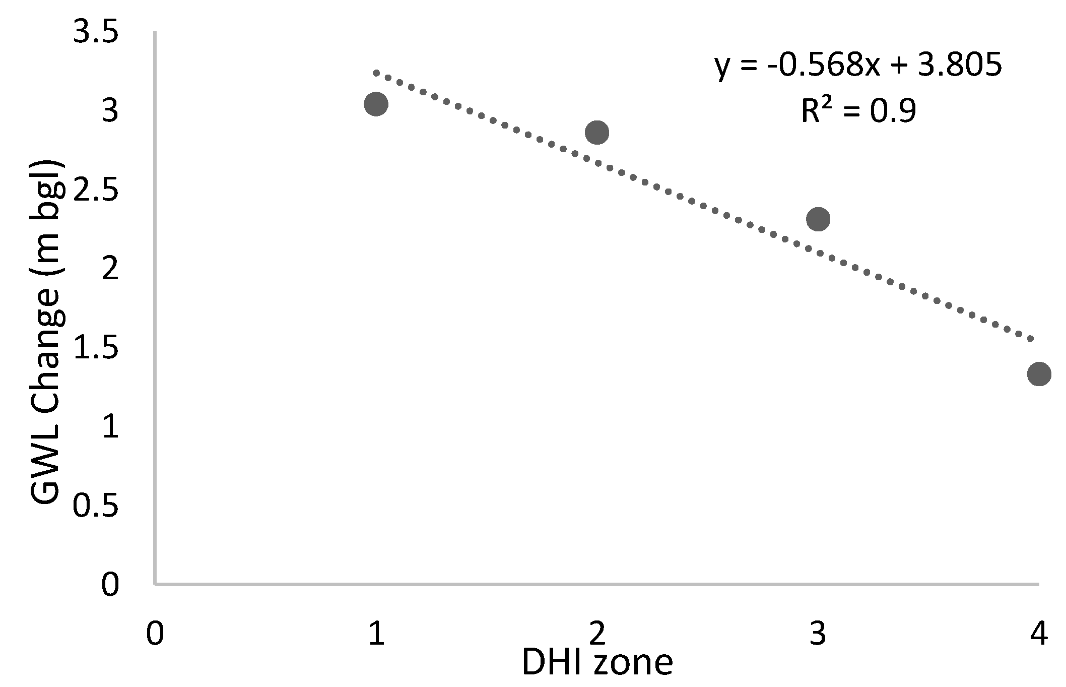The CGWB monitors the ground water level data four times a year with 22,339 ground water observation wells (both piezometer (6149) and dug wells (16,190) in India, excluding Mizoram, Sikkim, and Lakshadweep (http://cgwb.gov.in). We prepared the long-term climatology of the monsoon and pre-monsoon ground water level using 108 well points within the study area. The mean groundwater level fluctuation between monsoon and pre-monsoon was derived to validate the DHI, considering that a lower change in the ground water level could be the reason for a higher drought and vice-versa.

3.2. Multi-Criteria Decision Making (MCDM) Technique and Analytical Hierarchy Process (AHP)

MCDM is a decisive technique that evaluates a problem by sequencing a preference for multiple alternatives using several criteria that may have different units [35,36]. The technique of MCDM is used for weighting assignments for each layer. It is a widely used concept, which enables decision makers to build the most suitable choice among different criteria [19]. The main objective of the MCDM approach is to compare and rank alternatives as well as to evaluate their consequences based on established criteria. In the application of MCDM, Saaty and Vargas [37] proposed one such multi-criteria decision analysis that is the analytical hierarchy process (AHP). In the AHP, pairwise comparisons were made to generate a matrix for the selection of preferred elements in terms of their performance. The AHP thus significantly judged the participation of given criteria/alternatives for achieving particular goals by defining priorities to the factors [38]. Similarly, this technique is used to convert intangible qualitative criteria into tangible quantitative criteria. In the AHP, the rating is done on a scale of 1 to 9 as proposed by Saaty [39]. 1 represents the lowest contributing value, while 9 represents the highest, in increasing order of scale. The selection of the criteria and judgments are done based on the decision makers’ knowledge, experience and with reference to previous studies. As the user determines the judgments subjectively, logical consistency is required in the last level of the AHP analysis.

The weighting of each factor can be derived after a pairwise comparison by a linear algebra transformation. Furthermore, the Consistency Ratio (CR) is used for an estimation of the random probability of values obtained by a pairwise comparison matrix. CR is the division of consistency index (CI), i.e., maximum eigenvalue of the matrix and random inconsistency index (RI) [40]. Equations (2)–(4) show the mathematical expression of the MCDM-AHP technique. C = [C j, J = 1, 2, …, n] as the set of criteria. An evaluation matrix A (n _ n), in which each element a_ij (i, j = 1, 2, …, n) is the quotient of weights of the criteria, presented the result of a pair wise comparison matrix of n criteria as follows: as follows,

$$A=\left(\begin{array}{ccc}{a}_{11}& a_{12}\cdots & a_{1n}\\ a_{21}& a_{22}\cdots & a_{2n}\\ a_{n1}& a_{n2}\cdots & a_{nn}\end{array}\right),a_{ij}=1,a_{ij}=1/a_{ij},a_{ij}\ne 0$$

(1)

First, we estimated the biggest eigenvalue of the pairwise comparison matrix, i.e., λ_max using the following formula:

$${\lambda }_{\max }=\frac{1}{n}{\displaystyle {\sum }_{i=1}^n\frac{x_i}{c_i}}$$

(2)

where n is the number of criteria; and c_i and x_i are the relative degree of importance (weight) and approximation to the eigenvector of the ith objective. Finally, the relative weight is derived by the right eigenvector (w) with respect to the biggest eigenvalue (λ_max), as shown in the following Equation (3):

$$A_w={\lambda }_{\max }w$$

(3)

In the last step of the AHP, we calculated an approximation to the consistency index (CI) that measured the inconsistency of pairwise comparisons (zero value shows the perfect consistency). The consistency index can be measured using reciprocal matrices. In reciprocal matrices, the maximum eigenvalue (λ_max) should be greater than or equal to the number of rows and column (n). The consistency index CI is given by Equation (4):

$$ConsistencyIndex(CI)=\frac{{\lambda }_{\max }-n}{n-1}$$

(4)

Finally, the measurement of coherence of the pairwise comparisons was calculated in terms of the Consistency Ratio (Equation (5)). The RI value for the number of criteria n is given in

Table 1. Random Inconsistency Index (RI) values with different n [39].

n	1	2	3	4	5	6	7	8	9	10
RI	0.00	0.00	0.58	0.90	1.12	1.24	1.32	1.41	1.45	1.49

.

$$ConsistencyRatio(CR)=\frac{CI}{RI}$$

(5)

These parameters are useful for precise and effective decision-making and consequently for the weighted analysis. The CR index determined the credibility of the AHP evaluations. The threshold of the CR is ≤10% (≤0.10). Thus, if the CR is equal to or less than 0.10, the consistency is acceptable, but if the CR is greater than the former value then, because of an inconsistent treatment of a particular factor rating, the subjective value judgment is reevaluated. This consistency measurement is very important in terms of the evaluation of the credibility of the consistency of the hierarchy and decision makers.

3.3. AHP-GIS Implementation Strategy for DHI

The criteria used in this study were effectively contributing to the onset of drought on a priority basis. The available literature was useful for assigning a rate to the selected parameters [4,41,42,43,44]. The factor with a higher weight value denotes a higher priority/ impact in comparison to other factors within the study [19]. In this case, the most important layer was considered to be the Rainfall (Rf); that is because its deficiency is the prime factor that causes drought [42,44]. A lack of water (rainfall) availability significantly reduces the moisture content in soil, enhances the land surface temperature and consequently increases the ET rate, and it contributes directly in deriving drought for those given moderate preferences. Such conditions result in the deterioration of vegetation health, and they are given the least preference in the analysis [4,45].

Owing to the different scale and units of the input data, we normalized or standardized all the layers before processing them with the minimum and maximum (0 to 100) using the following Equation (6):

$$S_i=\frac{(X_i-X_{\min })}{(X_{\max }-X_{\min })}\times (S_{\max }-S_{\min })+S_{\min }$$

(6)

where, S_i is the standardized output; X_i, X_min and X_max are the input data, minimum and maximum cell values respectively; and S_max = 100 and S_min = 0 are the maximum and minimum standardized scale values respectively. Following this, all the standardized output layers were used in the weight assignment using a pairwise comparison matrix in the context of the decision-making AHP approach. In this step, each criterion was assigned a weight with respect to its significant contribution to drought hazard. The rating and weight assigned to each criterion are shown in

Table 2. Pair comparison matrix of thematic layers. Where Rf, SM, LST, ET and NDVI are rainfall, soil moisture, land surface temperature, evapotranspiration and normalized difference vegetation index respectively.

	Rf	SM	LST	ET	NDVI	Normalized Weight
Rf	1	2	4	5	6	44.5
SM	1/2	1	3	2	4	25.2
LST	1/4	1/3	1	3	4	15.8
ET	1/5	1/2	1/3	1	3	9.5
NDVI	1/6	1/4	1/4	1/3	1	5.0
Consistency Ratio = 0.065

. The consistency for the weighting assignment was then checked in terms of the CI and CR values after the MCDM-AHP analysis.

The CI was computed using the principal eigenvalue of this pairwise comparison, i.e., 5.295. The CI was obtained as Equation (7):

$$CI=(5.29-n)/(n-1)=0.074$$

(7)

here, n = 5 is the number of input variables.

The CR value is then computed as; CR = CI/RI = 0.065, where RI is obtained from Table 1, as 1.12. The CR value obtained is under the threshold value of 0.1 and hence showed the consistent pairwise judgment, implying acceptable determined weights. After obtaining a reliable CR value (<0.1), we proceeded, for the weighted overlay, to derive DHI. With the consistent weights obtained through a pairwise comparison matrix, the layers were weighted overlaid. The weighted overlay can be mathematically expressed as follows:

$$DHI=R{f}_{wt}R{f}_{sc}+S{M}_{wt}S{M}_{sc}+LS{T}_{wt}LS{T}_{sc}+E{T}_{wt}E{T}_{sc}+NDV{I}_{wt}NDV{I}_{sc}$$

(8)

where X_wt and X_SC are the normalized weights of the criterion and the standardized criterion raster maps respectively. The obtained DHI map denoted the magnitude of drought hazard within the study area and can be grouped into four categories: low, moderate, high and very high hazard zones.

4. Results

4.1. Rainfall Distribution

The TRMM 3B43 datasets derived a seasonal rainfall anomaly (percentage) from 2002–2014 for the Bundelkhand-UP region, as shown in Figure 3, indicating that the departure from the long-term average value allowed for more precise observations than the actual rainfall; it provided a frame of reference for easier analysis. A positive and negative anomaly indicates that the rainfall was above or below the annual average rainfall. The drought condition based on the rainfall intensity can be best observed on a yearly basis via the graphical representation of its anomaly. It has been observed that five drought events occurred from 2002 to 2014 in the study area (Figure 3). With reference to past studies, severe droughts were identified in 2002 and 2006; and extreme droughts were observed in 2007, 2009 and 2014, with an anomaly of −19 to −31 [46,47].

To understand the rainfall distribution in the monsoon season (JJAS), an average time series graph was plotted for the period of 2002–2014 (Figure 4a). The highest rainfall was observed in the month of July (30.44 to 216.18 mm) followed by August and June (between 7.5 to 135 mm), and then September (10.5 to 94 mm). Furthermore, we used the box-whisker plot to denote the distribution and Skewness, divided into lower quartile, median (middle line) and upper quartiles values, with the whiskers extending at each end showing the range of rainfall (Figure 4b). The observed plot exhibits a normal distribution curve, gradually increasing from June to July and then decreasing to September. The rainfall ranges in June were observed to range from 7.5 to 135 mm, reaching 167 in the year 2002. Similarly, in July, August, and September, the rainfall ranges were observed in a range from 30.5 to 216 mm, 63.6 to 159 mm and 10.5 to 94 mm, respectively. In September, the rainfall was 203 and 213 mm in the years 2010 and 2014, respectively, representing the outliers.

The long-term rainfall climatology varied between 590 mm and 965 mm, clearly showing that the lower monsoonal rainfall occurring in the northern part: Jalaun, Jhansi, Hamirpur and some parts of Banda; the higher monsoonal rainfall occurred in the southern part: Chitrakoot, Lalitpur, and some parts of Banda in the study area (Figure 5a).

4.2. Variations in Land Surface Fluxes

We have derived the soil moisture climatology during 2002–2014 (13-year average; unit m³m⁻³) for the monsoon season (Figure 5b). The spatial pattern of soil moisture climatology showed marked variations across the landscape within the monsoon season. The soil moisture ranged from 0.18 m³m⁻³ to 0.29 m³m⁻³, indicating dry to moderately wet regions, respectively. The spatial pattern of the map illustrates a higher soil moisture content in the southern part due to a high drainage density, reservoirs and forest cover. (Lalitpur, Chitrakoot and some southern part of Jhansi, Mahoba and Banda district) compared to the central northern region (Jalaun, Hamirpur and northern part of Jhansi, Mahoba and Banda district).

For the study area, the observed evapotranspiration ranges from 645 mm per season to 983 mm per season (Figure 5c). The ET climatology map for the monsoon season showed a strong variability with marked differences between the central northern plain regions, and southwest and southeast regions in the area. It could be used to denote the combined influence of the temperature, elevation gradient, and water storage. Within the area, the lowest ET was observed in the central northern part, owing to low rainfall and soil moisture conditions (Figure 5a,b). Whereas, the higher ET in the southwest and southeast region could be due to higher rainfall, soil moisture, as well as the reservoir and forest covers.

Besides rainfall, evapotranspiration and soil moisture, another significant factor for drought monitoring is the LST. Figure 5d shows that the climatology of the seasonal mean land surface temperature for the monsoon season ranged from 29 °C to 40 °C, with a mean of 37 °C. We observed a chaotic pattern with a high temperature in the central northern part. A higher LST was observed in the central and northern parts, and a lower LST in the southwest (Lalitpur) and moderate southeast region (Chitrakoot).

4.3. Normalized Difference Vegetation Index (NDVI)

The NDVI is one of the effective indicators of drought condition expressed via vegetation health. A multi-year (2002–2014) average NDVI map is shown in Figure 5e. The NDVI climatology showed moderate NDVI values, ranging from +0.27 to +0.62, representing sparse vegetation such as senescing crops or grassland (Figure 5e). Higher NDVI values were observed mostly in the Chitrakoot and Lalitpur districts, which could be attributed to the presence of continuous forest covers, as well as cropland around the reservoirs. Higher NDVI values were also observed in some parts of the Mahoba and Jhansi districts; meanwhile, lower NDVIs were observed in the rest of the study area. The NDVI climatology exhibited a similar pattern, enabling an unbiased comparison; it followed the soil moisture, evapotranspiration, and rainfall distribution.

4.4. Multi-criteria Decision Making (MCDM) Technique and Drought Hazard Inventory (DHI)

A DHI map was generated by a weighted overlay analysis, applying the normalized weight obtained by a pairwise comparison matrix of the AHP technique with standardized criterion maps (Figure 6). The DHI is a combination of the major factor causes, and it exhibits drought hazard; the decisive techniques and experts’ judgments made it more effective and versatile than other drought indices. The rating and weights obtained by the MCDM-AHP analysis were given in Table 2. The highest standardized weight (44.5%) was given to rainfall, followed by SM (25.2%), LST (15.8%), evapotranspiration (9.5%) and NDVI (5.0%), with a CR value of 0.065. About 38.05% and 27.54% of the total area was estimated to be high and extreme (very high) drought-prone zones, respectively. Meanwhile, about 15.83% and 18.58% of the total area were found to be in the lowest and moderate drought hazard category (

Table 3. Percent of total area in each Drought Hazard Inventory (DHI) class and its comparison with the ground water level.

Zone	DHI Category	Percent Area	Number of Ground Water Data Points	Mean Ground Water Level (m bgl)
				Pre-monsoon	Monsoon	Change
I	Low	15.83	8	6.65	3.61	3.04
II	Moderate	18.58	27	9.89	7.03	2.86
III	High	38.05	42	8.99	6.68	2.31
IV	Very high	27.54	31	10.92	9.59	1.33
			108	9.60	7.38	2.22

, Figure 6).

4.5. Validation of Results Using the Ground Water Level Change

The obtained result was validated with the ground water level fluctuation during the period under investigation. The monsoon and pre-monsoon ground water level of 108 wells in this region was averaged over thirteen years. The average depth of the ground water table was classified into four categories (Table 3). We observed a lower ground water level in the pre-monsoon compared to the monsoon; the average ground water in the pre-monsoon varied between 6.65 m bgl (meters below ground level) and 10.92 m bgl; it varied between 3.61 and 9.49 m bgl in the monsoon season. We observed significant differences in water recharges in different districts (Figure 7). The average change in the ground water level varied between −0.32 and 8.28 m bgl during the study period. Using the inverse distance interpolation technique, we created the surface raster indicating the spatial change in the ground water level. The spatial average change in the ground water level in each DHI zone was extracted using the zonal statistics tool.

The spatial average difference in the ground water level among the DHI zones varied between 3.04 m bgl and 1.33 m bgl (Figure 8). The highest ground water recharge was seen as 3.04 m bgl in the lowest DHI category, followed by 2.86 m bgl, 2.31 m bgl, and 1.33 m bgl in the moderate, high and very high DHI categories, respectively. Again, the spatial map of the ground water change is shown in Figure 7, exhibiting higher ground water recharges in Chitrakoot, Lalitpur, moderate ground water recharges in Banda and part of Hamirpur, and lower ground water recharges in Mahoba, Jhansi, and Jalaun, which is in agreement with the DHI developed in this study.

The coefficient of determination (R² = 0.9) between the average ground water recharge and DHI categories exhibited a higher ground water recharge in the area with low chances of drought hazard, and decreases with the increase of drought hazard severity; this, therefore, validated the robustness and significance of the output. The spatially explicit map provides a rigorous finding of drought-prone areas, which can be used for the planning and construction of effective drought mitigation practices.

5. Discussion

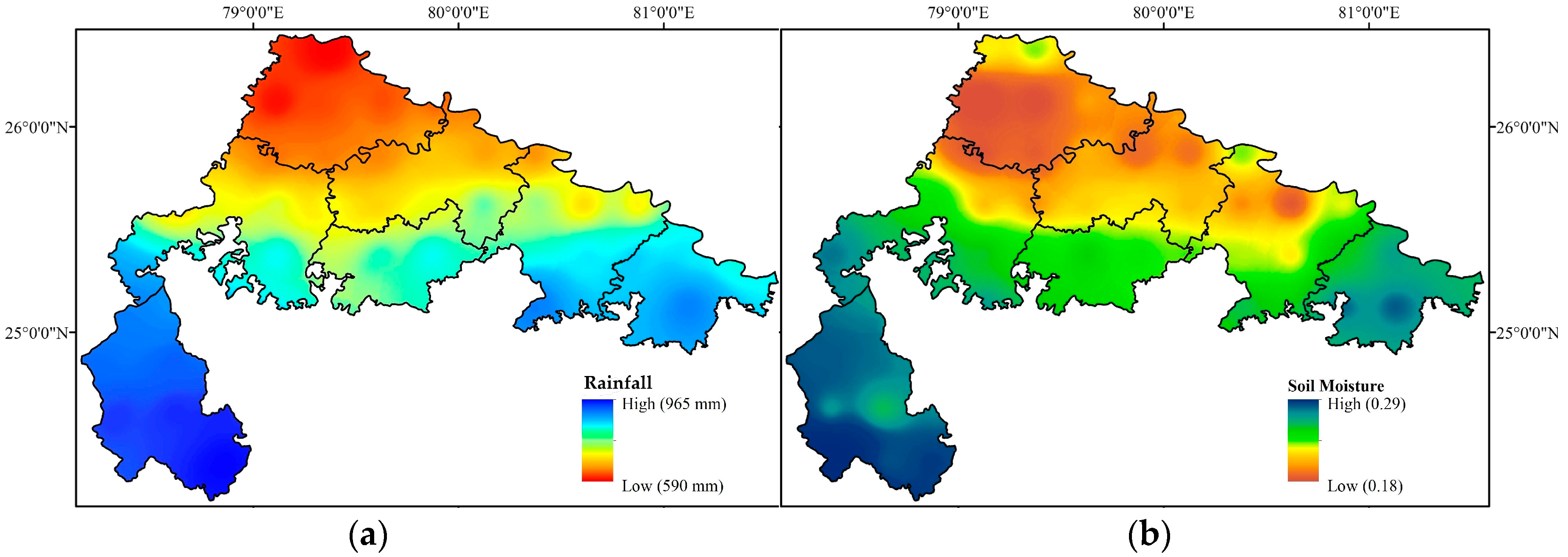
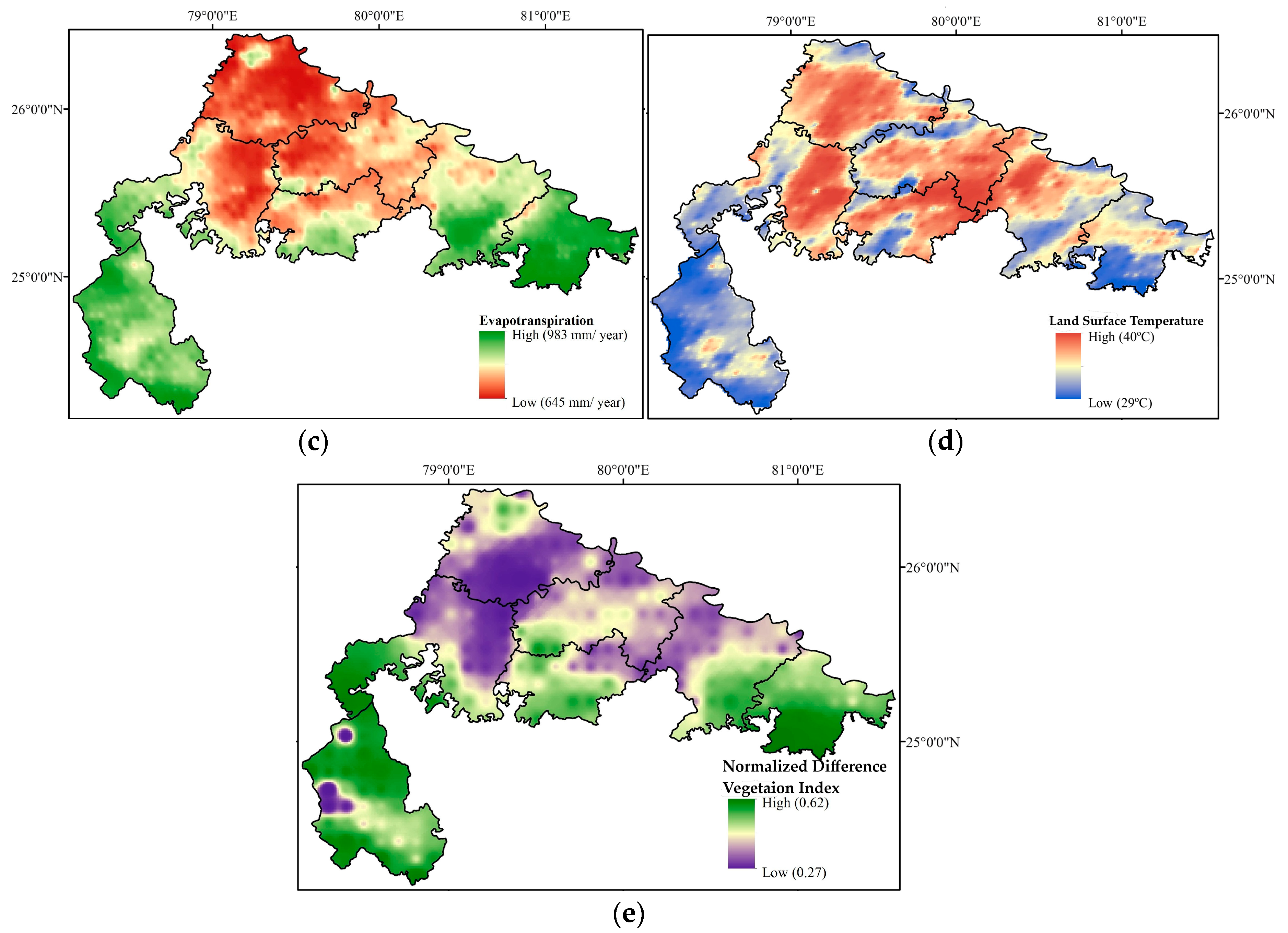
The results obtained via different variables accentuate the annual dry season and therefore drought conditions on the study site. The districts located in the central northern part of the study area, i.e., Jalaun, Hamirpur, Jhansi, and Banda, were estimated as being the most vulnerable regions for drought, as a result of the combined influence of the lower rainfall, soil moisture, NDVI, and higher LST and ET [7]. The increase in temperatures leads to decreases in soil moisture and high ET. Minimum ET rates are normally found during the winter season and maximum ET rates occur usually in the summer season of the year. Apart from the temperature, the ET depends on the availability of soil moisture and ground water storage as well as the vegetation condition. Meanwhile, the districts located in the southern part, i.e., Chitrakoot and Lalitpur, were found less prone to drought as a result of higher rainfall, SM, vegetation density, lower temperature, high number reservoirs and forest cover in the area [48]. Contrary to the normal conditions, the ET rates that were found were higher in this region, but this does not show drought conditions as this region contains high forest cover and reservoir density when compared to the other regions. Therefore, in the weighted overlay, the areas with higher rainfall, SM, and NDVI, as well as lower LST and ET, were used as an indicator for less severity to drought events and vice-versa, where the weighted overlay integrated the combined effect of individual factors into a single index map.

The three basic steps are applied in this study for assessing drought hazard. First, the determination of effective factors or variables causing drought hazard; second, the standardization of each factor, and third, the application of the GIS-aided AHP technique for finding the drought hazard zone. One of the main advantages of the selected AHP methods is that it evaluates the comparative significance of all input thematic indicators based on the assessment of weights by pairwise comparison judgments in a hierarchical manner [49,50,51]. Rf, SM, NDVI, LST, and ET, the main variables for drought assessment, were used in this study to estimate their cumulative impact on the selected region. To achieve a single index map for mapping drought-prone areas, we opted for the MCDM technique; this can be a more pragmatic technique for implementing drought hazard mitigation. The validation process that exhibited a higher ground water recharge in the lower drought hazard zone and vice-versa supports the results obtained in this study.

The results obtained by our study also illustrated that the AHP might solve a complex problem in the MCDM environment, based on expert knowledge and judgment, in a flexible, sequence-wise and transparent way. Furthermore, this approach for drought hazard assessments seems inexpensive, convenient and interactive process that uses expert decisions for continued improvement. The use of geospatial data, Earth observations, and analyses in a GIS environment enable better evaluation of the spatially explicit data, a quick modification or data update, and a faster repetition of the process. The drought-prone zone under the study area revealed the importance of canals and reservoirs, representing how necessary it is to include them in drought mitigation and management plans. Moreover, the resulting maps may assist decision makers, as well as governmental and non-governmental organizations, for the better management of drought events and for applying mitigation measures that ensure food security, especially in the era of climate change. Moreover, the influence of the input layers may vary with the number of input layers, which is again highly dependent on the study area. However, the opted methodology, simplistic data integration approach, and reliability of the outcome proved its importance for quick and first-hand assessments of repetitive drought conditions in a region. Moreover, the water harvesting structures can be constructed extensively in the drought-prone regions for both the ground water recharge and the maintenance of soil moisture in the area. Further research will continue to focus on drought risk in order to characterize the impact of droughts on agricultural productivity and livelihood.

6. Conclusions

In a recurrent drought-affected area, the identification of drought a hazard zone is a prerequisite for planning purposes. This study was carried out in the Bundelkhand region, primarily with the objective of developing a methodology that identifies drought hazard-prone zones using the remote sensing and GIS-aided multi-criteria evaluation technique. For the preparation and standardization of input layers (factors and constraints) for the DHI, an integrated approach based on remote sensing and GIS were taken into consideration through the MCDM approach. The results depicted that around 65.59% of the total study area of the central northern part comes under a zone vulnerable to drought, with different magnitudes (extreme and high); meanwhile, about 34.41% of the southern part is found to be the least vulnerable (moderate and low) to drought hazard. Moreover, the study focuses on the exploration of the importance of space-born datasets to characterize the drought phenomenon in the Bundelkhand region, to provide more insights for improved decision-making and planning. This is significant for decision-makers as it gives an itinerary for required drought preparedness measures. The methodology used in this study represents a prototype for assessing drought on a large scale as well as in remote areas where ground-measured data are limited. The prototype attempted in this study can be used to solve the large-scale drought monitoring of vulnerable areas. Therefore, we can conclude that the MCDM technique using space-born datasets is very effective technique for delineation of drought hazard areas.