A Fine Velocity and Strain Rate Field of Present-Day Crustal Motion of the Northeastern Tibetan Plateau Inverted Jointly by InSAR and GPS

Abstract

Interferometric synthetic aperture radar (InSAR) data from 6 Envisat ASAR descending tracks; spanning the 2003–2010 period; was used to measure interseismic strain accumulation across the Northeastern Tibetan Plateau. Mean line-of-sight (LOS) ratemaps are computed by stacking atmospheric-corrected and orbital-corrected interferograms. The ratemaps from one track with different atmospheric-corrected results or two parallel; partially overlapping tracks; show a consistent pattern of left-lateral motion across the fault; which demonstrates the MERIS and ECMWF atmospheric correction works satisfactorily for small stain measurement of this region; even with a limited number of interferograms. By combining the measurements of InSAR and GPS; a fine crustal deformation velocity and strain rate field was estimated on discrete points with irregular density depending on the fault location; which revealed that the present-day slip rate on the Haiyuan fault system varies little from west to east. A change (2–3 mm/year) in line-of-sight (LOS) deformation rate across the fault is observed from the Jinqianghe segment to its eastern end. Inversion from the cross-fault InSAR profiles gave a shallow locking depth of 3–6 km on the main rupture of the 1920 earthquake. We therefore infer that the middle-lower part of the seismogenic layer on the 1920 rupture is not yet fully locked since the 1920 large earthquake. Benefit from high spatial resolution InSAR data; a low strain accumulation zone with high strain rates on its two ends was detected; which corresponds to the creeping segment; i.e., the Laohushan fault segment. Contrary to the previous knowledge of squeezing structure; an abnormal tension zone is disclosed from the direction map of principal stress; which is consistent with the recent geological study. The distribution of principal stress also showed that the expanding frontier of the northeastern plateau has crossed the Liupan Shan fault zone; even arrived at the northeast area of the Xiaoguan Shan. This result agrees with the deep seismic reflection profile.

1. Introduction

Surface velocity and strain fields provide an important constraint on geodynamic models of tectonic deformation as well as in the assessment of earthquake hazard [1]. Such velocity fields may be determined using geodetic measurements such as GPS, but GPS observations are too sparse to describe deformation spatial variations in the near-fault area. Increasing Synthetic Aperture Radar (SAR) coverage allows SAR interferometry (InSAR) to be used as a complementary or alternative means of measuring deformation of the Earth’s surface. InSAR has been successfully used to determine coseismic deformation of many earthquakes (e.g., the 2003 Bam earthquake [2], 2011 Yushu earthquake [3], and 2015 Nepal earthquakes [4]) and post-seismic deformation (e.g., Atzori et al. 2008 [5] and Gonzalez-Ortega et al. 2014 [6]), as well as deformation related to earthquake swarms (e.g., Kyriakopoulos et al. 2013 [7] and Wicks et al. 2011 [8]). In recent years, InSAR has begun to perform well in measuring the rate and distribution of interseismic strain accumulation with the increasing satellite data volume (e.g., in Northwestern Tibet [9,10], the San Andreas fault system [11,12,13], the Anatolian Fault system [1,14,15], and the Haiyuan fault system in the northeastern margin of the Tibetan Plateau [16,17,18,19]). Satellite InSAR data provide us a chance to give an insight into the near-fault crustal displacement caused by the fault motion, particularly for the shallow aseismic fault slip. It has provided important information on imaging the spatial variation of interseismic coupling on the fault plane in the upper crust. As well as benefitting from its ability to characterize both the long- and short-wavelength deformation with a high accuracy, InSAR also provides new knowledge for improving our understanding the processes of crustal deformation caused by interaction of faults or blocks in some fault transferring zones and the block boundary belts.

In this paper, we focus on the northeastern margin of the Tibet Plateau, where the crustal shortening and lateral extrusion caused by the northeastward growth of the Tibet Plateau is accommodated by the left-lateral strike-slip Haiyuan fault and a series of arcuate structures in its north, and the thrusting Liupan Shan fault and a few folds and thrust faults in its east (Figure 1). Two large earthquakes occurred on the Haiyuan fault system in the last century. One (Mw > 8.0) with a 220 km long surface rupture occurred on the eastern part of the Haiyuan fault in 1920, resulting in 220,000 deaths [20]. The other one is the 1927 Mw 8.0 Gulang earthquake ruptured south-dipping thrusts situated at the south-eastern end of the Qilian Shan [21]. Between these two ruptured segments, a seismic gap with the 260 km length is identified as the Tianzhu gap with a high seismic potential [17,21]. Here, we combined the InSAR and GPS to give refined estimates of the amplitude and distribution of elastic strain accumulation on those boundary faults with a high spatial resolution. We show how deformation is distributed locally along the faults in this region, what their current strain accumulation rate is. Finally, we discussed the present-day fault kinematic behavior of the 1920 rupture, and the tectonic response of the Tibet–Ordos transition zone to the plateau expansion.

2. Tectonic Setting and Data Used

2.1. Tectonic Setting

In the northeastern margin of the Tibetan Plateau, the Haiyuan fault system is a major active tectonic feature, connecting the seismically active Qilian Shan in the west and the tectonically active Liupan Shan in the east, the latter abutting the relatively stable Ordos block (Figure 1). It is dominated by left-lateral strike slip faulting, which probably began in the late Pliocene or early Pleistocene, followed by late-stage folding and thrust faulting [23]. At its eastern end, left lateral slip on the N65°W striking Haiyuan fault zone is transferred into shortening on the generally north trending structures in the Liupan Shan. Three arcuate zones of both strike-slip and thrust faults with associated ramp anticlines, lie about 40–170 km north and northeast of the Haiyuan fault zone. From south to north, the individual structures that comprise this arcuate system are the Tianjin Shan-Mibo Shan, Yanton Shan, and Niushou Shan-Daluo Shan fault zones. Tectonic activity within these areas is generally mild in comparison with that in the Haiyuan structural zone [24].

The Holocene slip rate of the Haiyuan fault system, determined by measuring the offsets and ages of morphological markers, seems to vary from west to east. The left-lateral strike-slip rates in the west have been estimated as 19 ± 5 mm/year on the Lenglongling fault segment, and 12 ± 4 mm/year on the Laohu Shan fault further east [25,26]. However, He et al. [27,28] and Zheng et al. [29] suggest much slower slip rates of 4–5 mm/year on the Lenglongling fault and 4.4 ± 0.4 mm/year on the Laohu Shan fault. The Holocene slip rate estimates along the length of the 1920 rupture (including the Xihuan-Nanhua segment) in the east are 8 ± 2 mm/year [20] and 4.5 ± 2 mm/year [30], which are consistent with an average Quaternary slip rate of 5–10 mm/year [22]. The rates of deformation in the Tianjing Shan and Mibo Shan are about 1.5–2.7 mm/year, notably less than that in the south [24]. GPS profiles across the Qilian-Haiyuan fault show that the left-lateral strike-slip rates and shortening rates from the west to the east, are 4.0 ± 1.0 mm/year and 5.6 ± 1.5 mm/year along the Lenglongling segment, 3.6 ± 1.4 mm/year and 2.3 ± 1.2 mm/year along the Maomao Shan and Laohu Shan segment, and 4.2 ± 1.5 mm/year and 2.6 ± 1.5 mm/year along the 1920 rupture respectively [29]. InSAR results from ERS and Envisat ASAR data give apparent slip rates of 4.2–8 mm/year [16] and 5.3 ± 1.0 mm/year [17] near the junction between the 1920 rupture and Tianzhu gap (the Maomao Shan–Laohu Shan segment). Additionally, they highlight a strong strain concentration in the Laohu Shan fault zone and suggest the presence of creep at shallow depths. Furthermore, the smoothed InSAR time series reveals that the creeping rate on the Laohu Shan segment accelerated in 2007 [18].

2.2. Data

We collected the Envisat SAR stripmap images for 6 descending tracks, which cover the most part of the northeastern margin of the Tibetan Plateau (Figure 1). Interferometric data for each track spans the 2003–2010 period with 30 more acquisitions except for the track 247 (12 acquisitions). Interferograms with baselines of less than 200 m were produced for each track by using JPL/Caltech ROI_PAC software. A filled 3 arc sec (90 m) resolution Shuttle Radar Topography Mission (SRTM) digital elevation model (DEM) [31] was used to remove the topographic contribution to the interferometric phase changes. As we are only interested in long-wavelength features, the data were multilooked, reducing the sampling interval to ~320 m in order to improve coherence and retain the tectonic signal near the fault. The coherence threshold of 0.15 was used to mask out the decoherenced area for each interferograms. Then interferograms were unwrapped using the branch-cut method [32]. The resulting unwrapped interferograms will be selected to construct a chain for stacking in the InSAR ratemap estimation (Section 3.1). GPS data we used is from Gan et al. [22], which is with respect to the Eurasia-fixed Reference Frame.

3. Method

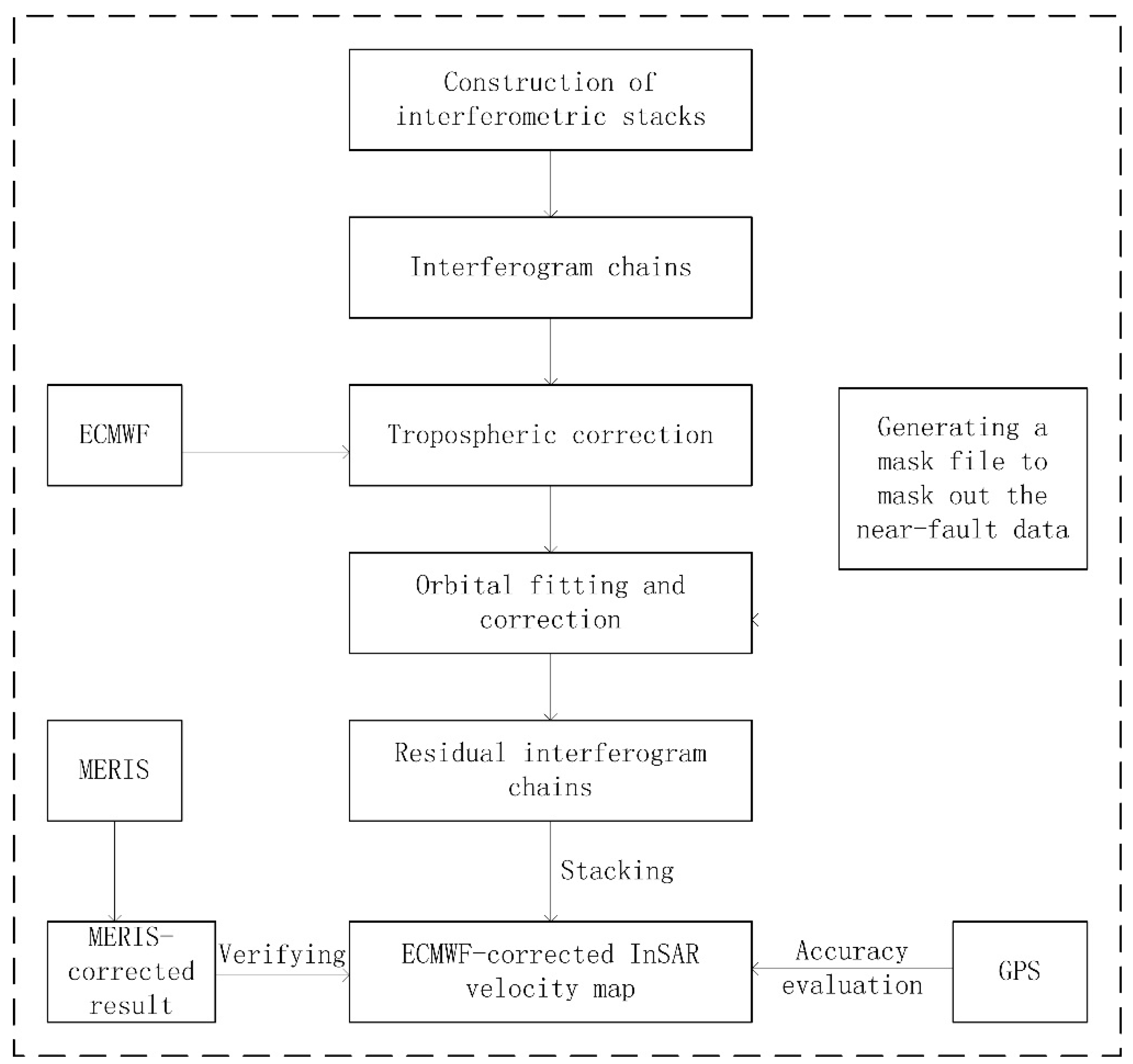
3.1. Stacking InSAR with Atmospheric-Corrected Interferograms

The detection of slow interseismic motion using InSAR requires a combination of multiple radar images over an extended time period to reduce the uncorrelated atmospheric effects and improve the signal-to-noise ratio. The total tropospheric delay is often divided into a stratified delay and a turbulent delay for InSAR applications [33]. Due to the high variability of atmospheric turbulence, the spatial pattern of the turbulent delay is mostly random on each acquisition date and can be removed efficiently by stacking interferograms [34] or through InSAR time series analysis [35]. Variations in atmospheric stratification have a first order effect, with a single path LOS delay reaching ∼10 cm/km in some areas [36]. Furthermore, unlike turbulent effects, stratified delays are not random in time but represent seasonal fluctuations and are therefore difficult to remove by stacking or temporal smoothing compared to turbulence, even when working with a large InSAR dataset. When we retrieve subtle ground displacements (e.g., millimeters per year on the Haiyuan fault), it is necessary to correct interferograms for the stratified tropospheric signals.

Given strong coupling between the linear orbital ramp, long-wavelength component of atmospheric error and long-wavelength tectonic deformation, external independent atmospheric data (ECMWF and MERIS) were used to correct the stratified tropospheric signals firstly, which is verified to be useful for correcting InSAR atmospheric effect [14,37]. Then a linear orbital trend was fitted and removed from the atmospheric-corrected interferograms, using only phase measurements 30 km or further from the fault in the north to avoid the effect of the near-fault gradient in ground deformation. After the atmospheric and orbital corrections, the residual interferograms from independent chains of small-baseline dataset (Figure S1) were stacked with a total timespan to create a ratemap. Only those pixels which are coherent in all interferograms were averaged with equal weight. The flowchart for retrieving an InSAR ratemap is showed in Figure 2.

3.2. Velocity and Strain-Rate Field Inversion from InSAR and GPS

A variety of algorithms have been developed to invert geodetic data for strains. The traditional subnetwork methods (e.g., [38,39]) usually generate discontinuities of the strain estimates at the subnetwork boundaries. The geostatistical methods can tackle the discontinuity problem. However, they assume that the deformation field is isotropic and homogeneous, and the accuracy and reliability often depends on the spatial distribution of the data (e.g., [1,40,41,42,43]). The physics-based models were developed to estimate the elastic and inelastic strain fields from geodetic data (e.g., [44,45]). Shen et al. [46,47,48] developed a series of algorithms to model strains with reasonable weighting and smoothing function optimally determined from observation data, which works well with unevenly distributed data, and can deal with the nonelastic strain accumulation caused by fault creeping in the upper crust. The surface deformation field caused by the strike-slip Haiyuan fault system, is not homogeneous and isotropic, and would changes cross the fault boundary. Previous InSAR results showed a creeping segment (the Laohu Shan segment) on the Haiyuan fault [17], thus the method in Shen et al. [48] was used in our study. We realized Shen’s method in a spherical coordinate system due to our big study area (500 × 500 km). Considering the high spatial coverage of InSAR velocity map, an irregular grid that discretized the study area based on the location of fault, is used in InSAR and GPS inversion, which allow us capture the strain variations near the fault.

For each node of the grid, its unknown vector can be related to the 3D velocity of its surrounding GPS observations by the following model:

$$u_{GPS}=A_{GPS}l,$$

(1)

where, $u_{GPS}$ is the vector of GPS observation, $l$ is the unknown vector of the displacement, strain, and rotation on each node of the grid, and $A_{GPS}$ is the design matrix. This observation equation can be expanded as:

$$\left(\begin{array}{l}{u}_{\varphi }\\ u_{\theta }\\ u_r\end{array}\right)=\left(\begin{array}{c}-\cos {\theta }_0\Delta \varphi \\ 1\\ \Delta \theta \end{array}\begin{array}{c}1\\ \cos {\theta }_0\Delta \varphi \\ \sin {\theta }_0\Delta \varphi \end{array}\begin{array}{c}-\sin {\theta }_0\Delta \varphi \\ -\Delta \theta \\ 1\end{array}\begin{array}{c}{r}_0\sin {\theta }_0\Delta \varphi \\ 0\\ 0\end{array}\begin{array}{c}{r}_0\Delta \theta \\ r_0\sin {\theta }_0\Delta \varphi \\ 0\end{array}\begin{array}{c}0\\ r_0\Delta \theta \\ 0\end{array}\begin{array}{c}{r}_0\Delta \theta \\ -r_0\sin {\theta }_0\Delta \varphi \\ 0\end{array}\begin{array}{c}0\\ 0\\ r_0\Delta \theta \end{array}\begin{array}{c}0\\ 0\\ r_0\sin {\theta }_0\Delta \varphi \end{array}\right)\left(\begin{array}{c}{U}_{\theta }\\ U_{\varphi }\\ U_r\\ {\epsilon }_{\varphi \varphi }\\ {\epsilon }_{\varphi \theta }\\ {\epsilon }_{\theta \theta }\\ {\omega }_r\\ {\omega }_{\varphi }\\ {\omega }_{\theta }\end{array}\right),$$

(2)

where, $\left(\begin{array}{ccc}{u}_{\varphi }& u_{\theta }& u_r\end{array}\right)$ is the vector of GPS observation; $\left(\begin{array}{ccc}{U}_{\varphi }& U_{\theta }& U_r\end{array}\right)$, $\left(\begin{array}{ccc}{\omega }_r& {\omega }_{\varphi }& {\omega }_{\theta }\end{array}\right)$ and $\left(\begin{array}{ccc}{\epsilon }_{\varphi \varphi }& {\epsilon }_{\varphi \theta }& {\epsilon }_{\theta \theta }\end{array}\right)$ is the 3D deformation velocity, rotation and strain components on each discrete point; ${\varphi }_0$ and ${\theta }_0$ is Latitude and longitude coordinates of the node; and $r_0$ is the earth radius.

For InSAR observations, the observation equation can be established as:

$$u_{los}=A_{los}l,$$

(3)

where, $u_{los}$ is the vector of InSAR observation, $A_{los}$ is the design matrix. InSAR LOS velocity can be written by using 3D deformation components (Figure S2) as follow:

$$u_{los}=\left(\begin{array}{ccc}\cos \alpha \sin \theta & -\sin \alpha \sin \theta & -\cos \theta \end{array}\right)\left(\begin{array}{c}{u}_{\varphi }\\ u_{\theta }\\ u_r\end{array}\right),$$

(4)

Then the design matrix $A_{los}$ can be calculated by $A_{GPS}$ as:

$$A_{los}=(\begin{array}{ccc}\cos \alpha \sin \theta & -\sin \alpha \sin \theta & -\cos \theta \end{array})·A_{GPS},$$

(5)

where $\alpha$ is the azimuth angle of InSAR, and $\theta$ is the incidence angle.

Finally, the joint observation equations for GPS and InSAR can be formed as:

$$u=Al,$$

(6)

A least-squares solution can be resolved in the form of

$$l={(A^T{C}^{\prime }{}^{-1}A)}^{-1}{A}^T{C}^{\prime }{}^{-1}u,$$

(7)

where, $C^{\prime }$ is the weighting factor, which is constructed by the covariance matrix $C$ multiplying a weighting function $\mathrm{G}$. $\mathrm{G}$ accounts for the distance and spatial coverage dependency between the unknown point and observation points (see Shen et al. [48] for details)

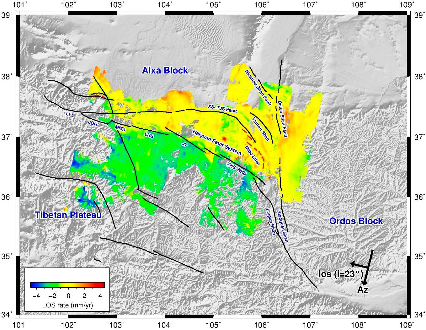
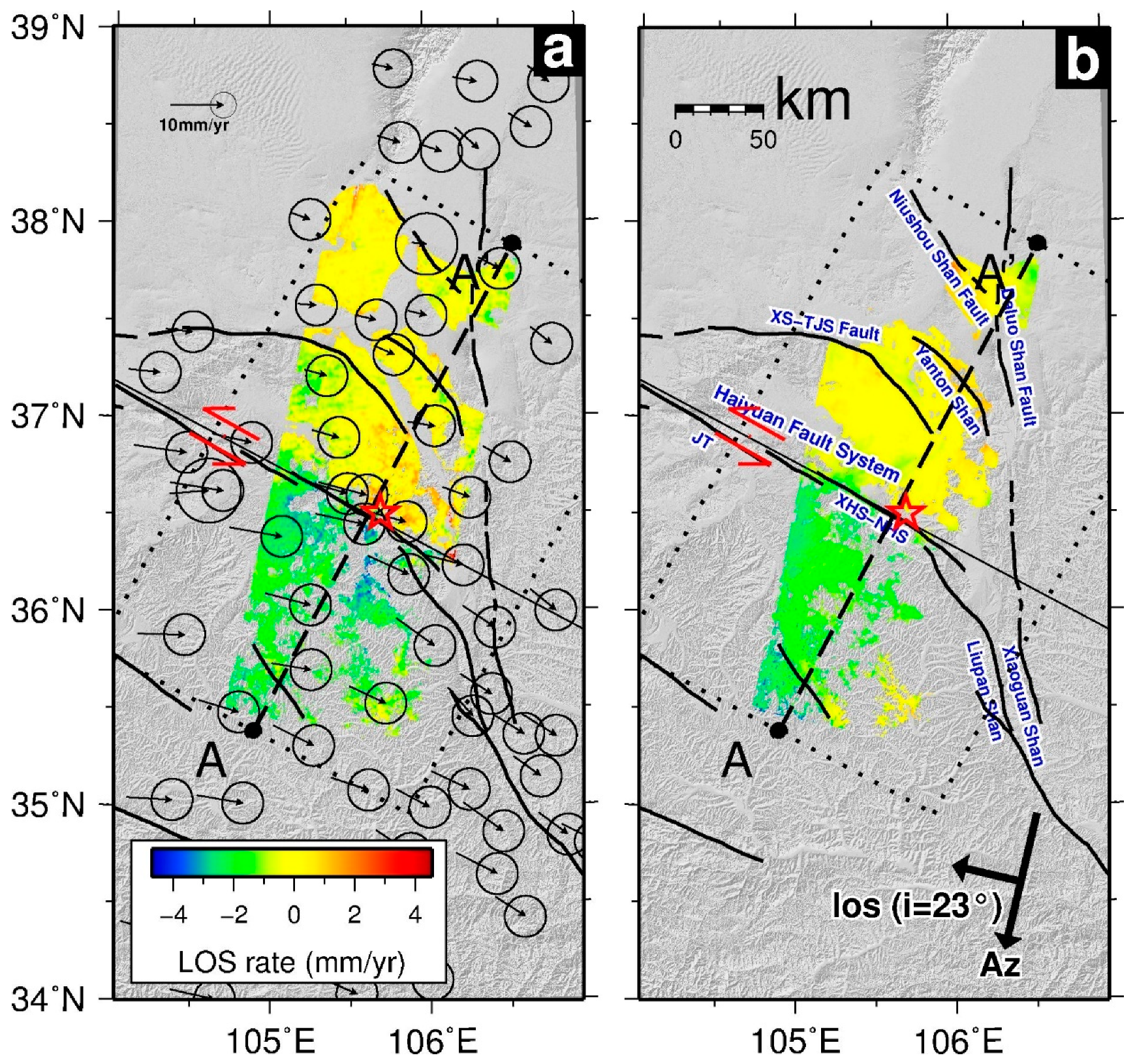
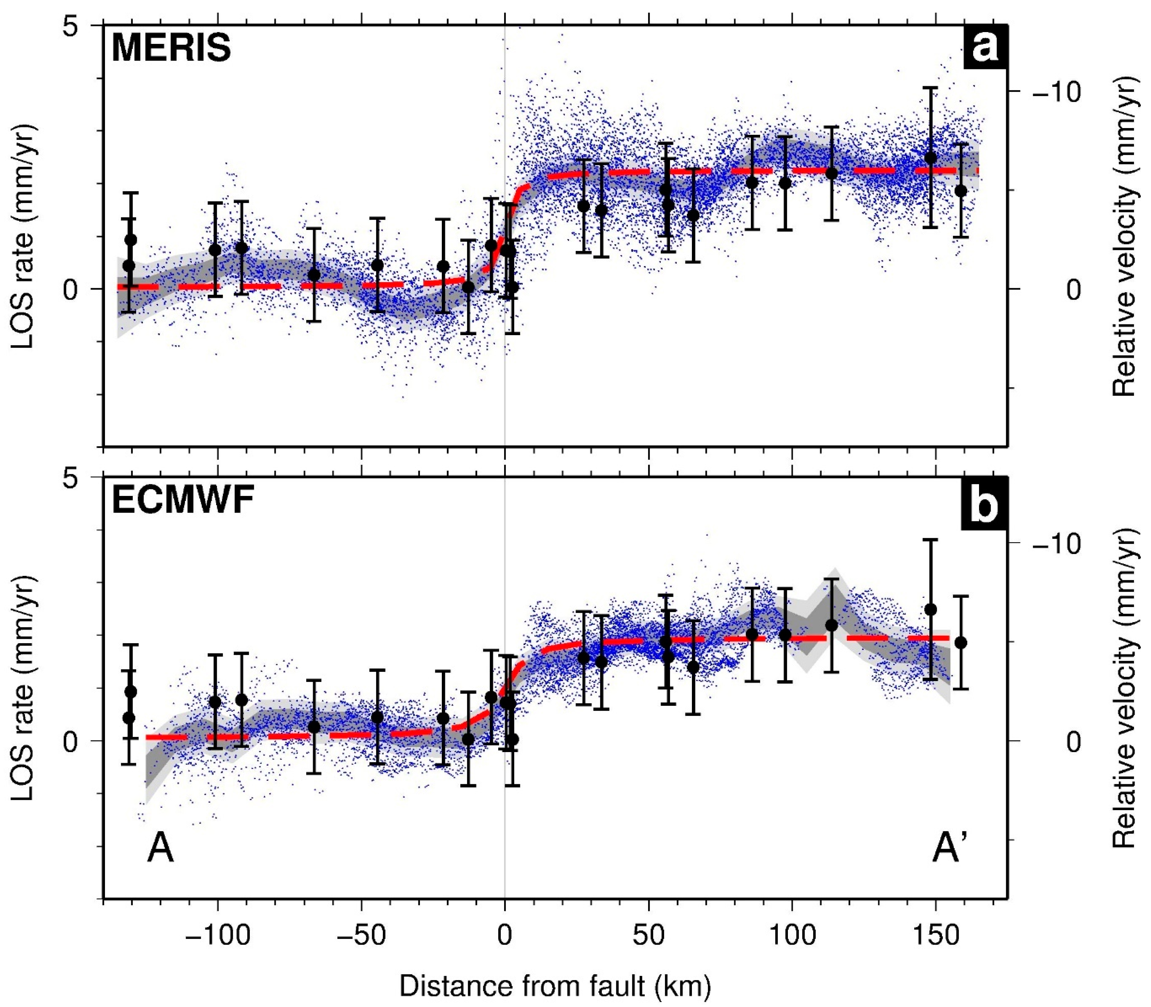
4. Construction of the InSAR Rate Map

For each Envisat ASAR track we collected, we constructed an interferometric stack composed of several chains of small-baseline interferograms, then applied the stacking InSAR method with atmospheric and orbital correction described in Section 3.1, to construct a deformation ratemap. Track 18 was chosen as an example to show the accuracy and reliability assessment of our results. Based on the baseline distribution of the track 18 (Figure S1), we constructed 3 chains of small-baseline interferograms (including 5 interferograms), which are completely composed of largely cloud-free SAR acquisitions, in order to make sure that the atmospheric contribution in each interferogram can be removed correctly using MERIS data (300 m spatial resolution). Following the steps mentioned above, A MERIS-corrected ratemap is achieved (Figure 3a). A rapid increase in the line-of-sight rate of deformation (∼2 mm/year) in a relatively narrow region across the Haiyuan fault can be seen, qualitatively consistent with left-lateral slip. There is no clear gradient in displacement rate related to tectonic signal on other faults north of the Haiyuan fault. GPS velocities were also projected into the local InSAR LOS direction and agree with the InSAR observations within the errors of the two measurements (see Figure 4). The RMS between the InSAR result and GPS is 0.6 mm/year.

In order to further validate our results using the MERIS corrections for atmospheric path delays, we also examined the ECMWF numerical weather model results for the region. Applying the method of Walters et al. [14], we produced atmospheric delay maps from ECMWF model results for each SAR acquisition. We compared the wet path delay maps derived from MERIS and ECMWF for the times of all the SAR acquisitions. A strong correlation was found between the ECMWF and MERIS-derived wet delay maps for 10 cloud-free acquisitions (Figure S3) in this area, with a mean correlation coefficient of 0.79 (ranging from 0.52 to 0.92), and a mean RMS misfit of 1 cm. There is also a good correlation for partially and largely cloudy acquisitions, although with a more limited number of data points. This suggests that the ECMWF atmospheric delay is potentially an alternative to MERIS data for correcting interferograms for atmospheric effects in this region.

In order to test the reliability and usefulness of the ECMWF data, we selected 13 interferograms (covering a total cumulative time of 40 years, see Figure S1) not included in the MERIS chains, and stacked 7 chains of these interferograms using the ECMWF correction for atmospheric effects. The ECMWF-corrected result (Figure 3b) agrees well with the MERIS-corrected result.

Following the steps mentioned above, we processed 12 Envisat ASAR acquisitions from descending track 247, which partially overlaps with track 18. A total of 36 interferograms with baselines of less than 200 m were produced, but only 3 of these showed good enough coherence. Subsequent analysis was based on these 3 interferograms alone. No cloud-free MERIS data is available for the acquisitions on track 247. But because the atmospheric correction based on the ECMWF model works well for track 18, we applied it to the interferograms for track 247 as well. After removing the atmospheric delays in this way and also removing an orbital ramp, we stacked the interferograms to create a ratemap for this track (Figure 5a). Even though only 3 interferograms from track 247 were used, the resulting ratemap agrees very well with the results from track 18. We compared the rates of range change in the overlapping area between the two swaths (Figure 5b). The two independent results show a very similar pattern with an offset of 2 mm/year in the LOS direction. This suggests that it is the quality of the interferograms that matters, and it is possible to measure slow ground motion with a very limited number of interferograms in this area, provided that appropriate corrections can be made for atmospheric effects.

From the experiments above, we can see that the stacking method with atmospheric and orbital correction proposed in this study works well in the Haiyuan fault zone, which is shown by: (1) the consistency between the MERIS-corrected and ECMWF-corrected ratemap (Figure 3), (2) consistency between the results from two adjacent tracks (Figure 5), and (3) consistency between InSAR and GPS (Figure 4). Therefore, applying this method to the other 5 tracks, we retrieved an InSAR ratemap for the most part of the Northeastern Tibetan area (Figure 6).

5. Inversion Results from InSAR and GPS

In order to obtain the detailed variations of deformation velocity near the faults, which may be observed by the high-resolution InSAR data, the whole Northeastern Tibetan area was meshed into an irregular grid by using the free software DistMesh [49]. Some points on the Haiyuan and other faults in this region were extracted to be used as the fixed points in discretization. A nominal mesh spacing of 0.05° was used to define the mesh density near the fault. An unstructured mesh was generated with different mesh density varying with the distance from the fault, i.e., dense points near the fault and sparse points far from the fault (Figure S4). Applying the algorithm presented in the Section 3, the horizontal velocities and strain rates on each node of the mesh were inverted from InSAR and GPS data. To avoid the effect from the nonelastic strain accumulation caused by the fault creep, we set the creeping section (103.68° E, 37.11° N to 104.15° E, 37.00° N) of the Haiyuan fault (Laohu Shan segment) identified by Jolivet et al. [17] as the barrier section.

Figure 7 shows the resulting horizontal strain rate field and principal compressive /tensile stress direction map, and Figure S5 shows the resulting velocity field. In general, the Northeastern Tibetan Plateau rotates clockwise (Figure S5), and the velocity decreases from south to north. Compared with the other faults in the north, the Haiyuan fault is the most active one, which demonstrates it is still an important boundary fault for the N-NW expansion of the Tibetan Plateau. This is in agreement with the geological research [24]. The difference between our study and geological studies [25,26] is that the present-day slip rate on the Haiyuan fault system varies little from west to east. A change (2–3 mm/year) in line-of-sight (LOS) deformation rate across the fault is observed from Jiangqianghe segment to its eastern end, where the northward expansion of the Plateau is transferring into shortening along the Liupan Shan fault due to the obstruction of the Alxa block in the north and Ordos block in the east.

From the horizontal strain rate field (Figure 7a), strain accumulation is strongly localized on the left-lateral strike-slip Haiyuan fault zone. This is similar to the discovery of previous studies on the Karakoram fault [10] and the Anatolia fault [1]. Wright et al. [50] suggests that strain accumulation in inter-seismic stage is a major feature of large strike-slip faults. High strain rate regions also are observed to follow the other faults in the north, although the magnitude is smaller than that of strain rate on the Haiyuan fault. Benefit from high spatial resolution InSAR ratemap, some detail strain rate variation near the fault can be detected, which can not be observed by GPS only as shown in Li et al. [51]. In Figure 8, an interesting phenomenon caused by the fault creep is revealed clearly by our fine strain rate field. The creeping segment reveal by our InSAR and Jolivet et al. [17] located at a low strain accumulation zone, instead the areas next to its two ends are holding a high strain rate.

From the direction of principal stress (Figure 7b), the Haiyuan fault system is dominated by a strike-slip motion with a relatively small thrust component (please note that the pink E-W strike-slip components is covered by the black thrusting components), which is consistent with the focal mechanism of the moderate earthquakes happened on it in recent decades (Figure S6). An abnormal tension zone can be see along the Daluo Shan fault, which is contrary to the previous knowledge of squeezing structure. Recent geological study [52] confirm that there exists a normal faulting component in the junction between the Niushou Shan fault and Daluo Shan fault. The regional seismicity map also shows that a Mw 5.3 earthquake with normal faulting occurred nearby on 10 August 1987 (Figure S6). We also note that the southern part of the Liupan Shan fault shows a dominating extension that is out of our expectation. That is because local GPS observation dominates the inversion result in absence of high-coherenced InSAR data in this region, where one of GPS velocity in the west of the fault is small than the ones in the east (Figure S7), thus caused a tensional stress zone.

6. Discussion

6.1. The Present-Day Kinematics for the Rupture of the 1920 Earthquake

To study the present-day fault movement of the 1920 rupture, we constructed fault-perpendicular profiles across the atmospheric-corrected ratemaps from the track 18 covered the 1920 rupture. We projected all LOS velocities onto this profile, then a conventional screw dislocation arctan model [53] was used to invert for the best-fitting slip rate and locking depth. The minimum misfit corresponds to a best-fitting model with slip rate of 5.9 mm/year and locking depth of 3 km shown by the dashed red line in Figure 4a for the MERIS-corrected ratemap. The inversion for the ECMWF-corrected ratemap gives a similar result (Figure 4b: a slip rate of 5 mm/year with a locking depth of 6 km). Our InSAR results are consistent with the GPS velocity of 4.2 ± 1.5 mm/year given by Zheng et al. [29], and Holocene slip rate of 4.5 ± 2 mm/year given by Li et al. [30].

A shallow locking depth is often linked to creep at shallow depths. This kind of creep might be disconnected from the steadily slipping section below the seismogenic depth [16]. Such creeping behavior has been observed on the western end of the 1920 rupture, i.e., the Laohu Shan segment [16,17,18]. Our inversions show a shallow locking depth (3–6 km) for the main rupture zone of the 1920 earthquake. Our InSAR profiles (Figure 4 and Figure 5) also show that the LOS velocities vary rapidly in a relative narrow zone across the fault, but not as sharp as in the Laohu Shan segment (~5 km) showed in Jolivet et al. [17]. We therefore infer that the middle-lower part of the seismogenic layer on the 1920 rupture is not yet fully locked since the 1920 large earthquake, which may explain why no moderate earthquakes have ever occurred here since 1920. The question remains whether it is caused by the creep or by the post-seismic afterslip, which may be answered by more observations in future decades.

6.2. Expansion Frontier of the Northeastern Tibet Plateau

Previous studies suggested that the northeastern Tibet is expanding laterally since the late Cenozoic (20–10 Ma), which is partly accommodated by the left-lateral strike-slip along the East Kunlun and Haiyuan faults and crustal shortening of the Tibet–Ordos transition zone [54]. It is still controversial about the route and scale of lateral motion caused by the outward growth of the Northeastern Tibetan Plateau. Some studies suggested that the Plateau is extruding laterally along the EW trending Qinling tectonic zone [55,56], but some results argued that the ENE lateral expansion of the plateau has being penetrating into the southern margin of Ordos Block or even its interior due to spatial differences in the internal lithosphere structure of the Ordos [57,58,59]. From the distribution of principal stress (Figure 9) we achieved here, the expanding front of the northeastern plateau has crossed the Liupan Shan fault zone, even arrived at the northeast area of the Xiaoguan Shan. This is also revealed by deep seismic reflection profile. The deep crustal “architecture” suggests that the Xiaoguan Shan to the east of the Liupan Shan fault zone has been affected by the northeastward growth of the plateau [60].

7. Conclusions

We used InSAR, combined with two different estimates of atmospheric path delays, to estimate the interseismic strain accumulation across the Northeastern Tibetan Plateau. The results show that the MERIS-based and ECMWF-based corrections both work well in removing the atmospheric delays and retrieving the interseismic deformation, even when stacking with a smaller number of interferograms. The combination of InSAR and GPS observations has given refined estimates of the deformation velocity and strain rate field with a high spatial resolution in this region. It revealed the strain variation near the fault in great detail. Such a fine strain field enabled us to gain new insights about the present-day kinematics of the 1920 rupture and the lateral expansion of the northeastern Tibet Plateau. With more and more new satellites being operated, the combination of multi-satellites data with a timespan of a few decades will allow us to investigate time-dependent slip behavior of the fault, which enable us to discriminate different deformation mechanism.

References

1. Walters, R.J. Geodetic Observation and Modelling of Continental Deformation in Iran and Turkey. Ph.D. Thesis, University of Oxford, Oxford, UK, 2012. [Google Scholar]
2. Funning, G.J.; Parsons, B.; Wright, T.J.; Jackson, J.A.; Fielding, E.J. Surface displacements and source parameters of the 2003 Bam (Iran) earthquake from Envisat advanced synthetic aperture radar imagery. J. Geophys. Res. 2005, 110, B09. [Google Scholar] [CrossRef]
3. Li, Z.; Elliott, J.R.; Feng, W.; Jackson, J.A.; Parsons, B.; Walters, R.J. The 2010 Mw 6.8 Yushu (Qinghai, China) earthquake: Constraints provided by InSAR and body wave seismology. J. Geophys. Res. 2011, 116, B10302. [Google Scholar] [CrossRef]
4. Elliott, J.; Jolivet, R.; González, P.; Avouac, J.-P.; Hollingsworth, J.; Searle, M.; Stevens, V. Himalayan megathrust geometry and relation to topography revealed by the Gorkha earthquake. Nat. Geosci. 2016, 9, 174–180. [Google Scholar] [CrossRef] [Green Version]
5. Atzori, S.; Manunta, M.; Fornaro, G.; Ganas, A.; Salvi, S. Postseismic displacement of the 1999 Athens earthquake retrieved by the Differential Interferometry by Synthetic Aperture Radar time series. J. Geophys. Res. 2008, 113, B09309. [Google Scholar] [CrossRef]
6. Gonzalez-Ortega, A.; Fialko, Y.; Sandwell, D.; Alejandro Nava-Pichardo, F.; Fletcher, J.; Gonzalez-Garcia, J.; Lipovsky, B.; Floyd, M.; Funning, G. ElMayor-Cucapah (Mw7.2) earthquake:Early near-field postseismic deforma-tion from InSAR and GPS observations. J. Geophys. Res. Solid Earth 2014, 119. [Google Scholar] [CrossRef]
7. Kyriakopoulos, C.; Chini, M.; Bignami, C.; Stramondo, S.; Ganas, A.; Kolligri, M.; Moshou, A. Monthly migration of a tectonic seismic swarm detected by DInSAR: Southwest Peloponnese, Greece. Geophys. J. Int. 2013, 194, 1302–1309. [Google Scholar] [CrossRef]
8. Wicks, C.; Thelen, W.; Weaver, C.; Gomberg, J.; Rohay, A.; Bodin, P. InSAR observations of aseismic slip associated with an earthquake swarm in the Columbia River flood basalts. J. Geophys. Res. 2011, 116, B12304. [Google Scholar] [CrossRef]
9. Elliott, J.R.; Biggs, J.; Parsons, B.; Wright, T.J. InSAR slip rate determination on the Altyn Tagh Fault, northern Tibet, in the presence of topographically correlated atmospheric delays. Geophys. Res. Lett. 2008, 35, L12309. [Google Scholar] [CrossRef]
10. Wang, H.; Wright, T. Satellite geodetic imaging reveals internal deformation of western Tibet. Geophys. Res. Lett. 2012, 39, L07303. [Google Scholar] [CrossRef]
11. Tong, X.; Sandwell, D.T.; Smith-Konter, B. High-resolution interseismic velocity data along the San Andreas fault from GPS and InSAR. J. Geophys. Res. 2013, 118, 369–389. [Google Scholar] [CrossRef]
12. Jin, L.; Funning, G.J. Testing the inference of creep on the northern Rodgers Creek fault, California, using ascending and descending persistent scatterer InSAR data. J. Geophys. Res. 2017, 122, 2373–2389. [Google Scholar] [CrossRef]
13. Xu, W.; Wu, S.; Materna, K.; Nadeau, R.; Floyd, M.; Funning, G.; Chaussard, E.; Johnson, C.W.; Murray, J.R.; et al. Interseismic ground deformation and fault slip rates in the greater San Francisco bay area from two decades of space geodetic data. J. Geophys. Res. 2018, 123, 8095–8109. [Google Scholar] [CrossRef]
14. Walters, R.J.; Holley, R.J.; Parsons, B.; Wright, T.J. Interseismic strain accumulation across the North Anatolian Fault from Envisat InSAR measurements. J. Geophys. Res. 2011, 38. [Google Scholar] [CrossRef] [Green Version]
15. Kaneko, Y.; Fialko, Y.; Sandwell, D.T.; Tong, X.; Furuya, M. Interseismic deformation and creep along the central section of the North Anatolian Fault (Turkey): InSAR observations and implications for rate-and-state friction properties. J. Geophys. Res. 2013, 118, 316–331. [Google Scholar] [CrossRef] [Green Version]
16. Cavalié, O.; Lasserre, C.; Doin, M.-P.; Peltzer, G.; Sun, J.; Xu, X.; Shen, Z.-K. Measurement of interseismic strain across the Haiyuan fault (Gansu, China), by InSAR. Earth Planet. Sci. Lett. 2008, 275, 246–257. [Google Scholar] [CrossRef]
17. Jolivet, R.; Lasserre, C.; Doin, M.-P.; Guillaso, S.; Peltzer, G.; Dailu, R.; Sun, J.; Shen, Z.-K.; Xu, X. Shallow creep on the Haiyuan Fault (Gansu, China) revealed by SAR Interferometry. J. Geophys. Res. 2012, 117, B06401. [Google Scholar] [CrossRef]
18. Jolivet, R.; Lasserre, C.; Doin, M.-P.; Peltzer, G.; Avouac, J.-P.; Sun, J.; Dailu, R. Spatio-temporal evolution of aseismic slip along the Haiyuan fault, China: Implications for fault frictional properties. Earth Planet. Sci. Lett. 2013, 377, 23–33. [Google Scholar] [CrossRef]
19. Daout, S.; Jolivet, R.; Lasserre, C.; Doin, M.P.; Barbot, S.; Tapponnier, P.; Peltzer, G.; Socquet, A.; Sun, J. Along-strike variations of the partitioning of convergence across the Haiyuan fault system detected by InSAR. Geophys. J. Int. 2016, 205, 536–547. [Google Scholar] [CrossRef]
20. Zhang, P.; Molnar, P.; Burchfiel, B.C.; Royden, L.; Wang, Y.; Deng, Q.; Song, F.; Zhang, W.; Jiao, D. Bounds on the Holocene slip rate of the Haiyuan fault, north-central China. Quat. Res. 1988, 30, 151–164. [Google Scholar]
21. Gaudemer, Y.; Tapponnier, P.; Meyer, B.; Peltzer, G.; Guo, S.; Chen, Z. Partitioning of crustal slip between linked, active faults in the eastern Qilian Shan, and evidence for a major seismic gap, the ‘Tianzhu gap’, on the western Haiyuan fault, Lanzhou (China). Geophys. J. Int. 1995, 120, 599–645. [Google Scholar] [CrossRef]
22. Gan, W.; Zhang, P.; Shen, Z.-K.; Niu, Z.; Wang, M.; Wan, Y.; Zhou, D.; Cheng, J. Present-day crustal motion within the Tibetan Plateau inferred from GPS measurements. J. Geophys. Res. 2007, 112, B08416. [Google Scholar] [CrossRef]
23. Burchfiel, B.; Zhang, P.; Wang, Y.; Zhang, W.; Song, F.; Deng, Q.; Molnar, P.; Royden, L. Geology of the Haiyuan fault zone, Ningxia-Hui Autonomous Region, China, and its relation to the evolution of the northeastern margin of the Tibetan Plateau. Tectonics 1991, 10, 1091–1110. [Google Scholar] [CrossRef]
24. Zhang, P.; Burchfiel, B.; Molnar, P.; Zhang, W.; Jiao, D.; Deng, Q.; Wang, Y.; Royden, L.; Song, F. Late Cenozoic tectonic evolution of the Ningxia-Hui autonomous region, China. Geol. Soc. Am. Bull. 1990, 102, 1484–1498. [Google Scholar]
25. Lasserre, C.; Morel, P.-H.; Gaudemer, Y.; Tapponnier, P.; Ryerson, F.; King, G.; Métivier, F.; Kasser, M.; Kashgarian, M.; Liu, B.; et al. Postglacial left slip rate and past occurrence of M ≥ 8 earthquakes on the Western Haiyuan Fault, Gansu, China. J. Geophys. Res. Solid Earth 1999, 104, 17633–17651. [Google Scholar] [CrossRef]
26. Lasserre, C.; Gaudemer, Y.; Tapponnier, P.; Mériaux, A.-S.; Van der Woerd, J.; Daoyang, Y.; Ryerson, F.J.; Finkel, R.C.; Caffee, M.W. Fast late Pleistocene slip rate on the Leng Long Ling segment of the Haiyuan fault, Qinghai, China. J. Geophys. Res. 2002, 107, 2276. [Google Scholar] [CrossRef]
27. He, W.; Liu, B.; Lu, T.; Yuan, D.; Liu, J.; Liu, X. Study on the segmentation of Laohushan fault zone. Northwest. Seismol. J. 1994, 16, 66–72. [Google Scholar]
28. He, W.; Liu, B.; Yuan, D.; Yang, M. Research on slip rates of the Lenglongling active fault zone. Northwest. Seismol. J. 2000, 22, 90–97. [Google Scholar]
29. Zheng, W.J.; Zhang, P.Z.; He, W.G.; Yuan, D.Y.; Shao, Y.X.; Zheng, D.W.; Ge, W.P.; Min, W. Transformation of displacement between strike-slip and crustal shortening in the northern margin of the Tibetan Plateau: Evidence from decadal GPS measurements and late Quaternary slip rates on faults. Tectonophysics 2013, 584, 267–280. [Google Scholar] [CrossRef]
30. Li, C.; Zhang, P.; Yin, J.; Min, W. Late Quaternary left-lateral slip rate of the Haiyuan fault, northeastern margin of the Tibetan Plateau. Tectonics 2009, 28, TC5010. [Google Scholar] [CrossRef]
31. Farr, T.; Rosen, P.A.; Caro, E.; Crippen, R.; Duren, R.; Hensley, S.; Kobrick, M.; Paller, M.; Rodriguez, E.; Roth, L.; et al. Shuttle Radar Topography Mission. Rev. Geophys. 2007, 45, RG2004. [Google Scholar] [CrossRef]
32. Goldstein, R.M.; Zebker, H.A.; Werner, C.L. Satellite radar interferometry—Two-dimensional phase unwrapping. Radio Sci. 1988, 23, 713–720. [Google Scholar] [CrossRef]
33. Hanssen, R.F. Radar Interferometry: Data Interpretation and Analysis; Kluwer Academic: New York, NY, USA, 2001; pp. 130–148. [Google Scholar]
34. Zebker, H.A.; Rosen, P.A.; Hensley, S. Atmospheric effects in interferometric synthetic aperature radar surface deformation and topographic maps. J. Geophys. Res. 1997, 102, 7547–7564. [Google Scholar] [CrossRef]
35. Ferretti, A.; Prati, C.; Rocca, F. Permanent scatterers in SAR interferometry. IEEE Trans. Geosci. Remote Sens. 2001, 39, 8–20. [Google Scholar] [CrossRef] [Green Version]
36. Doin, M.-P.; Lasserre, C.; Peltzer, G.; Cavalié, O.; Doubre, C. Corrections of stratified tropospheric delays in SAR interferometry: Validation with global atmospheric models. J. Appl. Geophys. 2009, 69, 35–50. [Google Scholar] [CrossRef]
37. Li, Z.; Muller, J.P.; Cross, P.; Albert, P.; Fischer, J.; Bennartz, R. Assessment of the potential of MERIS near infrared water vapour products to correct ASAR interferometric measurements. Int. J. Remote Sens. 2006, 27, 349–365. [Google Scholar] [CrossRef]
38. Frank, F.C. Deduction of Earth strains from survey data. Bull. Seismol. Soc. Am. 1966, 56, 35–42. [Google Scholar]
39. Brunner, F.K.; Coleman, R.; Hirsch, B. A comparison of computation methods for crustal strains from geodetic measurements. Tectonophysics 1981, 71, 281–298. [Google Scholar] [CrossRef]
40. Haines, A.J.; Holt, W.E. A procedure for obtaining the complete horizontal motions within zones of distributed deformation from the inversion of strain rate data. J. Geophys. Res. 1993, 98, 12057–12082. [Google Scholar] [CrossRef]
41. Holt, W.E.; Chamot-Rooke, N.; LePichon, X.; Haines, A.J.; Shen-Tu, B.; Ren, J. Velocity field in Asia inferred from quaternary fault slip rates and global positioning system observations. J. Geophys. Res. 2000, 105, 19185–19209. [Google Scholar] [CrossRef]
42. Kreemer, C.; Holt, W.E.; Haines, A.J. An integrated global model of present-day plate motions and plate boundary deformation. Geophys. J. Int. 2003, 154, 8–34. [Google Scholar] [CrossRef] [Green Version]
43. Wessel, P.; Becker, J.M. Interpolation using a generalized Green’s function for a spherical surface spline in tension. Geophys. J. Int. 2008, 174, 21–28. [Google Scholar] [CrossRef]
44. Noda, A.; Matsu’ura, M. Physics-based GPS data inversion to estimate three-dimensional elastic and inelastic strain fields. Geophys. J. Int. 2010, 182, 513–530. [Google Scholar] [CrossRef] [Green Version]
45. Kreemer, C.; Blewitt, G.; Klein, E.C. A geodetic plate motion and global strain rate model. Geochem. Geophys. Geosyst. 2014, 15, 3849–3889. [Google Scholar] [CrossRef]
46. Shen, Z.-K.; Jackson, D.D.; Ge, B.X. Crustal deformation across and beyond the Los Angeles basin from geodetic measurements. J. Geophys. Res. 1996, 101, 27957–27980. [Google Scholar] [CrossRef] [Green Version]
47. Shen, Z.-K.; Jackson, D.D.; Kagan, Y.Y. Implications of geodetic strain rate for future earthquakes, with a five-year forecast of M 5 earthquakes in southern California. Seismol. Res. Lett. 2007, 78, 117–120. [Google Scholar] [CrossRef]
48. Shen, Z.K.; Wang, M.; Zeng, Y.; Wang, F. Optimal interpolation of spatially discretized geodetic data. Bull. Seismol. Soc. Am. 2015, 105, 2117–2127. [Google Scholar] [CrossRef]
49. Persson, P.O.; Strang, G. A simple mesh generator in MATLAB. SIAM Rev. 2004, 46, 329–345. [Google Scholar] [CrossRef]
50. Wright, T.J.; Elliott, J.R.; Wang, H.; Ryder, I. Earthquake cycle deformation and the Moho: Implications for the rheology of continental lithosphere. Tectonophysics 2013, 609, 504–523. [Google Scholar] [CrossRef] [Green Version]
51. Li, Y.; Shan, X.; Qu, C.; Zhang, Y.; Song, X.; Jiang, Y.; Zhang, G.; Nocquet, J.M.; Gong, W.; Gan, W.; et al. Elastic block and strain modeling of GPS data around the Haiyuan-liupanshan fault, northeastern Tibetan Plateau. J. Asian Earth Sci. 2017, 150, 87–97. [Google Scholar] [CrossRef]
52. Lei, Q.Y. The Extension of the Arc Tectonic Belt in the Northeastern Margin of the Tibet Plateau and the Evolution of the Yinchuan Basin in the Western Margin of the North China. Ph.D. Thesis, Institute of Geology, China Earthquake Administration, Beijing, China, 2016. [Google Scholar]
53. Savage, J.C.; Burford, R.O. Geodetic Determination of Relative Plate Motion in Central California. J. Geophys. Res. 1973, 78, 832–845. [Google Scholar] [CrossRef]
54. Yuan, D.Y.; Ge, W.P.; Chen, Z.W.; Li, C.Y.; Wang, Z.C.; Zhang, H.P.; Zhang, P.Z.; Zheng, D.W.; Zheng, W.J.; Craddock, W.H.; et al. The growth of northeastern Tibet and its relevance to large scale continental geodynamics: A review of recent studies. Tectonics 2013, 32, 1358–1370. [Google Scholar] [CrossRef]
55. Tapponnier, P.; Xu, Z.Q.; Roger, F.; Meyer, B.; Arnaud, N.; Wittlinger, G.; Jingsui, Y. Oblique stepwise rise and growth of the Tibet Plateau. Science 2001, 294, 1671–1677. [Google Scholar] [CrossRef]
56. Zuza, A.V.; Yin, A. Continental deformation accommodated by non-rigid passive bookshelf faulting: An example from the Cenozoic tectonic development of northern Tibet. Tectonophysics 2016, 677–678, 227–240. [Google Scholar] [CrossRef]
57. Wang, C.Y.; Sandvol, E.; Zhu, L.; Lou, H.; Yao, Z.; Luo, X. Lateral variation of crustal structure in the Ordos block and surrounding regions, North China, and its tectonic implications. Earth Planet. Sci. Lett. 2014, 387, 198–211. [Google Scholar] [CrossRef]
58. Tang, Y.; Zhou, S.; Chen, Y.J.; Sandvol, E.; Liang, X.; Feng, Y.; Jin, G.; Jiang, M.; Liu, M. Crustal structures across the western Weihe Graben, North China: Implications for extrusion tectonics at the northeast margin of Tibetan Plateau. J. Geophys. Res. 2015, 120, 5070–5081. [Google Scholar] [CrossRef] [Green Version]
59. Li, Y.H. Study on the Lateral Motion of Northeastern Tibetan Plateau. Ph.D. Thesis, Institute of Geology, China Earthquake Administration, Beijing, China, 2017. [Google Scholar]
60. Guo, X.Y.; Gao, R.; Wang, H.; Li, W.; Keller, G.R.; Xu, X.; Li, H.; Encarnacion, J. Crustal architecture beneath the Tibet-Ordos transition zone, NE Tibet, and the implications for plateau expansion. Geophys. Res. Lett. 2015, 42, 10631–10639. [Google Scholar] [CrossRef]
Figure 1. Tectonic map of the northeastern margin of the Tibetan Plateau. The major Haiyuan fault system is composed of several segments: LLL Leng Long Ling, JQH Jing Qiang He, MMS Maomao Shan, LHS Laohu Shan, JT Jing Tai, XHS-NHS Xihua Shan-Nanhua Shan, XS-TJS Xiang Shan-Tianjing Shan. The thick black solid lines indicate active faults in Holocene. The red solid circle represents the epicenter of the 1920 earthquake; the red solid lines show its surface rupture. Black rectangles show the coverage of Envisat ASAR data, with track numbers indicated. GPS data with respect to the Eurasia-fixed Reference Frame is from Gan et al. [22].
Remotesensing 11 00435 g001
Figure 2. A flowchart for stacking interferometric synthetic aperture radar (InSAR) with atmospheric-corrected interferograms.
Remotesensing 11 00435 g002
Figure 3. (a) Mean line-of-sight (LOS) ratemap for track 18 produced from MERIS-corrected interferograms indicated by red line in Figure S1. A positive LOS displacement corresponds to movement away from the satellite. A-A’ marks the profile shown in Figure 4a. GPS data with respect to the Eurasia-fixed Reference Frame is from Gan et al. [22]. (b) Mean LOS ratemap for track 18 produced from ECMWF-corrected interferograms indicated by green line in Figure S1. The perpendicular pair of arrows shows the direction in which the satellite moves (Az), the satellite line-of-sight direction (los), and the incidence angle (i) at the centre of the scene. JT: Jing Tai fault, XHS-NHS: Xihua Shan-Nanhua Shan fault, XS-TJS: Xiang Shan-Tianjing Shan.
Remotesensing 11 00435 g003
Figure 4. (a) Average rate profile produced by projecting all points of the MERIS-corrected rate-map onto the line A-A’ indicated in Figure 2. The thick grey bands show the 1- and 2-σ error bounds on LOS rate. Blue points are individual pixels from the rate-map. Black bars are the horizontal GPS velocities and error bounds shown in the footprint of track 18 in Figure 2, and converted into satellite LOS rates. Velocities predicted by our best-fit slip model are plotted as a red dashed line. (b) Same as for (a) but for ECMWF-corrected rate-map indicated in Figure 2.
Remotesensing 11 00435 g004
Figure 5. (a) Mean LOS ratemap for track 18 and 247, produced by stacking the MERIS-corrected and ECMWF-corrected interferograms respectively. The white line shows the profile centre for the profile presented in the right panel. The black dashed box shows the overlapping area between track 18 and 247. JT: Jing Tai fault, XHS-NHS: Xihua Shan-Nanhua Shan fault, XS-TJS: Xiang Shan-Tianjing Shan fault. (b) Rate profile for a 40 km-wide swath (black dashed box in the left panel) centered on the line B-B’. The blue points are individual pixels from the ratemap of track 18, red points from track 247, and the green line shows the mean velocity of the two datasets.
Remotesensing 11 00435 g005
Figure 6. InSAR Mean LOS ratemap for 6 tracks covered the northeastern margin of the Tibetan Plateau, produced by stacking the atmospheric-corrected interferograms. LLL: Leng Long Ling, JQH: Jing Qiang He, MMS: Maomao Shan, LHS: Laohu Shan, JT: Jing Tai, XHS-NHS: Xihua Shan-Nanhua Shan, XS-TJS: Xiang Shan-Tianjing Shan.
Remotesensing 11 00435 g006
Figure 7. Results inverted jointly by InSAR and GPS for the northeastern margin of the Tibetan Plateau. (a) The horizontal strain rate field: the magnitude of second invariant of the strain rate tensor. The black dashed boxes show the areas for the Figure 8 and Figure 9. LLL: Leng Long Ling, JQH: Jing Qiang He, MMS: Maomao Shan, LHS: Laohu Shan, JT: Jing Tai, XHS-NHS: Xihua Shan-Nanhua Shan, XS-TJS: Xiang Shan-Tianjing Shan. (b) The principal compressive/tensile stress direction map. The short black lines are for compressive stress and the pink lines are for the tensile stress.
Remotesensing 11 00435 g007
Figure 8. The horizontal strain rate (the second invariant of the strain rate tensor) distribution in Laohu Shan fault zone and its surrounding area. The grey lines indicate the Haiyuan fault system (JQH: Jing Qiang He, MMS: Maomao Shan, LHS: Laohu Shan, JT: Jing Tai). The red line indicates the creeping segment identified by Jolivet et al. [17], and GCMT focal mechanisms are given for four moderate earthquakes occurred in this region in the past 30 years.
Remotesensing 11 00435 g008
Figure 9. The horizontal strain rate (the second invariant of the strain rate tensor) distribution for the Tibet–Ordos transition zone. The grey lines indicate the fault line (XHS-NHS: Xihua Shan-Nanhua Shan). The short black/pink lines are the principal compressive/tensile stress directions.
Remotesensing 11 00435 g009