Article

Ship Classification Based on Multifeature Ensemble with Convolutional Neural Network

1
College of Information Science and Technology, Beijing University of Chemical Technology, Beijing 100029, China
2
School of Information and Electronics, Beijing Institute Technology, Beijing 100081, China
3
Institute of Remote Sensing and Digital Earth, Chinese Academy of Science, Beijing 100094, China
*
Author to whom correspondence should be addressed.
Remote Sens. 2019, 11(4), 419; https://doi.org/10.3390/rs11040419
Submission received: 7 January 2019 / Revised: 10 February 2019 / Accepted: 12 February 2019 / Published: 18 February 2019
(This article belongs to the Special Issue AI-based Remote Sensing Oceanography)

Abstract

:
As an important part of maritime traffic, ships play an important role in military and civilian applications. However, ships’ appearances are susceptible to some factors such as lighting, occlusion, and sea state, making ship classification more challenging. This is of great importance when exploring global and detailed information for ship classification in optical remote sensing images. In this paper, a novel method to obtain discriminative feature representation of a ship image is proposed. The proposed classification framework consists of a multifeature ensemble based on convolutional neural network (ME-CNN). Specifically, two-dimensional discrete fractional Fourier transform (2D-DFrFT) is employed to extract multi-order amplitude and phase information, which contains such important information as profiles, edges, and corners; completed local binary pattern (CLBP) is used to obtain local information about ship images; Gabor filter is used to gain the global information about ship images. Then, deep convolutional neural network (CNN) is applied to extract more abstract features based on the above information. CNN, extracting high-level features automatically, has performed well for object classification tasks. After high-feature learning, as the one of fusion strategies, decision-level fusion is investigated for the final classification result. The average accuracy of the proposed approach is 98.75% on the BCCT200-resize data, 92.50% on the original BCCT200 data, and 87.33% on the challenging VAIS data, which validates the effectiveness of the proposed method when compared to the existing state-of-art algorithms.

1. Introduction

Ship classification in optical remote sensing imagery is important for enhancing maritime safety and security [1,2]. However, the appearance of ships is easily affected by natural factors such as cloud, sunlight, etc., and wide variations within class in some types of ships and viewing geometry, which make the improvement of the efficiency of ship classification more challenging and complicated [3,4].
Over the last decade, different kinds of feature extraction algorithms have been proposed to solve the problem of ship classification using remote sensing images. For example, principal components analysis (PCA) [5], as the one of most popular tools in feature extraction and dimensionality reduction, was employed to ship classification. Then, linear discriminant analysis (LDA) was also used in vessel recognition [6], which can make better use of class information to maximize inter-class dispersion and minimize intra-class dispersion compared with PCA. In [7], hierarchical multi-scale local binary pattern (HMLBP) was applied to extract local features. In [8], histogram of oriented gradients (HOG) was adopted to extract features because it is a better image descriptor, able to capture the local object appearance and shape in the image. In [9], the bag of visual words (BOVW) was employed in vessel classification, which is inspired by the bag of words representation used in text classification tasks. In [10], Rainey et al. proposed several object recognition algorithms to classify the category of vessel, which obtained good results. In [11], the local binary patterns (LBP) operator was developed for vessel classification. In [12], the completed local binary patterns (CLBP) was proposed to overcome the shortcoming of LBP. Furthermore, the multiple features learning (MFL) framework [13], including Gabor-based multi-scale completed local binary pattern (MS-CLBP), patch-based MS-CLBP and Fisher vector (FV) [14], and BOVW-based spatial pyramid matching (SPM), were all presented for ship classification. Gabor filtering has been employed in some object recognition tasks, such as facial expression recognition [15] and image classification [16].
Compared with the Gabor filter, fractional Fourier transform (FrFT) has lower computational complexity and time-frequency focusing characteristics. As a generalization of conventional Fourier transform, the FrFT is a powerful and effective tool for time-frequency analysis, including time-frequency characteristics of the signal [17]. FrFT executes a rotation of signal to any angle, while the conventional Fourier transform is just a π / 2 rotation in the frequency plane. Therefore, it is regarded as an appropriate representation of the chirp signal and has been widely used in the field of signal processing [18,19]. In 2001, two-dimensional discrete FrFT (2D-DFrFT) was presented to accomplish optical image encryption [20]. 2D-DFrFT can capture more characters of a face image in different angles, and the lower-frequency bands contain most facial discriminating features, while high bands contain the noise. Thus, it has been employed in face recognition [21], human emotional state recognition [22] and facial expression recognition [23], and obtained good results.
Recently, convolutional neural network (CNN) has shown great potential in the field of vision recognition tasks by learning high-level features from raw data via convolution operation automatically [24,25,26]. CNN is an application of deep learning algorithms in the field of image processing [27]. A powerful part of deep learning is that the output of one layer in the middle can be regarded as another expression of data. Compared with the above hand-crafted features, it has the following advantages: first, the process of feature extraction and classification is dependent, which means the results can be fed back for learning better features; second, the features extracted by CNN have a lower complexity image. CNN has been employed successfully in the field of computer vision, including image classification [28,29,30], which demonstrates excellent performance. Although CNN has performed promisingly, it also carries some limitations: firstly, the CNN learning feature is based on low-level features obtained in the first convolution layer, which may cause some important information to be lost, such as edge, contour, and so on. Secondly, it cannot learn global rotation-invariant features of ship images [31,32], which is of importance for classifying vessel category. Thirdly, because the bottom of CNN acquires information such as image edge, when the edge of the image is not clear, it cannot achieve good results.
Therefore, to overcome these shortcomings, a multifeature ensemble based on convolutional neural network (ME-CNN) framework, which combines multi-diversity in hand-crafted features with the advantage of high-level features in CNN, is presented to classify the category of ship types. The proposed method employs 2D-DFrFT in the preprocessing stage to produce amplitude and phase information of different orders. Signal-order features are not enough to classify the image type and 2D-DFrFT features of various orders extracted from the same image usually reflect different characteristic of the original image. Therefore, it is important to combine various multi-order features, which not only obtains more discriminative descriptions of multi-order features, but also eliminates redundant information about certain angles. Gabor filtering has an excellent ability to represent the spatial structures of different scales and orientations, which is employed when extracting global rotation-invariant features. Since CLBP can extract detailed local structure and texture information in images, it is used to obtain local texture information about the ship image. In this paper, multi-order features, including amplitude and phase information, and Gabor feature and CLBP images, are viewed as inputs of the CNN to obtain excellent performance. Furthermore, decision-level fusion strategy is adopted for better results based on multi-pipeline CNN models, which operates on probability outputs of each individual classification pipeline, and combines the distinct decisions into a final one.
There are two primary contributions in this work. First, multiple features are employed for multi-pipeline CNN models that apply low-level representations of the original images as inputs of the hierarchical architecture to extract abstract high-level features, which enhances some important information of the ship, such as edge, profile, local texture, and global rotation-invariant information; furthermore, because these feature images make up the multi-channel image as the input of CNN, the amount of data is increased to avoid the over-fitting problem. Second, it is worth mentioning that 2D-DFrFT can enhance the edges, corners, and knots information of a ship image, which is useful for CNN to learn high-level features; therefore, various orders of 2D-DFrFT feature contain different characteristics, which is the motivation of combining them with a Gabor filter and CLBP for classification improvement; in addition, because each feature does not possess all the advantages required for ship identification, a fusion strategy is adopted to synthesize the advantages of all branches that can detect complementary features on the basis of a multifeature ensemble, which could provide an effective and rich representation of the ship image.
The remainder of this paper is organized as follows. Section 2 provides a detailed description of the proposed classification framework. 
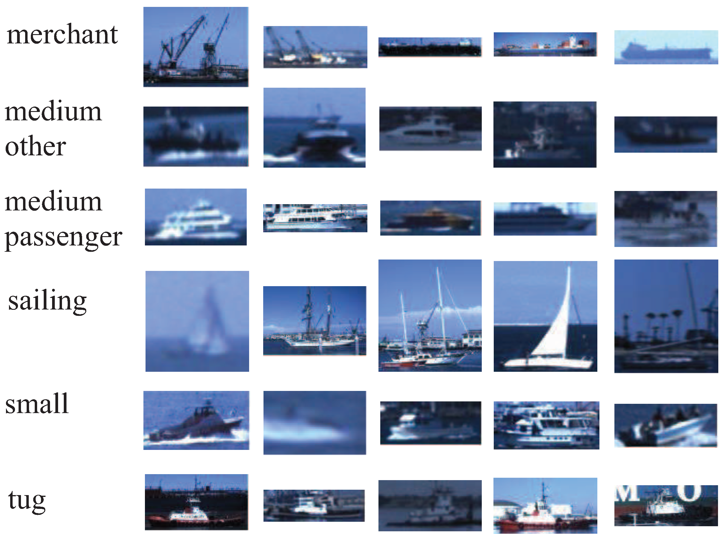
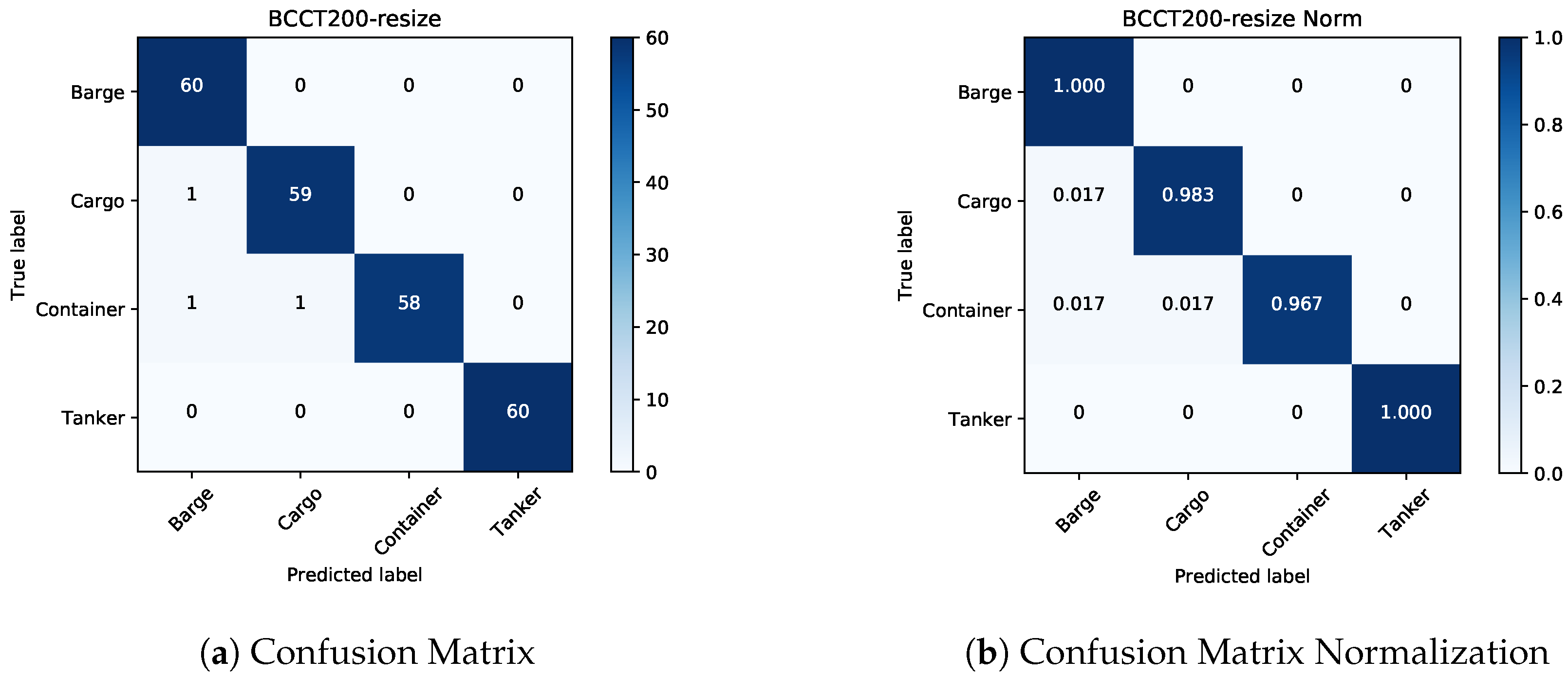
Section 3 reports the experimental results and analyses on the experimental datasets (i.e., BCCT200-resize [33] and VAIS [34]). Section 4 makes concluding remarks.

2. Proposed Ship Classification Method

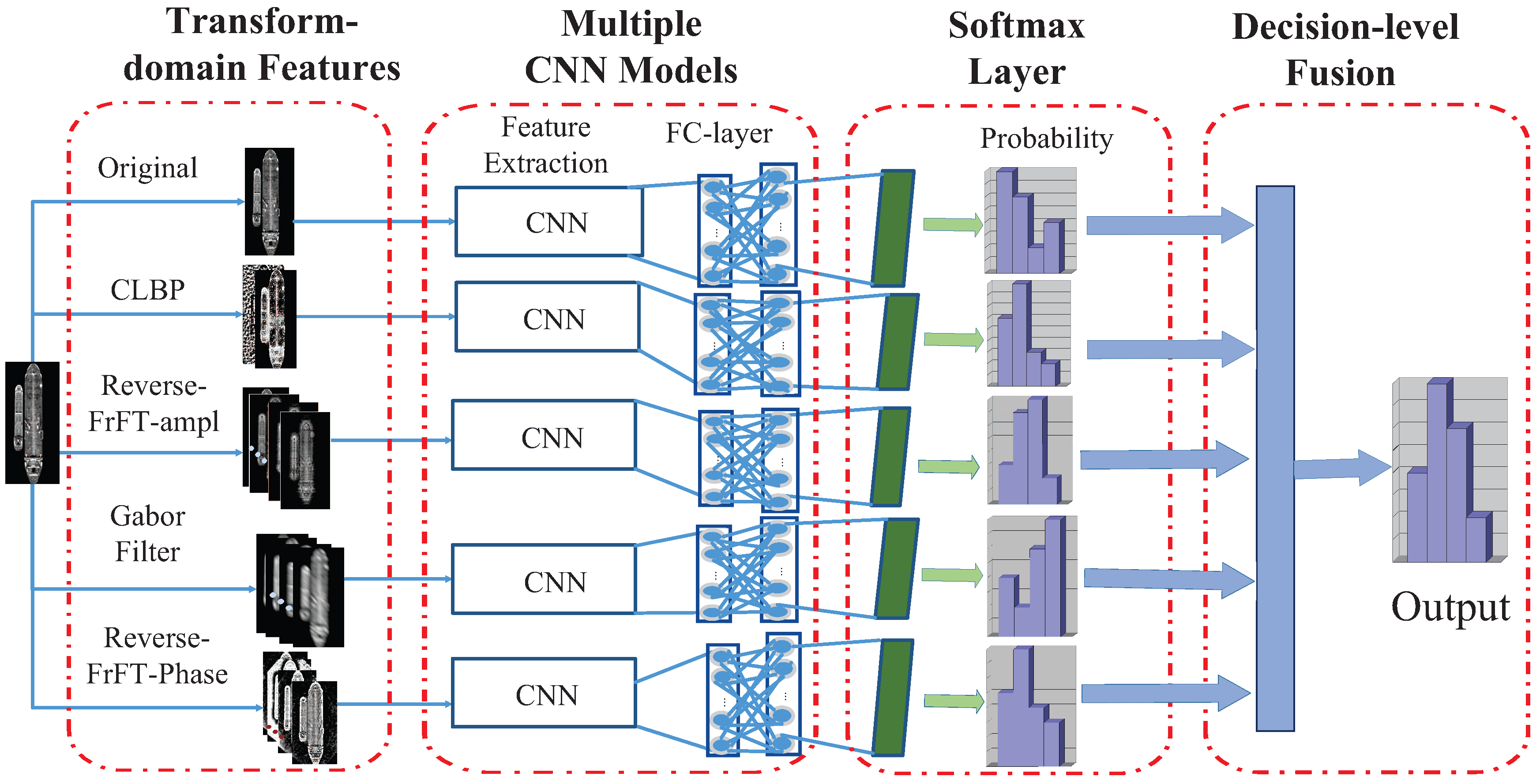
The task of the current work is to design a framework consisting of CNN and multifeatures for ship classification using optical remote sensing images. The flowchart of the proposed method is shown in Figure 1, which consists of four parts. In the first part, we extract the multifeatures that are viewed as the input of CNN. In the second part, CNN is used to learn the high-level features based on the image information mentioned above. To reduce network complexity, the network structure of each branch is the same. The probability of each branch can be obtained from the SoftMax layer of CNN in the third part. In the last part, the proposed method merges the outputs of each individual classification pipeline using decision-level soft fusion (i.e., logarithmic opinion pools (LOGP)) to gain the final classification result.

2.1. 2D Discrete Fractional Fourier Transformation

For the FrFT, the normalization of the data can reduce computational complexity, which makes the research process more convenient and effective. In this paper, we first normalize the image before the FrFT. Let f ( h , k ) be the ship image with the size of M × N . The formula is as follows:
M a x _ value = max max f h , k , f ( h , k ) = f h , k . / M a x _ value
where M a x _ value is maximum value of the sample image. Regarding deep learning, normalization can accelerate the speed of finding the optimal solution when the gradient descends, and improve classification accuracy. Thus, we take absolute values of amplitude and phase after inverse transformation, normalize them, and then put them into CNN for training.
To deal with the two-dimensional imagery and increase the speed of calculation, two-dimensional fractional Fourier transform (2D-FrFT) [20,35] is adopted. Compared with convolutional 2D discrete Fourier transform (DFT), 2D-DFrFT is more suitable and flexible with various orders. With the changing of rotation angle, the time-frequency domain characteristics of a transformed image are varied. For normalized images f ( h , k ) with the size of M × N , the 2D-DFrFT is calculated by the following equations:
F p 1 , p 2 u , v = 1 1 M N M N h = 1 M k = 1 N f ( h , k ) K p 1 , p 2 h , k ; u , v ,
with the kernel:
K p 1 , p 2 h , k ; u , v = K p 1 h , u K p 2 k , v ,
the K p 1 h , u is defined as:
K p 1 h , u = A ϕ h e x p j π h 2 cot ϕ h 2 h u csc ϕ h + u 2 cot ϕ h , ϕ h n π δ h u , ϕ h = 2 n π δ h + u , ϕ h = 2 n ± 1 π
where p 1 is the order, ϕ h = p 1 π p 1 π 2 2 is the rotation angle. Moreover, K p 1 h , u and K p 2 k , v have a similar form. Both are set as the same value, p 1 = p 2 = p , where p is the order of 2D-DFrFT, which is a significant parameter for vessel classification. Based on the above equation, it is obvious that the period of the transform kernel p is 4. Thus, any real value in range 0 , 4 can be selected for p. Specifically, FrFT is equivalent to the conventional FT when p 1 = p 2 = π π 2 2 . Because fractional transformation itself has periodicity and the symmetry property, we only need to study the transformation order value in the range 0 , 1 .
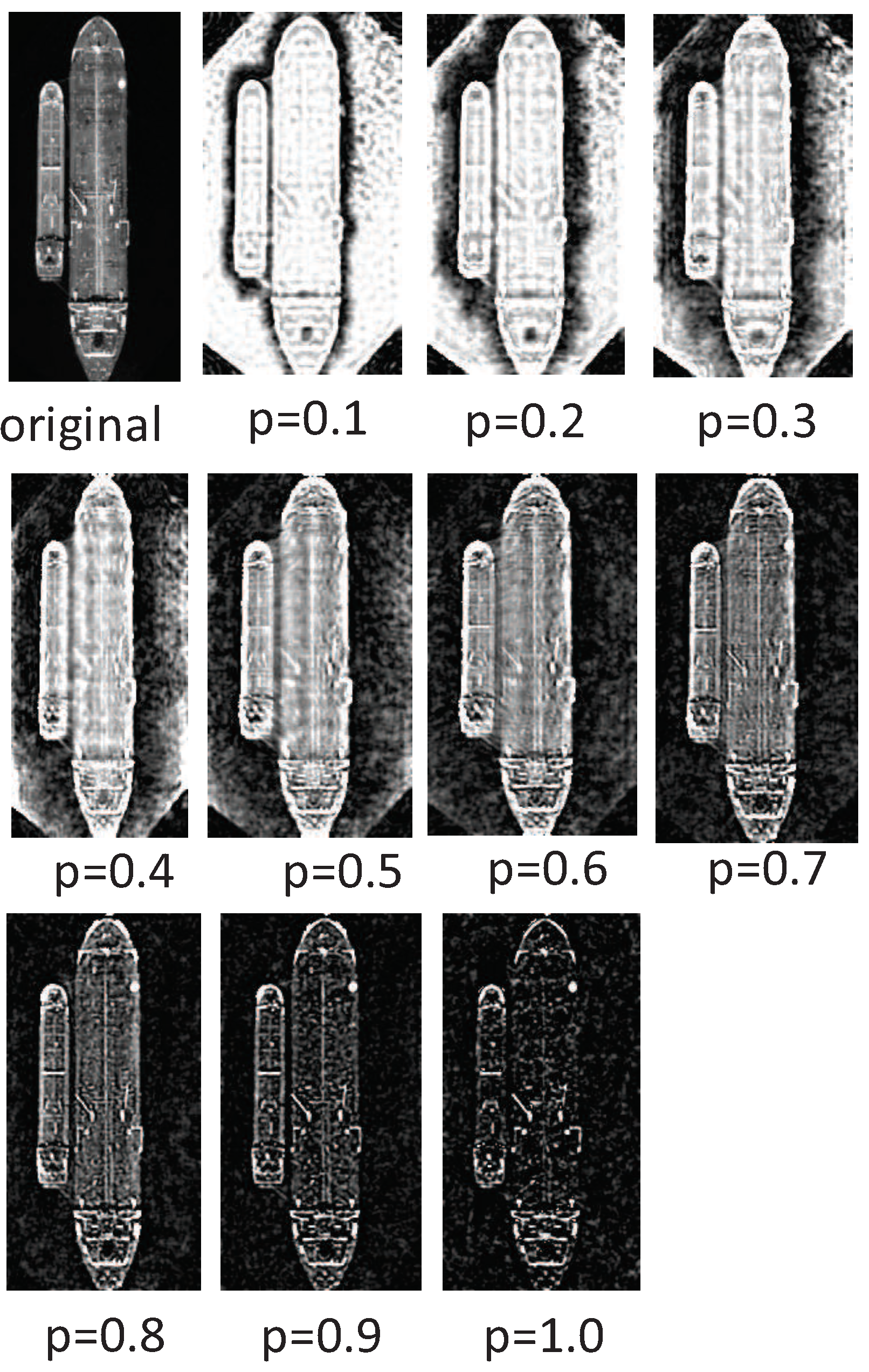
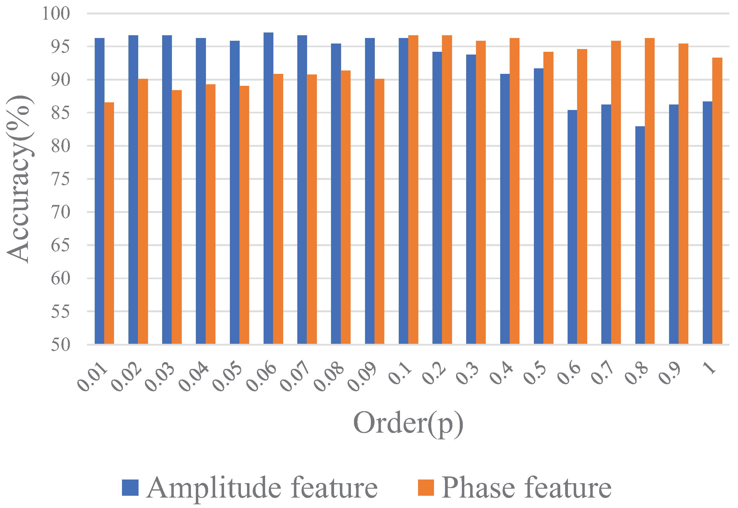
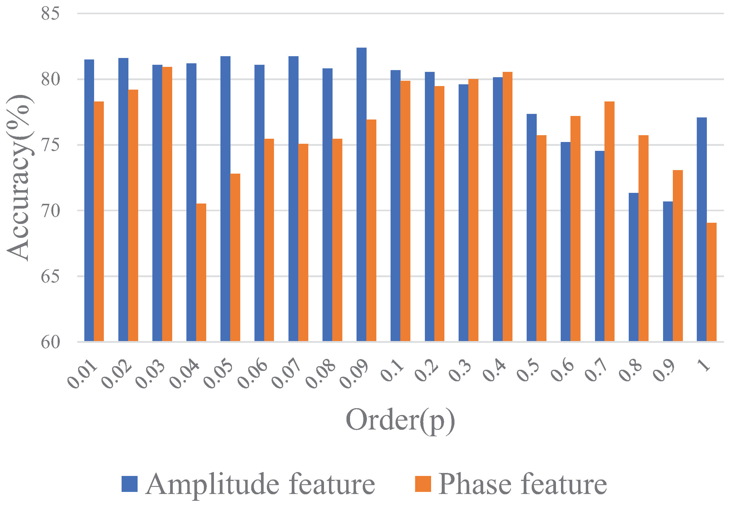
Given the aforementioned brief description of the 2D-DFrFT, there are some difficulties in analyzing the amplitude and phase information of the fractional domain directly, because the amplitude and phase information of the fractional domain contain time-frequency domain information. Therefore, the next step of analysis is based on the amplitude and phase information after the fractional Fourier inverse transform is done. As shown in Figure 2 and Figure 3, it can be noticed that both amplitude and phase information contain some useful characteristics for contributing the improvement of the classification approach. Furthermore, it is easily found that amplitude information extracted from the inverse 2D-DFrFT mainly contains useful information such as profile, texture, etc., especially small details; in addition, with the gradual increase of order, the energy of the image becomes more concentrated. The phase information obtained from the inverse 2D-DFrFT mainly consists of edges, profile information. In addition, various 2D-DFrFT order amplitude features can reflect different characteristics of the original ship image. Therefore, combining multi-order 2D-DFrFT features can achieve better classification performance compared with using only single 2D-DFrFT features.

2.2. Reverse 2D-DFrFT on Amplitude Image

For each ship image, it is first handled by 2D-DFrFT, according to the above-mentioned details, to get amplitude and phase information. As shown in Figure 1, the amplitude of the inverse 2D-DFrFT is calculated according to amplitude value in the fractional domain. For the ship image f ( h , k ) , F T 2 D represents 2D-DFrFT operator, and the amplitude information A P ( u , v ) is obtained as follows:
F u , v = F T 2 D f ( h , k ) ) ,
A P u , v = F u , v .
The inverse 2D-DFrFT of amplitude is the 2D-DFrFT with order p . Specifically, assuming a p ( h , k ) represents the amplitude information of the ship image in fractional domain transformed by inverse 2D-DFrFT, F T 2 D is the inverse 2D-DFrFT operator:
a p h , k = F T 2 D A P u , v .
The amplitude information of Equation (7) is one of the multifeature inputs of the third CNN pipeline.

2.3. Reverse 2D-DFrFT on Phase Image

The phase of the inverse 2D-DFrFT is calculated based on phase information in the fractional domain. The calculation process is very similar to the amplitude, that is, the phase information P P ( u , v ) of 2D-DFrFT is defined,
P P u , v = F u , v P P u , v = F u , v A P u , v .
Assuming p p ( h , k ) represent the phase information of inverse 2D-DFrFT,
p p h , k = F T 2 D P P u , v .
The phase information of Equation (9) is the feature used in the last branch. However, compared with the original data, the phase image of the inverse 2D-DFrFT tends to contain a lot of noise. To obtain better classification results, a simple low-pass Gaussian filter is employed to remove noise, and then it is fed into CNN.
2D-DFrFT, as above-mentioned in detail, is employed to acquire amplitude and phase information. Then both, after inverse 2D-DFrFT, are fed into CNN to obtain more abstract feature representation. As described in Algorithm 1, the training set is first prepared well; then, the phase and amplitude information are obtained by 2D-DFrFT. To reduce the complexity of research, we use the inverse transform information, which is calculated by inverse 2D-DFrFT. Since the inverse transform information is still a complex value, we only take its absolute value to study, and because the phase information contains noise, the filtering operation is performed.
Algorithm 1 Amplitude and phase information extraction
Require: Prepared training set and testing set
1:
Each ship image is normalized and transformed by using 2D-DFrFT filter to obtain amplitude pictures (AP) and phase pictures (PP) in fractional domain.
2:
AP and PP are handled using inverse 2D-DFrFT.
3:
The absolute value of AP and PP after inverting is obtained.
4:
This information after inversion is normalized.
5:
For PP, because it contains noise, Gaussian filter is adopted to obtain better features.
Ensure: AP and PP in time domain

2.4. Gabor Filter and CLBP

A Gabor filter has good characteristics to extract directional features and enhance the global rotation invariance, which has been applied in face recognition [36] and scene classification [37].
It is defined as follows:
G ( c , d ; λ , θ , σ , γ , ψ ) = exp ( c 0 2 + γ 2 d 0 2 2 σ 2 ) · ( cos ( 2 π c 0 λ + ψ ) + j sin ( 2 π c 0 λ + ψ ) )
c 0 = c cos θ + d sin θ d 0 = c sin θ + d cos θ
where c and d are the location of the pixels in the space, γ is the aspect ratio that determines the ellipticity of the Gabor function (its value is 0.5), λ is the wavelength (note that its value is usually greater than or equal to 2 but less than 1 / 5 of the input image), b w is the bandwidth, ψ is the phase offset (its value range is from −180 to 180 degrees), and θ is the direction that regulates the direction of the parallel stripes when the Gabor function processes the image, taking values between 0 and 360 degrees.
A LBP descriptor has been applied in vessel recognition. However, it is not perfect and still needs to be improved. Based on this, CLBP was proposed to overcome the shortcoming of LBP, which mainly includes sign and magnitude information and has the advantages of lower computational complexity and high distinctiveness. It mainly contains two kinds of descriptive operators, such as CLBP_Sign (CLBP_S), CLBP_Magnitude (CLBP_M). Both are complementary to one another. The definition is expressed as follows:
C L B P _ M m , R = i = 0 m 1 U ( Q i D ) 2 i
C L B P _ S m , R = i = 0 m 1 U ( s i s c ) 2 i
U ( s i s c ) = 0 , i f s i < s c 1 , i f s i > s c
D = 1 L l = 0 L 1 1 m i = 0 m 1 ( s i s c )
where R is the distance from the center point, and m is the number of nearest neighbors, s i represents the gray value of the neighbors, Q i = s i s c , and L is the number of sub-windows for image partition. Here, CLBP_S is the same as the traditional LBP definition. CLBP_M compares the difference between the grayscale amplitude of two pixels and the global grayscale and describes the gradient difference information of the local window, which reflects the contrast.

2.5. Convolutional Neural Network

Based on the multifeatures ensemble, CNN is further employed for feature extraction. A normal CNN consists of several layers: convolutional layers to learn hierarchy local features; pooling layers to reduce the dimension of the feature maps; activation layers to produce non-linearity; dropout layers to avoid the problem of over-fitting; fully connected layers to use the global feature and SoftMax layers to predict the category probability. Here, the cross-entropy loss formula is defined as:
J a = i i = 1 M M log e W y i i T x i i + b y i i j j = 1 N N e W j j T x + b j j ,
where x i i is the i i th feature, y i i is the target class, M M is the batch size, N N is the number of the category, and W is the weight matrix of the fully connected layer and b is the bias.
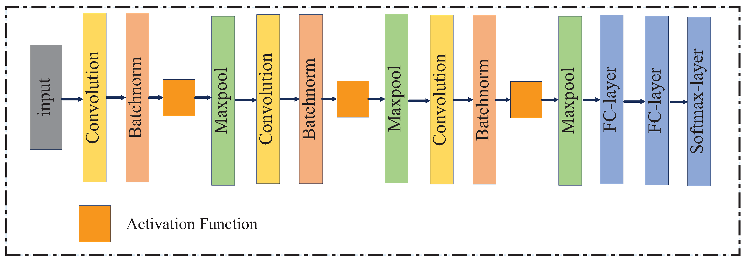
In the proposed framework, based on AlextNet, we have made some changes to the network structure. Firstly, because each feature image is composed of multiple channels as the input of CNN, which increases the number of datasets in a sense, we choose to start the training network from scratch instead of using the fine-tuning strategy. Considering the performance and computational complexity, we reduce the number of convolution layers from five to three. Secondly, Batchnorm layer [38] is added to the network, which can reduce the absolute difference between images, highlight relative differences, and accelerate training speed. Furthermore, a strategy, i.e., local response normalization, LRN, is adopted to improve the performance of the framework and accelerate the training speed of the network. The dropout layer is employed in the last two fully connected layers to avoid the problem of over-fitting and improve the generalization ability of the network. Here, the drop parameter is set 0.75. The further parameters of the designed CNN are listed in Table 1 and the detailed structure is shown in Figure 4.
Finally, since multifeatures can reflect different information about the original image, and to obtain better classification accuracy, integration strategies, i.e., decision-level fusion, are adopted. Soft LOGP [16,39] is employed to combine the posterior probability estimations provided from each individual classification pipeline. The process further improves the performance of a single classifier that uses a certain type of feature.

2.6. Decision-Level Fusion

Decision-level fusion merges results from different classification pipelines and combines distinct classification results into a final decision, which can show better performance than a single classifier using an individual feature. As a special case of decision-level fusion, score-level fusion is equivalent to soft fusion. The aim is to combine the posterior probability estimations provided from each single classifier by using score-level fusion. In this work, the soft LOGP is employed to obtain the result.
The LOGP [16,39] takes advantage of conditional class probability from the individual classification pipeline to estimate a global membership function P r q | t . Assume r is a final class label, which can be given according to:
r = arg max q = 1 , 2 , , Q = P r q | t ,
where Q is the number of classes, and r q indicates the qth class belong to which one in a sample t. The global membership function is as follows:
P r q | t = z = 1 Z p z r q | t α z ,
or
l o g P r q | t = z = 1 Z α z p z r q | t
where p z r q | t represents the conditional class probability of the z classifier, α z z = 1 Z is the classifier weights uniformly distributed over all of classifiers, and Z is number classifiers.

2.7. Motivation of Proposed Method

The motivation of developing a ME-CNN to learn image characteristics for ship classification is as follows: firstly, for Gabor filter, which is rotation-invariant and orientation-sensitive; i.e., it can extract the global features in different directions for images. In terms of ship recognition, this characteristic is very important, because different orientations of the bow lead to greater intra-class differences, which may affect the classification results. For CNN, it can only obtain local rotation invariance features by pooling operations, but it is more important for ship recognition with global rotation invariance. Therefore, it is meaningful to combine Gabor filter with CNN for ship recognition.
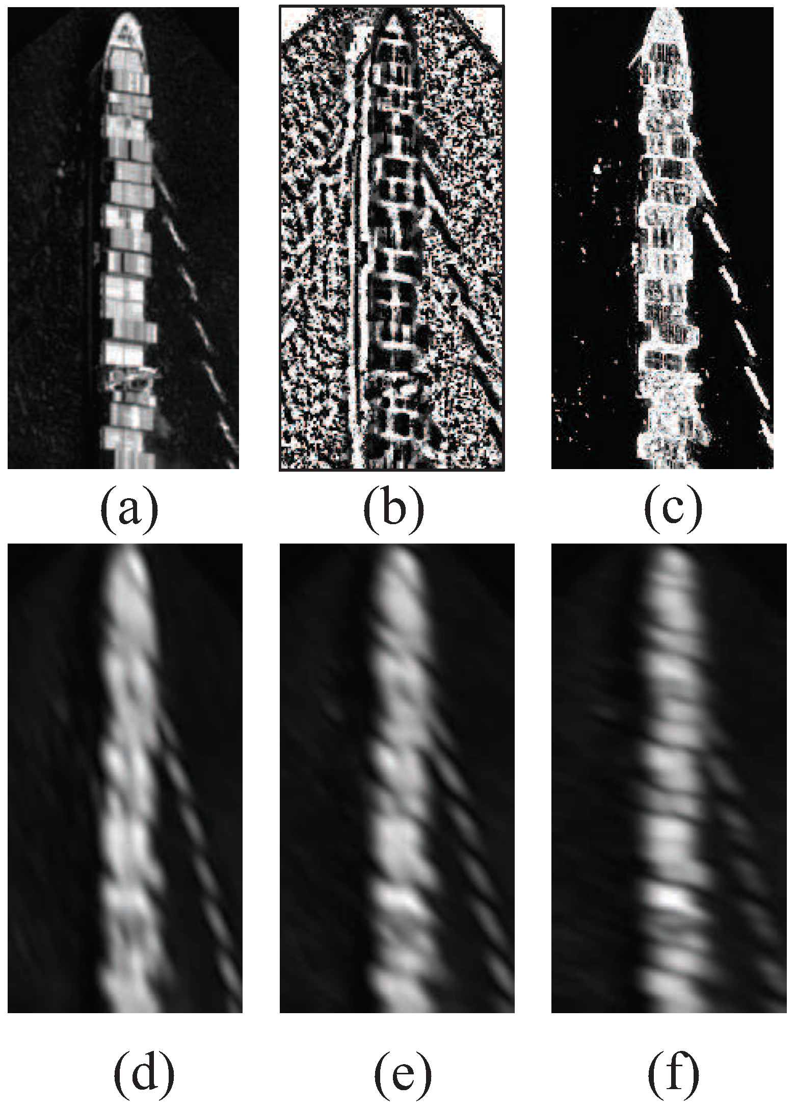
Secondly, because the categories of ship are various, this may cause the structure features to be more complex and changeable; thus, the local texture, edge, and profile information are expected; however, CNN cannot extract all low-level features based on the raw data. CLBP descriptor, as a local texture feature descriptor, captures the spatial information of the original image and extracts the local texture features, and has two descriptor operators CLBP_S and CLBP_M. CLBP_M extracts more contour information of the ship image, while CLBP_S extracts more detailed features of local texture of ship image. Therefore, the obtained features have stronger robustness. The Gabor filter and CLBP images are shown in Figure 5.
Thirdly, 2D-DFrFT, as a generalized form of Fourier transform, has the advantages of Fourier transform and has its own unique characteristics. As shown in Figure 2 and Figure 3, 2D-DFrFT features of various orders extracted from the same image usually reflect different characteristics of the original image. Therefore, the combination of multi-order various features is important, which makes the feature representation more discriminative. Furthermore, it has been viewed as a vital tool for handling chirp signals, which can capture the profile and detailed formation. The ship image can be regarded as a gradually changing signal and has some similarity to a face image. Thus, inspired by this advantage of 2D-DFrFT, we use it to extract amplitude and phase information. Although the features mentioned above have their own advantages, they do not have all the characteristics of ship identification, and they are complementary. Therefore, it is necessary to form multifeatures, which combine their respective advantages, making the features richer and more separable.
Finally, the reason that CNN is chosen to continue to learn high-level features based on the features mentioned above is that the network has the capacity to capture structure information automatically by layer-to-layer propagation. Compared with low-level features, these are more abstract, robust, and discriminative for dealing with within-class differences and inter-class similarity.

3. Experiments and Analysis

In this section, extensive experiments are conducted to evaluate the effectiveness of the proposed approach by using optical remote sensing imagery. All the experiments are conducted in Python, MATLAB, and Caffe. The Caffe is a deep learning tool developed by the Berkeley vision and community contributors [40]. The experimental environment is Ubuntu 14.04, dual Intel i5 4590 CPUs, 8GB memory, and GPU of Nvidia GTX 970.

3.1. Experimental Datasets

The first available dataset is called BCCT200-resize [33], and consists of small grayscale ship images that have been chipped out of larger electro-optical satellite images by the RAPIER Ship Detection System. They were rotated and aligned to have uniform dimensions and orientation in the procedure of preprocessing, including 4 ship categories, i.e., barge ships, cargo ships, container ships, and tanker ships, and each type of ship target has 200 images comprising 300 × 150 pixels, as illustrated in Figure 6. More detailed information of the training and testing samples is listed in Table 2.
The second dataset is the original BCCT200 dataset, which also consists of small grayscale ship images chipped out of larger electro-optical satellite images by the RAPIER Ship Detection System. However, in contrast to the first dataset, they are unprocessed, and at various orientations and resolutions, which makes the data more challenging. The data includes four classes: barges, cargo ships, container ships, and tankers, and 200 images per class, as shown in Figure 7. To achieve a fair comparison, we follow the same experimental setup illustrated in [13] for the above two datasets. To obtain the available data for the proposed approach, a cross-validation strategy is adopted during the process. The number of the training and testing samples is shown in Table 3.
The third data is the world’s first publicly available data, referred to as VAIS, which consists of paired visible and infrared ship images [34]. The dataset includes 2865 images (1623 visible and 1242 infrared), of which there are 1088 corresponding pairs in total. It has 6 coarse-grained categories, i.e., merchant ships, sailing ships, medium-passenger ships, medium “other” ships, tug boats, and small boats. The area of the visible bounding boxes ranges from 644 to 6,350,890 pixels, with a mean of 181,319 pixels and a median of 13,064 pixels, as shown in Figure 8.
The dataset is partitioned into “official” train and test groups. Specifically, it makes 539 image pairs and 334 singletons for training, and 549 image pairs and 358 singletons for testing. In this paper, we only conduct experiments based on the visible ship imagery category. To facilitate a fair comparison, before 2D-DFrFT, we resize each ship image to size 256 × 256 using bicubic interpolation, which is implemented the same as [34], and the number of training and testing samples is illustrated in Table 4.

3.2. Parameters Setting

The detailed architecture is shown in Table 1. In the proposed classification framework, 8 orientations of Gabor filters are selected, and the spatial frequency bandwidth is set at 5 for all the experimental data. After that, the 8 Gabor images of each sample are composed of multiple channels of the inputs of CNN. That is to say, for Gabor feature images, the CNN architecture includes 8 input maps with size 256 × 256 . The operation of CLBP feature images is similar. For 2D-DFrFT, to test the influence on classification, different orders are selected to process ship images using 2D-DFrFT with the interval of 0.01 in the range of 0 , 1 . Various orders have different contributions to feature extraction, so we discuss the effect of parameter p for 2D-DFrFT. Based on Figure 9, Figure 10 and Figure 11, it is easy to discover that the amplitude information shows excellent performance at 0.01, 0.02, and 0.03, so we have reason to believe that the amplitude of these three orders contain more useful information than other orders. Similarly, it can be observed that phase information achieves better results at 0.1, 0.2, and 0.3. That is to say, compared with other orders, they contain more important information. comprehensively considering the computational performance and classification effect, for the three datasets, we use the amplitude and phase of three orders to form multi-channel images as the input of CNN.
During the processing, we unify the size of the experimental image to 256 × 256 , and then the output image, i.e., amplitude and phase value, of the 2D-DFrFT is cut from the four corners and centers of it to obtain subregions of the same size 227 × 227 as the input of the CNN. Experimental results demonstrate that the operation is helpful for training the network, mainly because it can increase the amount of training data so it will not produce a bad influence on training, but largely avoid over-fitting. Finally, a 4096-dimensional feature vector of the second fully connected layer is obtained.
As for CNN, and some parameters are important. Specifically, for the BCCT200-resize data, the learning rate is set as 0.0001 with the policy of Adam [41]. The momentum is 0.9, gamma is 0.95, weight decay is 0.001, and the max iteration is 30000. As for the original BCCT200 data, the learning rate is set as 0.00001 with the policy of Adam [41]. The momentum is 0.99, gamma is 0.95, weight decay is 0.004, and the max iteration is 30,000. As for the VAIS data, the learning rate is set as 0.00001 with the policy of Adam [41]. The momentum is 0.99, gamma is 0.9, weight decay is 0.1, and the max iteration is 30,000.

3.3. Classification Performance and Analysis

As listed in Table 5, we find that the filtering operation on phase information is effective. Therefore, it is also implemented in another two datasets. To verify the effectiveness of the proposed method, we compare it with other state-of-the-art algorithms, and the results are reported in Table 5, Table 6 and Table 7 for three experimental datasets. All methods are conducted on the same image set. Specifically, 2D-DFrFT-M and 2D-DFrFT-P are the representation of amplitude (M) and phase (P) information after inverse transformation, respectively [21]. Obviously, the proposed algorithm outperforms other existing methods, which demonstrates the effectiveness of the proposed framework for ship classification. Specifically, for the BCCT200-resize dataset, the proposed classifier performs with an accuracy of 98.75%, while the hierarchical multi-scale LBP (HMLBP) obtained an accuracy of 90.80%, with an improvement of approximate 8%; compared with the state-of-art MFL, the improvement is about 4%. For the original BCCT200 dataset, the proposed method gains about 5% overall accuracy compared with the MFL algorithm [13]. Moreover, for the VAIS dataset, the improvement of the proposed approach compared with the MFL is 2%. Therefore, the proposed method, which combines multiple features by decision-level fusion strategy, has obvious advantages. The reason is that the method proposed in this paper combines the advantages of several features that are beneficial for ship classification. Specifically, the Gabor filter can acquire the global rotation invariance feature of the ship, which is especially important for vessel identification. CLBP can extract texture information of the ship, etc. 2D-DFrFT can obtain the edge and profile information of the ship, etc. Based on these characteristics, CNN can learn more abstract and specific features better, but these features do not have all the advantages required for ship classification, so a fusion strategy is adopted to obtain more abundant and discriminative features, thus achieving better performance.
Furthermore, for the BCCT200-resize dataset, the proposed approach yields the highest classification accuracy of 98.75%, and the 2D-DFrFT-P+CNN obtains an accuracy of 95.00%, with an improvement of approximately 5%. For the original BCCT200 dataset, the improvement is about 16% compared with the 2D-DFrFT-P+CNN. For the VAIS dataset, the improvement is also obvious. This can be explained because the classic ship feature extraction approach misjudged the non-ship region to be ship area and part of information is lost. On the contrary, the proposed method not only adopts CNN to effectively capture the high-level features, but also takes full advantage of the complementary information of 2D-DFrFT to extract features, and the global feature of Gabor filter and local feature of CLBP, which enhances discriminative information.
To validate the enhanced discriminative power of the proposed approach, we compare the classification accuracy of the proposed multiple CNN fusion strategy with the performance of the methods that use each individual feature in the classification framework. The experimental results are listed in Table 8, Table 9 and Table 10. Obviously, the proposed method shows better performance than all the other approaches based on the individual features. Specifically, for the BCCT200-resize data, the global feature representation method, i.e., 2D-DFrFT-M+CNN, achieves maximum accuracy for the container category. For the VAIS data, 2D-DFrFT-M+CNN, gains highest accuracy for medium-passenger category, while Gabor+CNN obtains better performance for medium-other categories. Nevertheless, the proposed classification framework achieves superior performance for other classes and the highest overall accuracy for three experimental datasets.
Figure 12 depicts the confusion matrix of the proposed method with decision-level fusion strategy for the BCCT200-resize dataset. It is obvious that the major confusion occurs between class 1 (i.e., barge) and class 3 (i.e., container), since some barge images are similar to the container images. Figure 13 displays the confusion matrix of the proposed method for the original BCCT200 dataset. It is easily found that major confusion occurs between class 2 (i.e., cargo) and class 4 (i.e., tanker), or between class 2 (i.e., cargo) and class 4 (i.e., container). Figure 14 shows the confusion matrix of the proposed approach for the VAIS dataset. It is observed that major confusion occurs within class 1 (i.e., merchant), class 2 (i.e., medium-other) and class 5 (i.e., small), or between class 3 (i.e., medium-passenger) and class 5 (i.e., small). The reason for this is that small ships include speedboats, jet-skis, smaller pleasure, and larger pleasure, medium-other ships include fishing, medium-other, and some small ships and medium-other ships have relatively high similarity. Furthermore, as shown in Figure 14, it is easily found that the medium-other and medium-passenger classifications have a lower accuracy. The reason is that the quality of this dataset is not very good, and some of the graphics are vague, especially ones of the categories in the medium-other category and the tour boat in the medium-passenger; the other is that some small images and medium-passenger exist similarity.
To validate the effectiveness of to the proposed method when the number of training datasets is varied, we also carried out an experiment. The results are listed in Table 11. Specifically, Train/Test set: [ 140 / 60 ] means that 140 images per category are considered for training and 60 images per category are viewed as testing. It is obvious that even with a small number of training sets, the classification performance of the proposed method is always better than that of other single-branch CNN under the uniform condition of training samples and test samples. Specifically, even if the training set is very small, (e.g., 40), the approach presented in this paper still shows excellent performance, which proves the effectiveness of the proposed framework.
The standardized McNemar’s test is usually employed in evaluating the statistical significance about the performance improvement of the proposed approach. When the Z value of McNemar’s test is larger than 1.96 and 2.58, it means that the two results are statistically different with the confidence level of 95% and 99%, respectively. The sign of Z denotes whether the first classifier outperforms the second classifier (Z > 0). In our experiments, the comparison between the proposed method and other individual methods is made separately. As listed in Table 12, all values are larger than 2.58, which demonstrates the effectiveness of the proposed approach.

4. Conclusions

In this paper, a novel classification framework (ME-CNN) was proposed for classifying category of ship. Inspired by the success of 2D-DFrFT in face recognition, we proposed to employ multi-order amplitude and phase images as the inputs of CNN, respectively. Furthermore, because Gabor filter and CLBP descriptor have been successfully applied in the field of face recognition and ship classification, the Gabor filter was used to obtain global rotation-invariant features to make up the shortcomings of CNN; CLBP was used to extract the local texture information, which is important for ship classification. All the above multifeatures were viewed as the input of deep CNN. Those features are complementary to each other and the combination of them is a powerful and comprehensive representation of ship images. It is easily found that the proposed approach has shown superior performance than the individual feature-based methods. Through experimental results, the proposed ME-CNN has provided excellent performance when compared to other state-of-the-art methods, which further demonstrates the effectiveness of the proposed classification framework.
Encouraged by the successful application of improved CNN, especially in the field of image recognition, future work should apply the improved method based on CNN directly to ship classification tasks.

Author Contributions

All authors conceived and designed the study. Q.S. carried out the experiments. All authors discussed the basic structure of the manuscript, and Q.S. finished the first draft. W.L., R.T., X.S. and L.G. reviewed and edited the draft.

Funding

This work is supported by National Key Research and Development Program of China (2016YFB0501501).

Acknowledgments

This work is supported by National Key Research and Development Program of China (2016YFB0501501).

Conflicts of Interest

The authors declare no conflict of interest.

References

  1. Kanjir, U.; Greidanus, H.; Oštir, K. Vessel detection and classification from spaceborne optical images: A literature survey. Remote Sens. Environ. 2018, 207, 1–26. [Google Scholar] [CrossRef] [PubMed]
  2. Leng, X.; Ji, K.; Zhou, S.; Xing, X.; Zou, H. An Adaptive Ship Detection Scheme for Spaceborne SAR Imagery. Sensors 2016, 16, 1345. [Google Scholar] [CrossRef] [PubMed]
  3. Park, S.; Cho, C.J.; Ku, B.; Lee, S.H.; Ko, H. Simulation and Ship Detection Using Surface Radial Current Observing Compact HF Radar. IEEE J. Ocean. Eng. 2016, 42, 544–555. [Google Scholar] [CrossRef]
  4. Huang, S.; Xu, H.; Xia, X. Active deep belief networks for ship recognition based on BvSB. Optik Int. J. Light Electron Opt. 2016, 127, 11688–11697. [Google Scholar] [CrossRef]
  5. Lu, H.; Plataniotis, K.N.; Venetsanopoulos, A.N. MPCA: Multilinear Principal Component Analysis of Tensor Objects. IEEE Trans. Neural Netw. 2008, 19, 18–39. [Google Scholar] [PubMed] [Green Version]
  6. Condurache, A.P.; Müller, F.; Mertins, A. An LDA-based Relative Hysteresis Classifier with Application to Segmentation of Retinal Vessels. In Proceedings of the International Conference on Pattern Recognition, Istanbul, Turkey, 23–26 August 2010; pp. 4202–4205. [Google Scholar]
  7. Guo, Z.; Zhang, L.; Zhang, D.; Mou, X. Hierarchical multiscale LBP for face and palmprint recognition. In Proceedings of the IEEE International Conference on Image Processing, Hong Kong, China, 26–29 September 2010; pp. 4521–4524. [Google Scholar]
  8. Rybski, P.E.; Huber, D.; Morris, D.D.; Hoffman, R. Visual classification of coarse vehicle orientation using Histogram of Oriented Gradients features. In Proceedings of the Intelligent Vehicles Symposium, San Diego, CA, USA, 21–24 June 2010; pp. 921–928. [Google Scholar]
  9. Parameswaran, S.; Rainey, K. Vessel classification in overhead satellite imagery using weighted “bag of visual words”. Proc. SPIE 2015, 9476, 947609. [Google Scholar] [CrossRef]
  10. Rainey, K.; Parameswaran, S.; Harguess, J.; Stastny, J. Vessel classification in overhead satellite imagery using learned dictionaries. Proc. SPIE 2012, 8499, 84992F. [Google Scholar]
  11. Arguedas, V.F. Texture-based vessel classifier for electro-optical satellite imagery. In Proceedings of the IEEE International Conference on Image Processing, Quebec City, QC, Canada, 27–30 September 2015; pp. 3866–3870. [Google Scholar]
  12. Zhenhua, G.; Lei, Z.; David, Z. A completed modeling of local binary pattern operator for texture classification. IEEE Trans. Image Process. 2010, 19, 1657–1663. [Google Scholar] [CrossRef] [PubMed]
  13. Huang, L.; Li, W.; Chen, C.; Zhang, F.; Lang, H. Multiple features learning for ship classification in optical imagery. Multimedia Tools Appl. 2018, 77, 13363–13389. [Google Scholar] [CrossRef]
  14. Huang, L.; Chen, C.; Li, W.; Du, Q. Remote Sensing Image Scene Classification Using Multi-Scale Completed Local Binary Patterns and Fisher Vectors. Remote Sens. 2016, 8, 483. [Google Scholar] [CrossRef]
  15. Cid, F.; Prado, J.A.; Bustos, P.; Núnez, P. A real time and robust facial expression recognition and imitation approach for affective human-robot interaction using Gabor filtering. In Proceedings of the IEEE International Conference on Intelligent Robots and Systems, Tokyo, Japan, 3–7 November 2013; pp. 2188–2193. [Google Scholar]
  16. Li, W.; Chen, C.; Su, H.; Du, Q. Local Binary Patterns and Extreme Learning Machine for Hyperspectral Imagery Classification. IEEE Trans. Geosci. Remote Sens. 2015, 53, 3681–3693. [Google Scholar] [CrossRef]
  17. Ozaktas, H.M.; Kutay, M.A. The fractional fourier transform. In Proceedings of the 2001 European Control Conference (ECC), Porto, Portugal, 4–7 September 2001; pp. 1477–1483. [Google Scholar]
  18. Sejdić, E.; Djurović, I.; Stanković, L. Fractional Fourier transform as a signal processing tool: An overview of recent developments. Signal Process. 2011, 91, 1351–1369. [Google Scholar] [CrossRef] [Green Version]
  19. Tao, R.; Deng, B.; Wang, Y. Research progress of the fractional Fourier transform in signal processing. Sci. China Ser. F 2006, 49, 1–25. [Google Scholar] [CrossRef]
  20. Liu, S.; Li, Y.; Zhu, B. Optical image encryption by cascaded fractional Fourier transforms with random phase filtering. Opt. Commun. 2001, 187, 57–63. [Google Scholar] [CrossRef]
  21. Wang, Y.; Qi, L.; Guo, X.; Gao, L. Face recognition based on histogram of the 2D-FrFT magnitude and phase. In Proceedings of the International Conference on Information Science, Electronics and Electrical Engineering, Sapporo, Japan, 26–28 April 2014; pp. 1421–1425. [Google Scholar]
  22. Gao, L.; Qi, L.; Chen, E.; Mu, X.; Guan, L. Recognizing Human Emotional State Based on the Phase Information of the Two Dimensional Fractional Fourier Transform. In Proceedings of the Advances in Multimedia Information Processing, and Pacific Rim Conference on Multimedia, Shanghai, China, 22–24 September 2010; pp. 694–704. [Google Scholar]
  23. Jia, K.; Qi, L.; Gao, L.; Zheng, N. Recognizing facial expression based on discriminative multi-order Two Dimensions Fractional Fourier Transform. In Proceedings of the International Congress on Image and Signal Processing, Chongqing, China, 16–18 October 2012; pp. 469–473. [Google Scholar]
  24. Krizhevsky, A.; Sutskever, I.; Hinton, G.E. ImageNet classification with deep convolutional neural networks. In Proceedings of the International Conference on Neural Information Processing Systems, Lake Tahoe, NV, USA, 3–6 December 2012; pp. 1097–1105. [Google Scholar]
  25. Schwarz, M.; Schulz, H.; Behnke, S. RGB-D object recognition and pose estimation based on pre-trained convolutional neural network features. In Proceedings of the IEEE International Conference on Robotics and Automation, Seattle, WA, USA, 26–30 May 2017; pp. 1329–1335. [Google Scholar]
  26. Kang, M.; Ji, K.; Leng, X.; Lin, Z. Contextual region-based convolutional neural network with multilayer fusion for SAR ship detection. Remote Sens. 2017, 9, 860. [Google Scholar] [CrossRef]
  27. Szegedy, C.; Liu, W.; Jia, Y.; Sermanet, P.; Reed, S.; Anguelov, D.; Erhan, D.; Vanhoucke, V.; Rabinovich, A. Going deeper with convolutions. In Proceedings of the IEEE Conference on Computer Vision and Pattern Recognition, Boston, MA, USA, 7–12 June 2015; pp. 1–9. [Google Scholar]
  28. Chung, J.; Sohn, K. Image-Based Learning to Measure Traffic Density Using a Deep Convolutional Neural Network. IEEE Trans. Intell. Transp. Syst. 2018, 19, 1670–1675. [Google Scholar] [CrossRef]
  29. He, K.; Zhang, X.; Ren, S.; Sun, J. Spatial Pyramid Pooling in Deep Convolutional Networks for Visual Recognition. IEEE Trans. Pattern Anal. Mach. Intell. 2015, 37, 1904–1916. [Google Scholar] [CrossRef] [PubMed]
  30. Rainey, K.; Reeder, J.D.; Corelli, A.G. Convolution neural networks for ship type recognition. In Automatic Target Recognition XXVI; International Society for Optics and Photonics: Baltimore, MA, USA, 2016; p. 984409. [Google Scholar] [CrossRef]
  31. Wang, Q.; Zheng, Y.; Yang, G.; Jin, W.; Chen, X.; Yin, Y. Multi-Scale Rotation-Invariant Convolutional Neural Networks for Lung Texture Classification. IEEE J. Biomed. Health Inform. 2017, 22, 184–195. [Google Scholar] [CrossRef] [PubMed]
  32. Gong, C.; Zhou, P.; Han, J. RIFD-CNN: Rotation-Invariant and Fisher Discriminative Convolutional Neural Networks for Object Detection. In Proceedings of the Computer Vision & Pattern Recognition, Las Vegas, NV, USA, 26 June–1 July 2016; pp. 2884–2893. [Google Scholar]
  33. Rainey, K.; Stastny, J. Object recognition in ocean imagery using feature selection and compressive sensing. In Proceedings of the IEEE Applied Imagery Pattern Recognition Workshop, Washington, DC, USA, 11–13 October 2011; pp. 1–6. [Google Scholar]
  34. Zhang, M.M.; Choi, J.; Daniilidis, K.; Wolf, M.T.; Kanan, C. VAIS: A dataset for recognizing maritime imagery in the visible and infrared spectrums. In Proceedings of the IEEE Conference on Computer Vision and Pattern Recognition Workshops, Boston, MA, USA, 7–12 June 2015; pp. 10–16. [Google Scholar]
  35. Shi, Q.; Li, W.; Tao, R. 2D-DFrFT Based Deep Network for Ship Classification in Remote Sensing Imagery. In Proceedings of the 2018 10th IAPR Workshop on Pattern Recognition in Remote Sensing (PRRS), Beijing, China, 19–20 August 2018; pp. 1–5. [Google Scholar]
  36. Bankar, P.V.; Pise, A.C. Face Recognition by using GABOR and LBP. In Proceedings of the 2015 International Conference on Communications and Signal Processing (ICCSP), Chengdu, China, 10–11 October 2015; pp. 0045–0048. [Google Scholar]
  37. Chen, C.; Zhou, L.; Guo, J.; Li, W.; Su, H.; Guo, F. Gabor-filtering-based completed local binary patterns for land-use scene classification. In Proceedings of the 2015 IEEE International Conference on Multimedia Big Data (BigMM), Beijing, China, 20–22 April 2015; pp. 324–329. [Google Scholar]
  38. Ioffe, S.; Szegedy, C. Batch Normalization: Accelerating Deep Network Training by Reducing Internal Covariate Shift. arXiv, 2015; arXiv:1502.03167. [Google Scholar]
  39. Li, W.; Prasad, S.; Fowler, J.E. Decision Fusion in Kernel-Induced Spaces for Hyperspectral Image Classification. IEEE Trans. Geosci. Remote Sens. 2014, 52, 3399–3411. [Google Scholar] [CrossRef] [Green Version]
  40. Jia, Y.; Shelhamer, E.; Donahue, J.; Karayev, S.; Long, J.; Girshick, R.; Guadarrama, S.; Darrell, T. Caffe: Convolutional architecture for fast feature embedding. In Proceedings of the 22nd ACM International Conference on Multimedia, Orlando, FL, USA, 3–7 November 2014; ACM: New York, NY, USA, 2014; pp. 675–678. [Google Scholar]
  41. Kingma, D.; Ba, J. Adam: A Method for Stochastic Optimization. arXiv, 2014; arXiv:1412.6980. [Google Scholar]
  42. Verbancsics, P.; Harguess, J. Image Classification Using Generative Neuro Evolution for Deep Learning. In Proceedings of the IEEE Winter Conference on Applications of Computer Vision, Waikoloa, HI, USA, 5–9 January 2015; pp. 488–493. [Google Scholar]
  43. Verbancsics, P.; Harguess, J. Feature Learning HyperNEAT: Evolving Neural Networks to Extract Features for Classification of Maritime Satellite Imagery. In Proceedings of the International Conference on Information Processing in Cells and Tissues, San Diego, CA, USA, 14–16 September 2015; pp. 208–220. [Google Scholar]
Figure 1. A flowchart of proposed classification framework in optical remote sensing imagery.
Remotesensing 11 00419 g001
Figure 2. The inverse 2D-DFrFT amplitude information corresponding to different orders.
Remotesensing 11 00419 g002
Figure 3. The inverse 2D-DFrFT phase information corresponding to different orders.
Remotesensing 11 00419 g003
Figure 4. Detailed structure display of CNN.
Remotesensing 11 00419 g004
Figure 5. Display of Gabor filter and CLBP images. (a) original image. (b) CLBP_S coded image. (c) CLBP_M coded image. (df) represent filtered images obtained by using Gabor filter with different orientations.
Remotesensing 11 00419 g005
Figure 6. Illustration of the BCCT200-resize data.
Remotesensing 11 00419 g006
Figure 7. Illustration of the original BCCT200 data.
Remotesensing 11 00419 g007
Figure 8. Illustration of the VAIS data.
Remotesensing 11 00419 g008
Figure 9. Classification results of Amplitude and Phase features under different orders using the BCCT200-resize data.
Remotesensing 11 00419 g009
Figure 10. Classification results of Amplitude and Phase features under different orders using the original BCCT200 data.
Remotesensing 11 00419 g010
Figure 11. Classification results of Amplitude and Phase features under different orders using VAIS data.
Remotesensing 11 00419 g011
Figure 12. Classification confusion matrix of the proposed ME-CNN using the BCCT200-resize data.
Remotesensing 11 00419 g012
Figure 13. Classification confusion matrix of the proposed ME-CNN using the original BCCT200 data.
Remotesensing 11 00419 g013
Figure 14. Classification confusion matrix of the proposed ME-CNN using the VAIS data.
Remotesensing 11 00419 g014
Table 1. The details of the designed CNN structure.
Layer.TypeKernel SizeFilter NumberStride
AConvolution11964
BBatchnorm---
CMaxPooling3-2
DConvolution53841
EBatchnorm---
FMaxPooling3-2
GConvolution33841
HBatchnorm---
JMaxPooling3-2
KFullyConnected4096--
LFullyConnected4096--
MSoftMax4--
Table 2. Selected classes for evaluation and the numbers of training and test set for the BCCT200-resize data.
No.ClassTrainTest
1Barge14060
2Cargo14060
3Container14060
4Tanker14060
Total560240
Table 3. Selected classes for evaluation and the numbers of training and testing set for the original BCCT200 data.
No.ClassTrainTest
1Barge16040
2Cargo16040
3Container16040
4Tanker16060
Total640160
Table 4. Selected classes for evaluation and the numbers of training and test samples using the VAIS data.
No.ClassTrainTest
1Merchant10371
2Medium-other9986
3Medium-Passenger7862
4Sailing214198
5Small342313
6Tug3720
Total873750
Table 5. Comparison of classification accuracy (%) with some state-of-the-art methods for the BCCT200-resize data.
MethodAccuracy (%)
MPCA + SVM [10]79.10
BOW + SVM [10]76.80
HOG + SVM [10]81.60
PCA + SVM [10]77.10
LDA + SVM [10]74.10
Hierarchical multi-scale LBP(HMLBP) [10]90.80
Gabor + MS-CLBP + SVM [13]90.63
Deep Learning HyperNEAT [42]83.70
MFL(decision-level) + ELM [13]94.63
MFL(decision-level) + SVM [13]94.63
CNN [30]96.25
2D-DFrFT-P(no-filtering) + CNN91.67
2D-DFrFT-M + CNN96.25
2D-DFrFT-P + CNN95.00
Gabor + CNN96.67
CLBP + CNN92.91
Proposed ME-CNN98.75
Table 6. Comparison of classification accuracy (%) with some state-of-the-art methods for the original BCCT200 data.
MethodAccuracy (%)
PCA + NN [43]74.50
V-BOW [9]78.50
BOVW + SVM [10]76.30
BOVW + SRC-L [10]74.80
BOVW + SRC-L [10]75.60
Gabor + MS-CLBP [13]76.00
MFL(decision-level) + ELM [13]85.88
MFL(decision-level) + SVM [13]86.87
CNN [30]88.75
2D-DFrFT-M + CNN90.62
2D-DFrFT-P + CNN80.00
Gabor + CNN85.00
CLBP + CNN81.87
Proposed ME-CNN92.50
Table 7. Comparison of classification accuracy (%) with some state-of-the-art methods for the VAIS data.
MethodAccuracy (%)
Gnostic Field [34]82.4
HOG + SVM [10]71.87
CNN [34]81.9
Gnostic Field + CNN [34]81.0
Gabor + MS-CLBP [13]77.73
MFL(decision-level) + ELM [13]85.07
MFL(decision-level) + SVM [13]85.07
CNN [30]74.27
2D-DFrFT-M + CNN81.47
2D-DFrFT-P + CNN79.87
Gabor + CNN78.93
CLBP + CNN75.87
Proposed ME-CNN87.33
Table 8. Class-specific accuracy (%) for the BCCT200-resize data.
ClassCNN2D-DFrFT-M + CNN2D-DFrFT-P + CNNGabor + CNNCLBP + CNNProposed ME-CNN
Barge96.6796.6798.33100.0098.33100.00
Cargo93.3391.6791.6796.6788.3398.33
Container96.6798.3395.0093.3390.0096.67
Tanker98.3398.3398.3396.6795.00100.00
Table 9. Class-specific accuracy (%) for the original BCCT200 data.
ClassCNN2D-DFrFT-M + CNN2D-DFrFT-P + CNNGabor + CNNCLBP + CNNProposed ME-CNN
Barge95.0095.0095.0092.5082.5095.00
Cargo82.5082.5067.7580.0080.0087.50
Container87.5087.5090.0087.5080.0090.00
Tanker90.0097.5067.7580.0085.0097.50
Table 10. Class-specific accuracy (%) for the VAIS data.
ClassCNN2D-DFrFT-M + CNN2D-DFrFT-P + CNNGabor + CNNCLBP + CNNProposed ME-CNN
Merchant64.7877.4645.0771.8376.0684.50
Medium-other26.7441.8647.6758.1447.6748.84
Medium-passenger56.4571.4953.2227.4233.8762.90
Sailing91.4192.4293.4394.9595.4599.49
Small82.7589.4693.9387.5482.4396.47
Tug65.0055.0070.0060.0030.0075.00
Table 11. Classification accuracies with different numbers of training samples (%) for the BCCT200-resize data.
Train/TestCNN2D-DFrFT-M + CNN2D-DFrFT-P + CNNGabor + CNNCLBP + CNNProposed ME-CNN
140/6096.2596.2595.0096.6792.9198.75
120/8095.9495.9487.8192.5095.0096.56
100/10095.6495.6487.4491.7994.3696.50
80/12093.7593.9686.4791.0490.6294.79
60/14092.3292.5083.5789.8290.3694.64
40/16090.2591.0981.8886.0984.0692.97
Table 12. Statistical significance evaluated by the McNemar’s test based on difference between methods.
BCCT200-ResizeOriginal BCCT200VAIS
mean Z/significant?mean Z/significant?mean Z/significant?
Proposed ME-CNN vs. CNN
13.08/yes10.25/yes15.52/yes
Proposed ME-CNN vs. 2D-DFrFT-M + CNN
13.15/yes10.39/yes14.81/yes
Proposed ME-CNN vs. 2D-DFrFT-P + CNN
13.11/yes10.29/yes13.91/yes
Proposed ME-CNN vs. Gabor + CNN
13.15/yes10.10/yes14.54/yes
Proposed ME-CNN vs. CLBP + CNN
12.84/yes10.05/yes15.31/yes

