Abstract
In this study, the goal is to estimate the sedimentation on the bottom bed of Lake Taihu using numerical simulation combined with geostationary satellite ocean color data. A two-dimensional (2D) model that couples the dynamics of shallow water and sediment transport is presented. The shallow water equations are solved using a semi-implicit finite difference method with an Alternating Direction Implicit (ADI) method. Suspended sediment transport is simulated by solving the general convection-diffusion equation with resuspension and deposition terms using a second-order explicit central difference method in space and two-step Adams–Bashforth method in time. Moreover, the total suspended particulate matter (TSM) is retrieved by the world’s first geostationary satellite ocean color sensor Geostationary Ocean Color Imager (GOCI) using atmospheric correction algorithm for turbid waters using ultraviolet wavelengths (UV-AC) and regional empirical TSM algorithm. The 2D model and GOCI-retrieved TSM are applied to study the sediment transport and sedimentation in Lake Taihu. Validation results show rationale TSM concentration retrieved by GOCI, and the simulated TSM concentrations are consistent with GOCI observations. In addition, simulated sedimentation results reveal the dangerous locations that must be observed and desilted.
1. Introduction
Land surface water systems such as lakes and reservoirs are valuable resources not only because they provide water supply to our daily life, but also because they are used for flood control, recreation and wildlife management. However, both natural and human activities such as sedimentation, algal blooms, flooding events, dredging channels, discharging municipal and industrial wastes can affect the ecosystems in land surface water bodies. Specifically, sedimentation can cause substantial loss to the storage capacities of lakes and reservoirs. Meanwhile, blue-green algae also pose severe environmental and ecological threats to surface water systems. The population of blue-green algae can rapidly increase or accumulate in surface water systems, and the process is called an algal bloom. Algal blooms happen in both estuaries and marine systems and can cause liver damage and cancer to humans as well as fatal diseases to pets, livestock, and aquatic animals that live in or drink from the algae-contaminated water due to the harmful toxins released during the algal blooming process [1]. Lake Taihu is the third largest lake in China with an area of about 2338 km2, a mean depth of 1.9 m, and maximum depth is no more than 3 m, contributing to 3% of the national population and 10% of gross domestic product [2]. It has suffered heavy algae blooming in recent years [3]. Figure 1 [2] shows the location and area of Lake Taihu, which is near the East China Sea. Due to small input and output discharges, the inputted fine grain particles are mostly accumulated in the lake and the sedimentation can substantially reduce water storage capacity. On the other hand, Lake Taihu pollutants that are accumulated in the sediments can be released again to the water over a long time. Based on the above bearings, it is important to understand the dynamics of sediment transport and sedimentation under different environmental conditions in Lake Taihu.
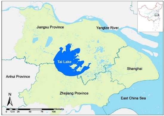
Figure 1.
Location and area of Lake Taihu.
The wind effect is perpetual and can be dominant while the wind has obvious characteristics. It is very important to find out how the wind influences transport and sedimentation. There are several ways to obtain the total suspended particulate matter (TSM) data of a certain water area. Field measurements to obtain sediment data in lakes and reservoirs can be very expensive, time consuming, and are very hard to obtain with full-scale [4]. The remote sensing data is very useful to study in a long time series and over a large area [5,6,7,8]. But it is not always good at obtaining specific time and location because there is no or only partial correct data due to cloud coverage and the temporal resolution is limited by the satellite. Computational fluid dynamics (CFD) is a powerful tool to obtain complete high spatial and temporal resolution data [9,10,11,12,13,14,15,16,17,18,19,20,21,22,23,24,25]. But it needs to be verified to be correct.
In this study, a two-dimensional (2D) model couples the dynamics of shallow water and sediment transport [19]. Suspended sediment transport is simulated with a resuspension and deposition process under wind effect [19]. The 2D model is applied to study the sediment transport and sedimentation in Lake Taihu. Moreover, the TSM is retrieved by the world’s first geostationary satellite ocean color sensor Geostationary Ocean Color Imager (GOCI), using our proposed atmospheric correction algorithm for turbid waters using ultraviolet wavelengths (UV-AC) and regional empirical TSM algorithm [5,7,8]. The model results are validated by GOCI satellite data. The rest of this paper is organized as follows: Section 2 presents the methods of the TSM data obtained from the field measurements, GOCI retrieval, and simulation. In Section 3, the 2D shallow water and sediment transport model is described in detail. The results are presented and discussed in Section 4. Finally, Section 5 draws conclusions for the study.
2. Data and Method
2.1. Data Preparation
TSM data from Lake Taihu are obtained in several ways in this paper. One is from the field measurements on 26 July 2017. Figure 2 shows the research voyage track. The black points in the figure show the exact location of the sampling stations where the TSM is measured. The north point is the 1st station and the cruise went clockwise until the last station, which is the 16th point. TSM was measured gravimetrically on pre-weighed cellulose acetate membrane filters (47 mm diameter, 0.45 µm pore size). Sufficient samples of surface-layer water were collected and filtered at each station to determine the weight of the particulate matter. The filters were frozen and stored below −20 °C until laboratory processing. In the laboratory, the filters were dried in an oven at 40 °C for 6–8 h, then placed in the silica gel drier for 6–8 h, and finally re-weighed to obtain the TSM concentration using the electronic balance. There was at least one blank sample at each station to make the blank correction. The accuracy of the electronic balance is 0.01 mg. In addition, at each station, the remote sensing reflectance () was measured aboard a ship using an ASD FieldSpec®3 full range (350–2500 nm). We measured the upward radiance from the water surface ) and the standard reflecting plate (), and the downward sky radiance (). To avoid sun-glint contamination, the zenith and azimuth angles used to measure were about 40° and 135° (referring to solar orientation), respectively. In addition, we selected an optimal place to minimize the effects of ship shading and foam. Finally, the remote sensing reflectance () was estimated from the measured , and .
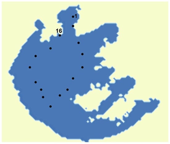
Figure 2.
Locations of the stations where the total suspended particulate matter (TSM) was measured.
The second way TSM data were estimated was by satellite observations using our proposed UV-AC atmospheric correction algorithm and regional empirical TSM algorithm from GOCI. The details are described in Section 2.2. The wind data are implemented in the simulation as a perpetual condition. The wind data is from the European Centre for Medium-Range Weather Forecasts (ECMWF). It has U and a V component of velocity data in the NetCDF format and the temporal resolution is 6 hours.
2.2. Satellite Data Processing
The in-orbit operation of the world’s first geostationary satellite ocean color sensor, GOCI, provides hourly observations. GOCI has eight visible to near-infrared bands (412 nm, 443 nm, 490 nm, 555 nm, 660 nm, 680 nm, 745 nm and 865 nm) with high signal-to-noise ratios, enabling a more accurate retrieval of TSM and other ocean color information [5]. The GOCI observing area is about 2500 km × 2500 km (116.08°E–143.92°E, 24.75°N–47.25°N for central directions) centered on 130°E and 36°N, covering the coasts of Eastern China, the Korean peninsula, and Japan, along with the corresponding shelves and open oceans [6]. Lake Taihu is in the region of the coasts of Eastern China, and the TSM is high in Lake Taihu. To better retrieve the TSM in turbid water, our practical UV-AC atmospheric correction algorithm for GOCI data in turbid waters is used [7].
To overcome the difficulty of the atmospheric correction in turbid waters in Lake Taihu, the UV-AC algorithm was adopted to retrieve the remote sensing reflectance from the GOCI Level-1B data provided by Korean Ocean Research and Development Institute (KORDI). The UV-AC algorithm is based on the fact that in turbid waters, water-leaving radiances increase dramatically at the visible light (VIS) and NIR due to strong particulate scattering caused by high TSM concentrations, but the water-leaving radiance at the ultraviolet band (UV) can be neglected when compared with the VIS and NIR due to the strong absorptions by rich detritus and CDOM. Thus, the UV band can be used to estimate the aerosol scattering reflectance. Since GOCI has no UV band, the shortest blue band (412 nm) was used as the referenced band to retrieve the remote sensing reflectance for the further calculation of TSM. The applicable 412 nm-based UV-AC algorithm to the GOCI data has already been validated in our previous works in the different turbid coastal waters (the Changjiang River Estuary, the Mississippi River Estuary, and the Orinoco River Estuary) [5,7].
2.3. Algorithm Development
For the inland lake, the regional TSM algorithm for GOCI is developed from our previous researches [8]. The reference suggests that it would be better to use the near-infrared wavelength to retrieve the TSM in the Hangzhou Bay (HZB), and develop an empirical TSM model for Medium Resolution Imaging Spectrometer (MERIS) using the ratio of normalized water-leaving radiances between 779 nm and 560 nm. The in situ TSM and at the GOCI bands measured during the summer and winter cruises of the ‘908 Project’ indicate a good correlation between the TSM on the logarithmic scale and the band ratio of at 745 nm and 490 nm from moderately to extremely turbid waters (TSM from 8 mg/l to 5275 mg/l) in the Changjiang River Estuary and HZB [5] as
where and are two coefficients of the empirical TSM algorithm. In the case of HZB [5], they are 1.0758 and 1.1230 for the East China sea respectively. But due to different water quality and TSM sediments, it is found that there is some bias in Lake Taihu. Therefore, the coefficients are recalibrated by linear regression in a semi-logarithmic scale using the TSM algorithm and our field data, based on the experimental results from our research cruise in July 2017.
2.4. Model Simulation
As mentioned above, Lake Taihu has an area of about 2338 km2 and a mean depth of 1.9 m. Due to the aspect ratio of the dimensions of Lake Taihu, a two-dimensional simulation is more than sufficient. Few studies have been conducted that include the sediment deposition and resuspension effects in the finite difference sediment transport model [16,17,18]. Therefore, a 2D numerical model has been developed to simulate the circulation and sediment transport in shallow water systems including the sediment deposition and resuspension effects with proven accuracy when compared to measurements [19].
The shallow water equations are solved by a semi-implicit finite difference method on a non-body-fitted staggered Cartesian grid [10]. The method has been further improved by adapting an Alternating–Direction Implicit method [11]. The convective terms are discretized by an explicit second-order upwind scheme in space [15]. The resultant shallow water model is second-order accurate in both time and space. The standard Eulerian sediment transport equation [16,18,19,20,21] is solved by using a second-order explicit method of central difference in space and two-step Adams–Bashforth in time [19], and the resulting sediment transport model is second-order accurate in both time and space.
To better understand the dynamics of shallow water and sediment transport in practice, the shallow water model [19] is further improved by accounting for wind velocity on the water surface for the effects of wind stress on the flow velocity. Specifically, the wind friction coefficient is determined based on an empirical function using water depth and wind speed, and the atmospheric shear stress at the air-water interface is calculated based on the air density, wind friction coefficient, and wind speed [22,23]. In addition, the current model is further developed to simulate bed topography evolutions based on sediment deposition and resuspension rates [24], which can provide very useful information for sedimentation management and developing dredging strategies in lakes and reservoirs.
3. Implementation of the Numerical Model
3.1. Shallow Water Model
The water depth in surface water systems such as rivers, lakes, and reservoirs is typically much smaller than the horizontal scale, and the flows are characterized by horizontal motions. The hydrostatic assumption is often used to replace the momentum equation in the vertical direction and the vertical acceleration terms are ignored in 2D shallow water equations.
A typical water column is defined in Figure 3, where is the water depth measured from the undisturbed water surface, is the water surface elevation, and is the total depth of the water column, where .
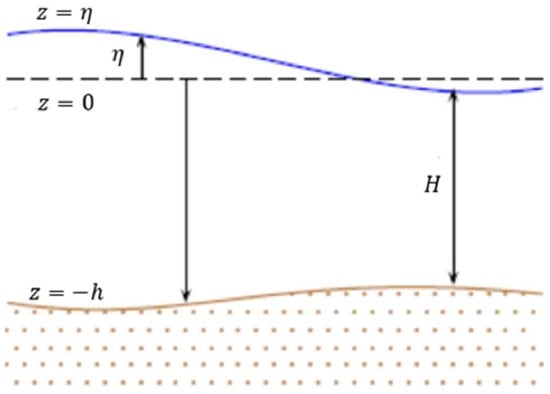
Figure 3.
Geometry of a typical water column.
The model uses a semi-implicit finite difference method on a non-body-fitted staggered Cartesian grid, which has been widely used in shallow water applications with proven accuracy [14,15,19,25]. In this study, the model is further developed by including depth-averaged wind stress terms to account for the effects of wind on the flow velocity. The shallow water equations with wind stress terms have the following form [10],
where and are the depth-averaged velocities components in the x- and y-directions, is the water depth measured from the undisturbed water surface, is the free surface elevation also measured from the undisturbed water surface, is the gravitational acceleration, is the Coriolis frequency, and are the depth-averaged wind stress terms in the and directions, and is the bottom friction coefficient defined as [10],
where is the Chezy friction coefficient, which is defined as [10],
where n is the Manning’s roughness coefficient, is the total water depth defined as
The method to determine the wind shear stress is by this expression [23],
where is the wind shear stress, is the air density, is the wind speed, and is the atmosphere drag coefficient appropriate for wind referenced to a height of 10 m, which is determined based on experiments [22],
The depth-averaged wind shear stress terms can be expressed as [10]
where is the water density, and is the wind direction measured counter-clockwise from the east.
3.2. Sediment Transport Model
The sediment transport model is developed based on the Eulerian transport model including the deposition and resuspension effects. The model has been widely used in sediment transport studies with proven accuracy. The description of the model can be expressed as [16],
where is the depth-averaged suspended sediment concentration, is the diffusion coefficient, is the resuspension rate and is the deposition rate.
The deposition rate is given as [19],
where is the critical deposition shear stress and is the bed shear stress. When is larger or equal to , the deposition rate is zero. When is less than , deposition happens. The settling velocity, , is calculated based on Stokes Law [26] for spherical particles given as,
where is the density of sediment particle, is the density of water, is the diameter of the sediment particle and is the dynamic viscosity of water.
The resuspension rate is calculated as [25],
where is the critical erosion shear stress, is the erosion rate constant and is the erosion exponent. and are case-dependent parameters which can be determined by experiments. When is larger than , resuspension occurs. When is less or equal to , the resuspension rate is zero. When , both the deposition rate and resuspension rate are zero, which means neither deposition nor erosion occurs.
The bed shear stresses are calculated as [27],
where is the flow rate vector, is the norm of , and is the bed friction coefficient defined as
where is the Manning’s roughness coefficient, and is the total depth.
The bed topography evolution is calculated based on the deposition and resuspension rates as [28],
where is the bed displacement and is the dry bulk density. The equation can be solved by the forward Euler method, and the accumulated bed displacement can be determined by summing the bed displacement at each time step.
To solve the sediment transport equation, Equation. (9), a second-order explicit method of central difference in space and two-step Adams–Bashforth in time is used [19], which is not restrictive for simulations in lakes and reservoirs based on previous and current studies.
In summary, Equation (2) solves the general motion of the water using the shallow water model. Equation (10) and Equation (12) solves the deposition rate and the resuspension rate, which are two key variables for the sediment transport model of Equation (9). Once we have the water velocity components, the total water depth is solved from the shallow water model and the deposition or resuspension rate calculated, the sediment transport model of Equation (9) can be solved. On the other hand, Equation (15) solves the bed displacement based on the deposition rate and resuspension rate.
4. Results and Discussions
4.1. GOCI-Retrieved TSM Distributions
Using the method of atmospheric correction algorithm and the regional TSM model following Equation (1), the coefficients and are found by curve fitting cruise measured TSM data on 26 July 2017. Figure 4a shows the resultant linear regression of the empirical TSM algorithm. After recalibration, and are 0.61 and 1.43 respectively. The cruise TSM data measured on Lake Taihu in July 2017 and at the GOCI bands indicate a good correlation between the TSM on the logarithmic scale and the band ratio of at 745 nm over 490 nm with a correlation coefficient of 0.85. Figure 4b shows the comparison of the experiment data and both TSM algorithms before and after the recalibration of the and , with the root mean square errors (RMSE) of 2.83. The black square indicates the experiment data from cruise, the red triangle shows the resultant TSM using the coefficients of reference, and the blue diamond is what we get after the coefficients are changed. It clearly shows the TSM is much larger than the cruise data using the original coefficients.
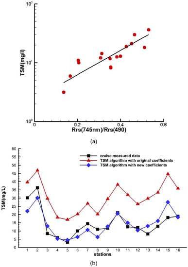
Figure 4.
(a) Linear regression of empirical TSM algorithm and (b) comparison of measured data with TSM algorithm.
Figure 5 shows the resultant monthly average TSM concentration in Lake Taihu retrieved by GOCI in 2017. Each of these outcomes represents the TSM concentration results averaged from days for a certain month. The color bar on the right indicates that the TSM concentration in Lake Taihu ranges from 0 to 400 mg/l approximately. From the monthly TSM concentration results in the contours, the high TSM region is southwest of the lake and is relatively low from January to March. From February to May, the concentration increases and starts to move towards north. And then it decreases and becomes the lowest in July. From July to December, the concentration increases again and keeps filling the entire Lake Taihu from the north lakeshore.
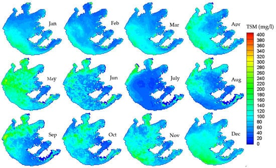
Figure 5.
Monthly average TSM contour of Lake Taihu retrieved by GOCI of year 2017 using calibrated TSM algorithm
4.2. Model-Simulated TSM
The figures above show that remote sensing is very powerful for long time series TSM data. But to study the short duration process of the TSM movement, simulations need to be done when there are obvious characteristics of wind. Figure 6a shows the computational domain of Lake Taihu. It is a rectangular staggered Cartesian grid and the area fits the water area of Lake Taihu. The size of the computational domain is 82 km by 69 km. A grid size of ∆x=∆y=923.5 m is used based on the resolution of GOCI data. The information of sediment particle is collected from experiment [4]. The particle size is 18 and density is 1.5 103 . The main source TSM is from initial input and resuspension. From our experiment in this paper, most of it is inorganic. Figure 6b shows the relative location of the computation domain and wind velocity data from ECMWF. The blue points are the locations of the wind data from ECMWF and the values are projected to the computational grid points using bilinear interpolation.
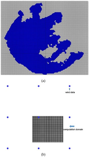
Figure 6.
(a) Computational domain of Lake Taihu and (b) Relative location of the computation domain and wind velocity data from European Centre for Medium-Range Weather Forecasts (ECMWF).
To simulate the sediment transport and sedimentation under wind effect, the time window is considered based on the wind when it has strong characteristics. The case study began March 5 and lasted for 10 days when the wind is mostly east but changes periodically between north and south. Figure 7a shows the average wind history of the entire month of March above the area of Lake Taihu. The red line and blue line represent the U and V component wind velocity respectively. Day 0 means March 5. Figure 7b,c show the resultant water velocity contour and vector after 5 days and 8 days respectively. Due to the complicated topography of eastern Lake Taihu, the water flow circling is mainly determined by the west part of the lake. When the wind is southeast after 5 days from the beginning, the flow moves clockwise and velocity is large relatively. When the wind is northeast after 8 days, the flow change direction is anticlockwise but it is relatively weak. After this 10 day period, the TSM distribution is simulated and Figure 8 shows the results.
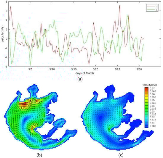
Figure 7.
(a) Average wind velocity components above Lake Taihu in March and (b) water velocity contour and vector after 5 days and (c) 8 days.
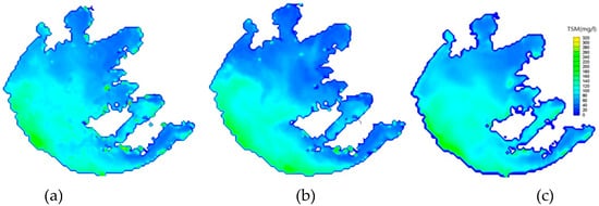
Figure 8.
(a) Initial TSM concentration distribution, (b) TSM concentration distribution after 10 days by GOCI data and (c) simulation results after 10 days.
Figure 8a is the initial TSM concentration distribution at the beginning of the retrieved GOCI simulation. The high TSM concentration area is at the southwest part of the lake and highest close to the lakeshore. Figure 8b represents the distribution after 10 days calculated from the GOCI data, while Figure 8c shows the simulation result after 10 days. Due to the dominant clockwise flow, the TSM concentration results from the simulation under wind effect shows that it is even higher at the lakeshore and the highest TSM region spread to the entire southwest lakeshore. The same results can be found from the GOCI results after 10 days. Both from observation and simulation, the trend of the TSM concentration is to gather along the entire southwest lakeshore. Overall, the spatial distributions of the model simulated TSM are consistent with the GOCI observations.
4.3. Sedimentation in Lake Taihu
Figure 9 shows the bed displacement result from the simulation. In general, the sedimentation is positive in almost all the area of the lake. The greatest deposition is as large as 0.1 meter in this 10 day period simulation. This means the deposition rate is greater than the resuspension rate, which means that most of the time the shear stress created by the wind is less than both the critical resuspension shear stress and the critical deposition shear stress. The location of where the large amount of the deposition happens can be explained by incorporating the velocity and TSM concentration results in Figure 7 and Figure 8. There are two different situations where sedimentation occurs. One is where the velocity is always low and the TSM concentration is not the highest, giving a large deposition rate, such as the zigzag lakeshore at the east and north of the lake, as well as the area around the mid-lake island. The other one is that the concentration is the highest and velocity is large most of the time, such as at the southeast lakeshore. This agrees with the equation from Equation (10) to Equation (15). Either the large concentration or the deposition duration will result in a relatively big deposition in total, so long as it fits the deposition condition.
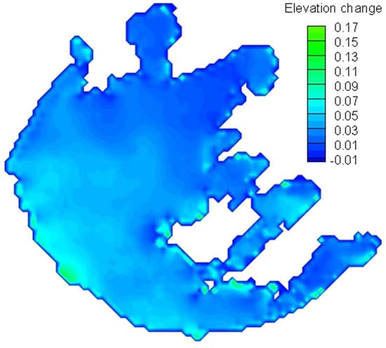
Figure 9.
Change of bed elevation.
5. Conclusion
Remote sensing data from GOCI has been processed using the UV-AC atmospheric correction algorithm and the empirical TSM model to obtain the monthly averaged TSM distribution in Lake Taihu. It indicates that the TSM concentration in Lake Taihu ranges from 0 to 400 mg/l. The high TSM concentration region is clearly shown in each month. The empirical TSM algorithm for Lake Taihu was established by recalibrating the coefficients of our previous algorithm developed for Hangzhou Bay. After recalibration, α and β are 0.61 and 1.43 respectively for Equation (1). Moreover, a hydrodynamic and sedimentation simulation has been completed, which uses wind conditions provided by ECMWF and the GOCI-retrieved TSM data. A case starting March 5 and running for 10 days is presented in this study. The simulation shows good agreement of the TSM between GOCI observation data and simulation results. The trend of the TSM concentration is to gather to the entire southwest lakeshore, both from observation and simulation. In addition, the final sedimentation results show a very rationale topology, which is matched by the theoretical equation with velocity and TSM results. The sedimentation happens mostly where the velocity is always low, such as at the zigzag lakeshore at the east and north of the lake, as well as the area around the mid-lake island and where the concentration is the highest, such as at the southeast lakeshore. This indicates that either the large concentration or the deposition duration will result in a relatively big deposition in total, as long as it fits the deposition condition. It reveals the dangerous locations that need to be observed and desilted.
We have succeeded in estimating the sedimentation on the bottom bed of Lake Taihu using a numerical simulation combined with geostationary satellite ocean color data. However, there is still some room for improvement in our work. The parameters in our TSM algorithm are based on the experimental results from a research cruise in July 2017. Limited by the in-situ data, we cannot obtain experiment data covering different seasons. However, changes to the parameters for different seasons will obtain more accurate TSM retrieval. Therefore, we are planning to do another field measurement in a different season and at locations where the TSM is potentially high. On the other hand, river input and output are neglected as the wind driven current is dominant for the change of TSM in this 10-day short term simulation. As a fact, adding river data into the simulation is our near-term target and we believe it will be more realistic and beneficial for a long term simulation.
Author Contributions
Conceptualization, A.H. Methodology, A.H., X.H. and Y.B. Software, A.H. and X.H. Validation, A.H. Resources, F.G. and Q.Z. Data curation, F.G. and Q.Z. Writing—original draft preparation, A.H. Writing—review and editing, X.H. and D.P. Supervision, H.H. Project administration, X.H. Funding acquisition, X.H.
Funding
This research was supported by the National Key Research and Development Program of China (Grant #2017YFA0603003), the National Basic Research Program (973 Program) of China (Grant #2015CB954002), the Public Science and Technology Research Funds Projects for Ocean Research (Grant #201505003), the National Natural Science Foundation of China (Grants #41676172, #41676170, #41825014 and #41621064), and the Project of State Key Laboratory of Satellite Ocean Environment Dynamics (Grant #SOEDZZ1801).
Acknowledgments
We thank the satellite ground station and the satellite data processing and sharing center of SOED/SIO for help with the data processing. All authors would like to thank the reviewers for their detailed and critical comments and helpful suggestions.
Conflicts of Interest
The authors declare no conflict of interest.
References
- Zhang, F.; Lee, J.; Liang, S.; Shum, C.K. Cyanobacteria blooms and non-alcoholic liver disease: Evidence from a county level ecological study in the United States. Environ. Health 2015, 14, 41. [Google Scholar] [CrossRef] [PubMed]
- Liu, B.; Wei, Q.; Zhang, B.; Bi, J. Life cycle GHG emissions of sewage sludge treatment and disposal options in Tai lake. Sci. Total Environ. 2013, 447, 361–369. [Google Scholar] [CrossRef] [PubMed]
- Qin, B.; Xu, P.; Wu, Q.; Luo, C.; Zhang, Y. Environmental issues of lake Taihu. China Hydrobiol. 2007, 581, 3–14. [Google Scholar] [CrossRef]
- Qin, B.; Hu, W.; Gao, G.; Luo, L.; Zhang, J. Dynamics of sediment resuspension and the conceptual schema of nutrient release in the large shallow Lake Taihu, China. Chin. Sci. Bull. 2004, 49, 54–64. [Google Scholar] [CrossRef]
- He, X.; Bai, Y.; Pan, D.; Huang, N.; Dong, X.; Chen, J.; Chen, C.; Cui, Q. Using geostationary satellite ocean color data to map the diurnal dynamics of suspended particulate matter in coastal waters. Remote Sens. Environ. 2013, 133, 225–239. [Google Scholar] [CrossRef]
- Ryu, J.H.; Choi, J.K.; Eom, J.; Ahn, J.H. Temporal variation in Korean coastal waters using Geostationary Ocean Color Imager. J. Coast. Res. 2011, SI64, 1731–1735. [Google Scholar]
- He, X.; Bai, Y.; Pan, D.; Tang, J.; Wang, D. Atmospheric correction of satellite ocean color imagery using the ultraviolet wavelength for highly turbid waters. Opt. Express 2012, 20, 20754–20770. [Google Scholar] [CrossRef] [PubMed]
- Bai, Y.; He, X.Q.; Pan, D.L.; Zhu, Q.K.; Lei, H.; Tao, B.Y.; Hao, Z. The extremely high concentration of suspended particulate matter in Changjiang Estuary detected by MERIS data. Proc. SPIE 2011, 7858, 78581D. [Google Scholar]
- Spaulding, M.L. Laterally integrated numerical water quality model for an estuary. J. Fluids Eng. 1974, 96, 103–110. [Google Scholar] [CrossRef]
- Casulli, V. Semi-implicit finite difference methods for the two-dimensional shallow water equations. J. Comput. Phys. 1990, 86, 56–74. [Google Scholar] [CrossRef]
- Spall, R.E.; Addley, C.; Hardy, T. Numerical analysis of large gravel-bed rivers using the depth averaged equations of motion. In Proceedings of the ASME FEDSM01, FEDSM2001-18169, New Orleans, LA, USA, 29 May–1 June 2001. [Google Scholar]
- Zheng, Z.C.; Zhang, N. A hydrodynamic simulation for Mobile Bay circulation. In ASME 2002 International Mechanical Engineering Congress and Exposition; American Society of Mechanical Engineers: New Orleans, LA, USA; 17–22 November 2002, pp. 735–740.
- Langevin, C.; Swain, E.; Wolfert, M. Simulation of integrated surface-water/ground-water flow and salinity for a coastal wetland and adjacent estuary. J. Hydrol. 2005, 314, 212–234. [Google Scholar] [CrossRef]
- Zhang, N.; Yadagiri, S. Numerical Investigation of the Impact of Calcasieu Ship Channel on the Hydrodynamics and Water-Substance Transport in Calcasieu Lake and Surrounding Wetlands. In ASME 2010 3rd Joint US-European Fluids Engineering Summer Meeting Collocated with 8th International Conference on Nanochannels, Microchannels, and Minichannels; American Society of Mechanical Engineers: Montreal, QC, Canada; 1–5 August 2010, pp. 181–186.
- Zhang, N.; Zheng, Z.C.; Yadagiri, S. A hydrodynamic simulation for the circulation and transport in coastal watersheds. Comput. Fluids 2011, 47, 178–188. [Google Scholar] [CrossRef]
- Shrestha, P.L. An integrated model suite for sediment and pollutant transport in shallow lakes. Adv. Eng. Softw. 1996, 27, 201–212. [Google Scholar] [CrossRef]
- Shrestha, P.L.; Blumberg, A.F.; DiToro, D.M.; Hellweger, F. A Three-Dimensional Model for Cohesive Sediment Dynamics in Shallow Bays. In Proceedings of the 2000 Joint Conference on Water Resources Engineering and Water Resources Planning and Management, Minneapolis, Minnesota, 30 July–2 August 2000; pp. 1–10. [Google Scholar]
- Umita, T.; Kusuda, T.; Futawatari, T.; Awaya, Y. Study on erosional process of soft mud. Jpn. Soc. Civ. Eng. 1988, 393, 33–42. [Google Scholar]
- Zhang, N.; Kee, D.; Li, P. Investigation of the impacts of Gulf sediments on Calcasieu Ship Channel and surrounding water systems. Comput. Fluids 2013, 77, 125–133. [Google Scholar] [CrossRef]
- Kondo, M. Physical properties of cohesive sediment materials and characteristics of their erosion by flow. Trans. JSIDRE 1993, 163, 79–86. [Google Scholar]
- Hiramatsu, K.; Shikasho, S.; Mori, K. Numerical prediction of suspended sediment concentrations in the Ariake Sea, Japan, using a time-dependent sediment resuspension and deposition model. Paddy Water Environ. 2005, 3, 13–19. [Google Scholar] [CrossRef]
- Teeter, A.M. Sediment Resuspension and Circulation of Dredged Material in Laguna Madre, Texas; Technical Report; US Army Engineer Research and Development Center: Vicksburg, MS, USA, 2001. [Google Scholar]
- Teeter, A.M.; Johnson, B.H.; Berger, C.; Stelling, G.; Scheffner, N.W.; Garcia, M.H.; Parchure, T.M. Hydrodynamic and sediment transport modeling with emphasis on shallow-water, vegetated areas (lakes, reservoirs, estuaries and lagoons). Hydrobiologia 2001, 444, 1–23. [Google Scholar] [CrossRef]
- Lee, C.; Schwab, D.J.; Beletsky, D.; Stroud, J.; Lesht, B. Numerical modeling of mixed sediment resuspension, transport, and deposition during the March 1998 episodic events in southern Lake Michigan. J. Geophys. Res. Oceans 2007. [Google Scholar] [CrossRef]
- Zhang, N.; Li, P.; He, A. Coupling of One-Dimensional and Two-Dimensional Hydrodynamic Models Using an Immersed-Boundary Method. J. Fluids Eng. 2014, 136, 040907. [Google Scholar] [CrossRef]
- Lamb, H. Hydrodynamics; Cambridge University Press: Cambridge, UK, 1932. [Google Scholar]
- Vreugdenhil, C.B. Numerical Methods for Shallow-Water Flow; Springer Science & Business Media: Berlin, Germany, 2013; Volume 13. [Google Scholar]
- Berger, R.C.; Tate, J.N.; Brown, G.L.; Savant, G. Guidelines for Solving Two-Dimensional Shallow Water Problems with the Adaptive Hydraulics (ADH) Modeling System; USACE Research and Development Center: Vicksburg, MS, USA, 2008. [Google Scholar]
© 2019 by the authors. Licensee MDPI, Basel, Switzerland. This article is an open access article distributed under the terms and conditions of the Creative Commons Attribution (CC BY) license (http://creativecommons.org/licenses/by/4.0/).