Building A High-Resolution Vegetation Outlook Model to Monitor Agricultural Drought for the Upper Blue Nile Basin, Ethiopia

Abstract

To reduce the impacts of drought, developing an integrated drought monitoring tool and early warning system is crucial and more effective than the crisis management approach that is commonly used in developing countries like Ethiopia. The overarching goal of this study was to develop a higher-spatial-resolution vegetation outlook (VegOut-UBN) model that integrates multiple satellite, climatic, and biophysical input variables for the Upper Blue Nile (UBN) basin. VegOut-UBN uses current and historical observations in predicting the vegetation condition at multiple leading time steps of 1, 3, 6, and 9 dekades. VegOut-UBN was developed to predict the vegetation condition during the main crop-growing season locally called “Kiremt” (June to September) using historical input data from 2001 to 2016. The rule-based regression tree approach was used to develop the relationship between the predictand and predictor variables. The results for the recent historic drought (2009 and 2015) and non-drought (2007) years are presented to evaluate the model accuracy during extreme weather conditions. The result, in general, shows that the predictive accuracy of the model decreases as the prediction interval increases for the cross-validation years. The coefficient of determination (R²) of the predictive and observed vegetation condition shows a higher value (R² > 0.8) for one-month prediction and a relatively lower value (R² ≅ 0.70) for three-month prediction. The result also reveals strong spatial integrity and similarity of the observed and predicted maps. VegOut-UBN was evaluated and compared with the Standardized Precipitation Index (SPI) (derived from independent rainfall datasets from meteorological stations) at different aggregate periods and with a food security status map. The result was encouraging and indicative of the potential application of VegOut-UBN for drought monitoring and prediction. The VegOut-UBN model could be informative in decision-making processes and could contribute to the development of operational drought monitoring and predictive models for the UBN basin.

1. Introduction

A vegetation-condition-based drought monitoring and prediction model is vital to enhance knowledge-based decision-making processes in areas where economic growth is dependent on rain-fed agriculture. Agriculture, the most drought-vulnerable sector, needs a proactive risk management approach to mitigate the adverse impacts associated with the occurrence of drought. In Ethiopia, agriculture is the main income-generating sector, accounting for over half of the total Gross Domestic Product (GDP) of the country [1,2]. Failure of the annual rainfall is closely associated with failure of the crop production, which eventually affects the socio-economic sector of the country. The drought that occurred in 2015 affected the annual crop yield and production, which exacerbated food insecurity in most of the farming regions in the country [3]. According to the UN Office for the Coordination of Humanitarian Affairs (OCHA), more than 4 million people have needed food aid and humanitarian assistance in Ethiopia since the beginning of 2015 [4]. Hence, crop yield reduction is closely associated with the failure of the annual rainfall and poor vegetation condition. Other notable historic drought events (e.g., 1983–1984, 1994–1995, 2003–2004, and 2009–2010) have occurred in the country and caused devastation in terms of the loss of human lives and reduction in annual crop production [5,6]. This indicates the existence of a strong linkage between crop production and drought in Ethiopia. Developing a vegetation condition prediction model greatly enhances the potential to estimate the annual crop yield production that, in turn, supports developing food security and drought early warning systems [7,8,9].

Monitoring vegetation condition, referred to in this study as “vegetation greenness”, involves the use of mainly the remote-sensing-based Normalized Difference Vegetation Index (NDVI), which is computed using the spectral reflectance acquired in the near-infrared (NIR) and red band regions [10]. NDVI reflects the greenness of the vegetation and/or the vegetation health. Low NDVI values indicate drought conditions whereas high NDVI values show healthy vegetation conditions [11]. The response of the vegetation condition reflects the cumulative effects of climatic, oceanic, topographic, and other biophysical variables, indicating the complexity and integral challenges in predicting the vegetation condition. Nevertheless, an integral approach enhances understanding of the complex natural phenomena and interconnections among the different components of the hydrologic cycle. The availability of good-quality long-term remote sensing and ground-based observations in environmental datasets allows for the development of advanced data mining and other techniques that could help in extracting useful information in support of informative decision-making processes [12,13]. Many previous studies indicated strong teleconnections between drought occurrence and El Niño southern oscillation (ENSO), sea surface temperature (SST) anomalies in the southern Atlantic and Indian oceans, and other anthropogenic activities that exacerbate land use change in Ethiopia [14]. Thus, an integral approach that includes the potential use of oceanic indices contributes to the development of a robust drought prediction model for Ethiopia.

The advancement of remote sensing technology enhanced the capability of prediction of vegetation condition, particularly in data-scarce regions [15]. The availability of spatially continuous and high-temporal-resolution measurements from remote sensing products leverages an increasing demand for knowledge-based decision-making processes for drought planning [16,17]. Extracting valuable information from the data helps to support strong decision-making processes. Data mining techniques play a great role in terms of handling Big Data and identifying the pattern and relationships among the input parameters, and they generate new knowledge about the dataset [18]. There are several predictive and descriptive data mining techniques. The regression tree data mining technique is the most commonly and widely used approach in drought studies [19,20]. The decision trees are represented in the form of a tree structure with different nodes. Even though drought is a complex atmospheric phenomenon, the data mining technique is able to capture its spatial and temporal patterns through knowledge developed from the huge dataset.

Many studies have noted the potential usefulness of VegOut in drought monitoring and preparedness activities across the world. Most of the studies supported the integral approach of using several environmental datasets to monitor and predict vegetation conditions in different agro-climatic zones. For example, Tadesse et al. [20] developed a VegOut model for Nebraska and South Dakota in the USA, and they reported the applicability of VegOut in predicting the vegetation condition to a certain leading time. A similar approach was presented by expanding the study area over the central United States to support the usefulness of VegOut for drought monitoring by Tadesse et al. [21]. Tadesse et al. [22] studied the predictive capability of VegOut to monitor vegetation stress during the crop-growing season in Ethiopia. The model performed well in indicating vegetation stress across the drought-prone parts of the country when evaluated for the selected historic drought years. Several other studies also indicated a strong link between vegetation vigor and oceanic indices [23], soil moisture condition [10], and other parameters [24]. Most VegOut-related studies are of a large scale—for example, continental [13,25] and country level [22]. However, only very limited efforts have been made to develop and test VegOut at relatively finer spatial resolutions (250 m × 250 m) and at a catchment and basin level in rugged topography where the orographic effects of rainfall and local climatic conditions significantly affect the climate condition [26]. The development of the VegOut model in the Ethiopian highlands is crucial for water resource management. Most of the transboundary rivers originating from the highlands require integrated water resource management to maximize benefits and equitable share of water among the riparian countries.

In this paper, the vegetation outlook (VegOut-UBN) model was developed using several sets of climatic, oceanic, and biophysical data at a finer spatial resolution (250 m × 250 m) for the Upper Blue Nile Basin in Ethiopia. The rule-based regression tree approach was followed to model the relationship that exists between the input variables. This study contributes to developing a knowledge-based approach that could assist decision-makers in mitigating drought and its resulting impacts.

2. Materials and Methods

2.1. Study Area

The UBN Basin is located at the geographic coordinates of 7°40′ and 12°51′N latitudes and 34°06′ and 40°00′E longitudes in the northwestern part of Ethiopia (Figure 1). The basin covers a total area of ~200,000 km² upstream from the Ethiopia–Sudan border [27]. Its altitude ranges from ~490 m in the lowlands at the Ethiopia–Sudan border to ~4260 m in the highlands of Mount Guna. The annual rainfall ranges from 780 mm to 2200 mm, with the highlands having the highest rainfall (ranging from 1500 to 2200 mm) and the lowlands receiving less than 1500 mm [27,28,29]. The main rainfall season (locally called “Kiremt”) in the basin spans from June to September, and 82% of the annual flow occurs during this season [30]. More than 85% of the annual crop is produced during the Kiremt season [31]. The mean annual temperature ranges from 13 °C in southeastern parts to 26 °C in the southwestern part near the Ethiopia–Sudan border [32].

The land cover in the basin is dominated by dry-land, cropland, pastures, savannah, grassland, woodland, water bodies, and sparsely vegetated plants. Cropland is the dominant land use and land cover type, covering 44% of the total area of the basin [33]. Rain-fed agriculture is the dominant practice in the basin, and a variety of crops are grown under rain-fed condition. A large area of bamboo is available in the lowland toward the western part of the basin. Open to dense woodland is abundant in the south, southwest, and southeast parts of the basin, and open shrubland is dominant in the highlands of the basin. Volcanic rock and Precambrian basement rock are the most widely available geological formations in the basin, and small areas are covered by sedimentary rock [27]. The dominant soil types are Leptosols and Alisols (21%), Nitosols (16%), Vertisols (15%), and Cambisols (9%) [34].

2.2. Data Used

Several environmental datasets containing climate, satellite, oceanic, and other static biophysical parameters were used in developing the VegOut-UBN model for the basin. The summaries of the input variables are described in the subsections below and in

Table 1. Summary of the attributes used to develop the VegOut-UBN model.

No.	Attributes	Resolutions		Source
		Spatial	Temporal
1	NDVI-based standardized seasonal greenness (SSG)	250 m	dekadal	eMODIS
2	CHIRPS rainfall	5 km	dekadal	CHG
3	Atlantic Meridional Mode (AMM)	-	monthly	CPC/NOAA
4	Multivariate ENSO index (MEI)	-	monthly	CPC/NOAA
5	Oceanic Niño Index (ONI)	-	monthly	CPC/NOAA
6	Pacific Decadal Oscillation (PDO)	-	monthly	CPC/NOAA
7	Tropical Northern Atlantic Index (TNA)	-	monthly	CPC/NOAA
8	Trans- Niño Index (TNI)	-	monthly	CPC/NOAA
9	Dipole Mode Index (DMI)	-	monthly	CPC/NOAA
10	Digital Elevation Model (DEM)	90 m	-	SRTM
11	Land use/Land cover (LULC)	300 m	-	ESA
12	Available Water Holding Capacity (AWC)	1 km	-	ISRIC-WISE
13	Ecosystem type (eco)	1 km	-	Ecodiv.org
14	Soil moisture	10 km	monthly	FEWS NET

. The data have different spatial resolutions and were resampled to 250 m spatial resolution using the Inverse Distance Weighted (IDW) technique. Because of its consideration of the inverse proportionality with distance, the IDW gives a better representation of a variable over heterogeneous topographic terrain, and it is a widely used technique [6].

2.2.1. Climate Data

Satellite-based Climate Hazards Group InfraRed Precipitation with Station (CHIRPS) data were used in this study [9]. The time series of the data (1981–2016) was downloaded from the Climate Hazards Group (CHG) (http://chg.geog.ucsb.edu/data/chirps/) at a spatial resolution of 5 km × 5 km. The main reason for the use of CHIRPS in this study is because of its accuracy and applications for meteorological drought study in the UBN basin [15]. A recent comparative study of five satellite-based rainfall products supported the best performance of CHIRPS rainfall for the UBN basin [15]. Moreover, a CHIRPS-based Z-score was applied to assess spatiotemporal patterns of meteorological drought in the basin [15]. The Z-score calculation involves an approach similar to that for the common and widely used Standardized Precipitation Index (SPI) [35], except for its assumption of normal distribution of rainfall. Bayissa et al. [6] investigated the best-fitting probability density function (PDF) for the basin using weather-station-based rainfall data. They reported that a normal distribution fits the rainfall in some of the weather stations even though Gamma and other PDFs dominated in the other stations. In this study, the Z-score represents the climatic component in developing the VegOut-UBN model. Besides CHIRPS, the rainfall data for the selected 14 weather stations (Figure 1) were collected from the National Meteorological Agency (NMA) of Ethiopia for 1981–2016.

2.2.2. Satellite Data

MODIS-based dekadal NDVI (eMODIS) data of relatively higher spatial resolutions (250 m × 250 m) were used in this study for the period 2001–2016. These eMODIS time-series data were obtained from the U.S. Geological Survey (USGS) Earth Resources Observation and Science (EROS) Center. The satellite component of the VegOut-UBN model was represented by NDVI-based standardized seasonal greenness (SSG), which provides useful information about the vegetation condition. SSG (Equation (2)) was calculated using Seasonal Greenness (SG), which represents the accumulated NDVI within the starting and ending dekades of the growing season (Equation (1))

$$\mathrm{SG}={{\displaystyle \sum }}_{\mathrm{P}1}^{\mathrm{P}n}({\mathrm{NDVI}}_{\mathrm{p}}-{\mathrm{NDVI}}_{\mathrm{b}})$$

(1)

In Equation (1),

• SG is the seasonal greenness,
• P₁, P₂, …, Pn are dekades within the growing season,
• NDVI_p is the observed dekadal value, and
• NDVI_b is the baseline NDVI value at the beginning of the growing season.

$${\mathrm{SSG}}_i=\frac{{\mathrm{SG}}_i-{\overline{\mathrm{SG}}}_i}{{\mathsf{\sigma }}_i}$$

(2)

In Equation (2),

• ${\mathrm{SSG}}_i$ is the standardized seasonal greenness for each dekade within the growing season or Z-score of seasonal greenness (SG),
• ${\mathrm{SG}}_i$ is the current SG,
• ${\overline{\mathrm{SG}}}_i$ is the average SG observed in the historic record up to time period i, and
• ${\mathsf{\sigma }}_i$ is the standard deviation of the historical ${\mathrm{SG}}_i$ values.

The SSG values range from −4.0 to +4.0, which represent stressed to healthy vegetation conditions, respectively. This range was determined based on the values of the SSG in this study. Since SSG is standardized, it is comparable in both space and time.

2.2.3. Oceanic Indices

Several studies have indicated the strong teleconnection between oceanic indices and the climate in Ethiopia [36,37,38]. A recent study by Degefu et al. [39] supported the strong association of the sea surface temperature (SST) and rainfall in Ethiopia. Thus, integrating oceanic indices into the VegOut-UBN model improves the accuracy of the model’s predictive capability for vegetation condition and drought. Seven oceanic indices—Atlantic Meridional Mode (AMM), Multivariate ENSO index (MEI), Oceanic Niño Index (ONI), Pacific Decadal Oscillation (PDO), Tropical Northern Atlantic Index (TNA), Trans-Niño Index (TNI), and Dipole Mode Index (DMI)—were considered in this study. The time series of the oceanic indices (2001–2016) were obtained from the National Oceanic and Atmospheric Administration (NOAA) Earth System Research Laboratory [40].

2.2.4. Environmental Data

The other environmental datasets considered in this study were the Digital Elevation Model (DEM), Land Use/Land Cover (LULC) type, Available Water Holding Capacity (AWC), and ecosystem type (eco). DEM accounts for the effects of altitude on vegetation condition; the data were obtained from the Shuttle Radar Topography Mission (SRTM) at 90 m × 90 m spatial resolutions. LULC is the other biophysical parameter considered in this study. LULC accounts for the different land cover/land use types in response to the vegetation condition. The LULC map was obtained from the European Space Agency (ESA) at 300 m × 300 m spatial resolution. The water holding capacity (AWC) of the soil represents the amount of water a given soil can hold for plant use. AWC data was obtained from the International Soil Reference and Information Centre - World Inventory of Soil Emission (ISRIC-WISE) reanalyzed soil database [41].

2.2.5. Soil Moisture

Soil moisture data based on the monthly Noah land surface model were obtained from the Famine Early Warning Systems Network (FEWS NET) Land Data Assimilation System (FLDAS) for 2001–2016. Simulation run “C” forced by a combination of Modern Era Retrospective analysis for Research and Applications Version 2 (MERRA-2) and Climate Hazards Group InfraRed Precipitation with Stations (CHIRPS) data was used in this study. The spatial resolution of the soil moisture data was ~10 km and the data were available for different layers of the soil. The average soil moisture at the depth of 40 cm was considered to represent the readily available water at the root depth. Further information about Noah soil moisture can be found in Xia et al. [42].

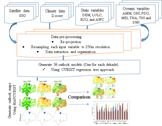
2.3. VegOut-UBN Model Development

Figure 2 summarizes the method followed in this research. Developing a VegOut-UBN model involves the use of several dynamic and static input variables. The dynamic variables vary in space and time while static variables are assumed to be constant for each dekade across the study period. Both sets of the input data were extracted first at the corresponding locations of about 40,000 artificially generated points covering the UBN basin. Each point was located at the center of a ~5 km × ~5 km grid and resulted in 23,040,000 sample values for each input dataset to train in Cubist. We used a one-year data holding approach (“jackknife” test) to train (model construction) and to test the models for each year within the historical records. For example, the 2001 dataset was taken out from the historical records and used to test the model while the remaining datasets (2002–2016) were used to construct (train) the models. This process of the data holding approach was repeated for each year iteratively to evaluate the models.

In this study, the static input variables were assumed to be constant across the study period, and those input variables with monthly temporal scales were assumed to be constant for each dekade of that specific month. Cubist is data mining software [43,44] used to develop the rule-based linear regression trees that represent linear expression to compute the target variable (SSG). SSG is assumed to be a dependent variable that has to be predicted using other input datasets. Equation (3) shows the general form of the rule-based linear regression model defined by Cubist that is used to explain the predictand variable (SSG) using a set of other predictor variables:

VegOut−UBN(i) = ƒ_1,i (SSG)_t=0 + ƒ_2,i(Z-score, SM)_t=0 + ƒ_3,i(DEM, LULC, eco, AWC)_t=0 + ƒ_4,i(AMM, MEI, ONI, PDO, TNA, TNI, DMI)_t=0,

(3)

where VegOut-UBN(i) is the predicted SSG at different dekadal leading time i as a function of the current (t = 0) values of the input variables. The equation shows that the predicted SSG is a function of the current SSG and other dynamic and static variables.

Thus, 36 rule-based models, one for each dekade in a year, were developed and used to predict the target variable (SSG). The rule developed for each dekade comprises several multivariate linear regression equations in the form of “if conditions” as shown below. This example rule shows the “if condition” and the multivariate regression equation used to quantify VegOut-UBN. If the threshold criteria for the set of variables in the “if conditions” are satisfied, then the regression equation is used to determine VegOut-UBN values for all the pixels under similar conditions. The SSG value of the previous dekade was used as an initial condition of the current prediction of the vegetation condition.

Rule 1 (Example):

  if

  DEM > 1558

  AMM > −4.13

  DMI > −3.85

  SM ≤ 3.39

  SSG > −0.13

  then

VegOut-UBN = 43.709 + 0.74 SSG − 0.064 AMM − 0.0025 DMI − 0.19 PNA + 0.09 Z-score − 0.08 SM − 0.007 DEM

2.4. VegOut-UBN Map Generation

The VegOut-UBN map was generated for each dekade within the growing season (June to September). The first dekade of June was selected as a current vegetation condition to predict the vegetation condition for every future dekade within the growing season. However, VegOut-UBN maps generated for leading times of 1 (2nd dekade of June), 3 (1st dekade of July), 6 (1st dekade of August), and 9 dekades (1st dekade of September) are presented to illustrate the VegOut-UBN model result. These leading dekades represent the different stages of plant growth (from germination to maturity) in the UBN basin. VegOut-UBN maps were generated at a spatial resolution of 250 m using the MapCubist software developed at the USGS Center for Earth Resources Observation and Science (EROS). MapCubist used the regression tree rules and the current gridded images of the input data to produce VegOut-UBN for several dekades of certain leading times. For example, the VegOut-UBN map for the 2nd dekade of June (one dekade leading time) was generated using all the gridded input data of the current dekade (1st dekade of June) and regression tree rules developed for the 1st dekade. In this study, the SPI drought categories (

Table 2. Drought categories of the VegOut-UBN model based on Standardized Precipitation Index (SPI) drought categories (McKee et al. [45]).

VegOut-UBN Values	Drought Category
−2.00 and less	Extreme Stress
−1.50 to −1.99	Severe Stress
−1.00 to −1.49	Moderate Stress
−0.5 to −0.99	Poor Vegetation
−0.5 to 0.5	Near Normal
0.5 to 0.99	Fair Vegetation
1.0 to 1.49	Good Vegetation
1.5 to 1.99	Very Good Vegetation
>2.0	Excellent Vegetation

) were adapted to classify the drought categories of VegOut-UBN maps.

2.5. Comparison of VegOut-UBN Model with SPI and Food Security Maps

The VegOut-UBN model was compared with independently measured rainfall data for selected meteorological stations, as shown in Figure 1. The SPI values at 1-, 3-, 6-, 9-, 12-, 24-, and 60-month aggregate periods were calculated for those stations using 20+ years of rainfall data. The values of VegOut-UBN maps at the locations corresponding to the meteorological stations were extracted and compared with the SPI for different aggregate periods. The correlation coefficient statistical technique was used to compare VegOut-UBN with the corresponding SPI values for different aggregate periods. In addition to SPI (2001–2015), the food security status maps of 2009 and 2015 were compared with the average VegOut-UBN of a similar period. The visual comparison was adapted to analyze the similarities and differences between VegOut-UBN and food security maps for 2009 and 2015. The food security maps were obtained from Famine Early Warning Systems (FEWS) and provide objective, evidence-based analysis in an informative decision-making process responding to humanitarian crises. The classification of the food security is based on a convergence of the available data and evidence, including indicators related to food consumption, livelihoods, malnutrition, and mortality. The thresholds of the different classification phases of the food status illustrated based on the Integrated Phase Classification (IPC) are shown in

Table 3. Integrated Phase Classification (IPC) acute food insecurity phase classification. The colors in the first column show the different food security status and having the same meaning as the legend color in Figure 8b,d.

PHASE 1 Minimal	More than four in five households (HHs) are able to meet essential food and nonfood needs without engaging in atypical, unsustainable strategies to access food and income.
PHASE 2 Stressed	Even with any humanitarian assistance at least one in five HHs in the area have the following or worse: minimally adequate food consumption but are unable to afford some essential nonfood expenditures without engaging in irreversible coping strategies.
PHASE 3 Crises	Even with any humanitarian assistance at least one in five HHs in the area have the following or worse: Food consumption gaps with high or above usual acute malnutrition OR Are marginally able to meet minimum food needs only with accelerated depletion of livelihood assets that will lead to food consumption gaps.
PHASE 4 Emergency	Even with any humanitarian assistance at least one in five HHs in the area have the following or worse: Large food consumption gaps resulting in very high acute malnutrition and excess mortality OR Extreme loss of livelihood assets that will lead to food consumption gaps in the short term.
PHASE 5 Famine	Even with any humanitarian assistance at least one in five HHs in the area have an extreme lack of food and other basic needs where starvation, death, and destitution are evident. Evidence for all three criteria (food consumption, acute malnutrition, and mortality) is required to classify Famine.

(Source: IPC 2.0 Technical manual).

. In comparing the VegOut-UBN model with the food security map, there is an assumption of a direct relationship between food insecurity and drought occurrence.

The crop yield data were not used to evaluate the VegOut-UBN model in this study because of its poor quality and coarser spatial resolution as reported in our previous studies [46,47].

3. Results and Discussions

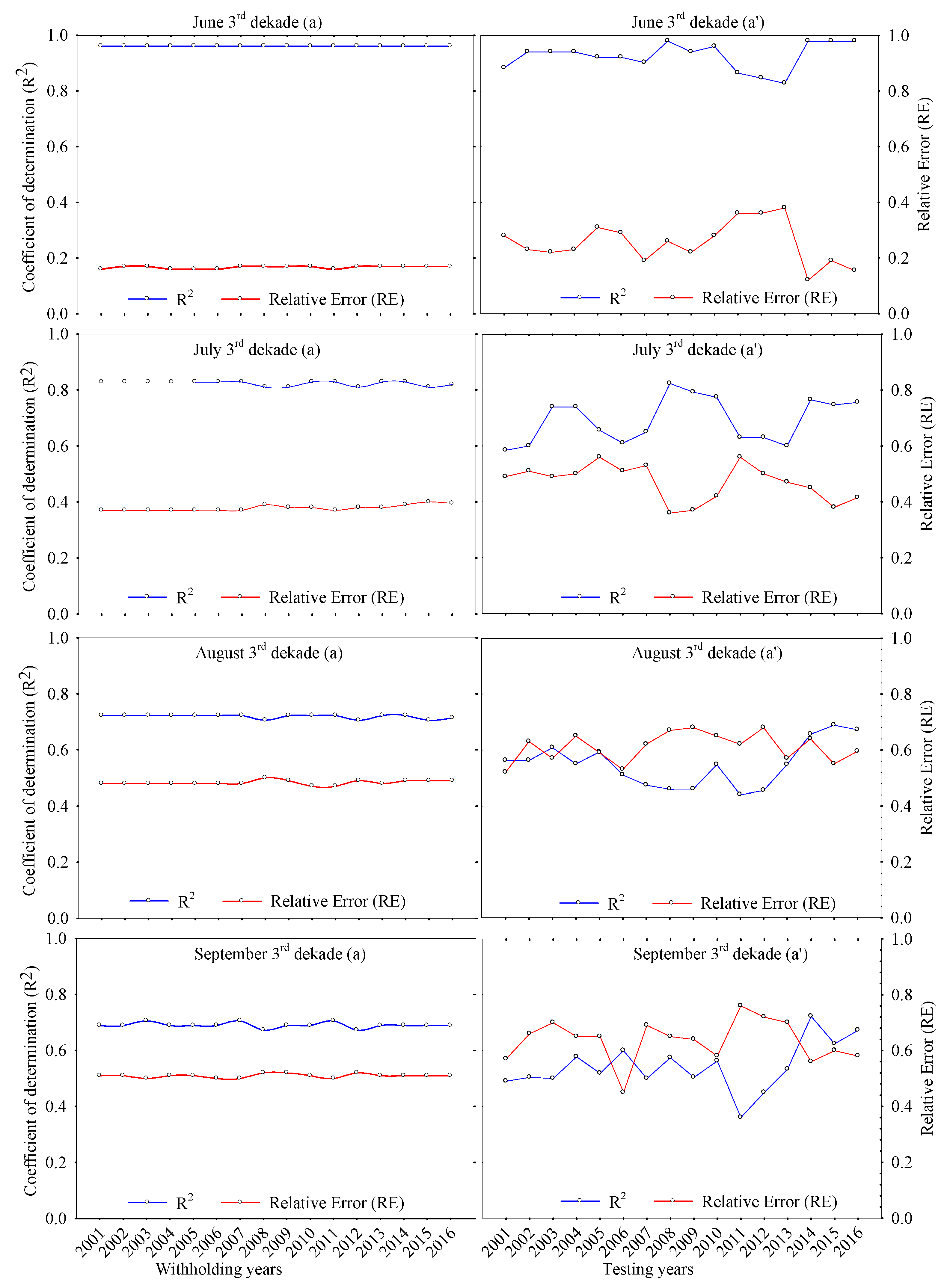
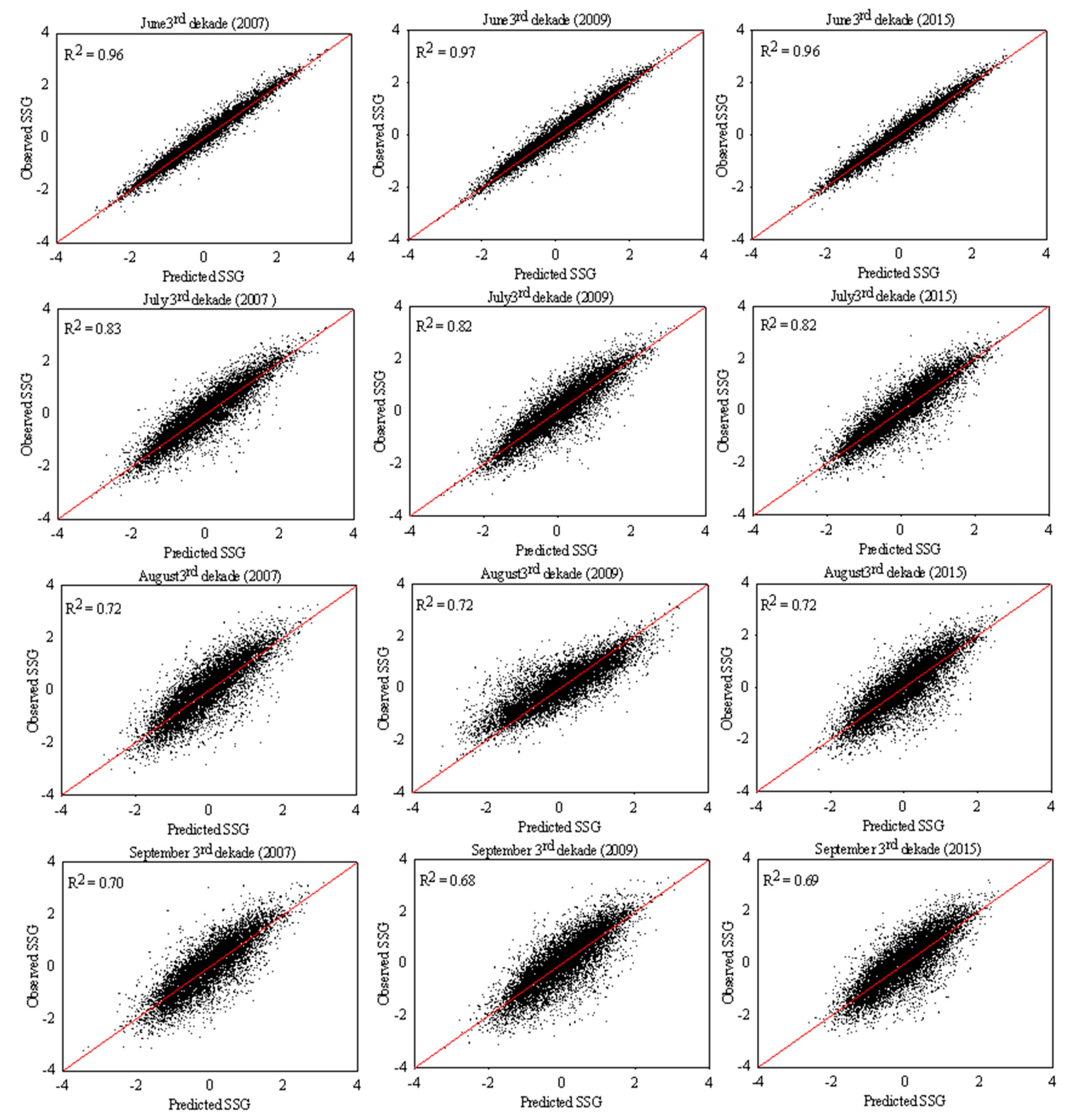
3.1. VegOut-UBN Model Prediction Accuracy

Figure 3 shows the prediction accuracy of the VegOut-UBN model measured in terms of the coefficient of determination (R²) and relative error (RE) of the observed and predicted SSG. The one-year data holding approach (Section 2.5) was used to train and to test the VegOut-UBN model. The models were developed for all dekades; however, the resulting graphs obtained for the last dekades of June, July, August, and September are presented for demonstration and further discussion (Figure 3). In general, the performance of the VegOut-UBN model is reasonably accurate (R² > 0.65, RE < 0.5) in predicting the vegetation outlook up to the end of the growing season during the model construction period (Figure 3a). The model performance during the test period (Figure 3a’) is relatively lower than that of the training models. A possible explanation for the lower accuracy of the test cases could be the shorter data length (only one year of test data for the holdout year) as compared to the training data length (15 years) used for the models’ construction. The model prediction accuracy decreases as the prediction length increases during both the model construction and test periods. A minimum relative error (RE < 0.6) was obtained during model construction and test cases (RE close to 0.6), which shows the good performance of the model in predicting VegOut-UBN. Similarly, the relative error shows increasing magnitude with increases in the prediction length during both the model construction and test cases.

Figure 4 shows the scatter plot of the observed and predicted SSG during model construction (training period) for the selected third dekades of June, July, August, and September. These dekades were selected to evaluate the model accuracy at the end of each month across the growing seasons of 2007, 2009, and 2015. The figure shows that the points cluster closely toward the imaginary line (45° trend line) for shorter prediction length (June 3rd dekade) and scatter out of the imaginary line when the prediction length increases. For example, a maximum R² value (0.97) and least spread of the scatter point were observed for the June 3rd dekade model whereas the minimum R² value (0.68) and relatively dispersed scatter points were observed for the September 3rd dekade model. The minimum R² value of the September 3rd dekade model satisfies the good model performance criterion (R² > 0.6). This depicts a strong agreement between the observed and predicted SSG, which proves the best performance of the VegOut-UBN model.

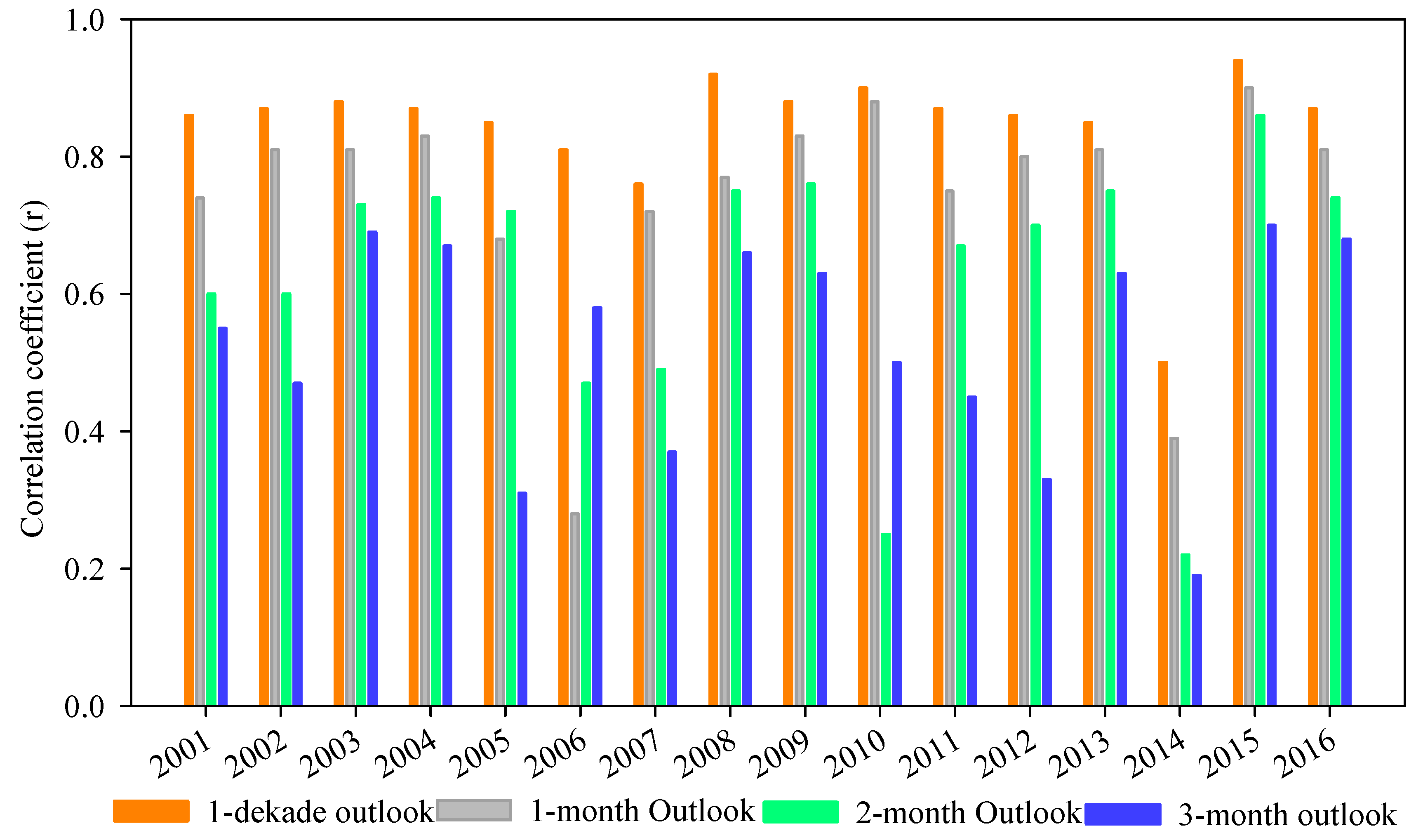
3.2. Spatial Pattern Correlation

The spatial pattern recognition of the observed SSG against the model-estimated outlook map was developed for each year, as shown in Figure 5. The resulting correlation coefficient (r) shows a decreasing trend for an increase in the outlook leading time. For example, the average correlation coefficient value for the one-dekade outlook is ~0.84; the values showed a decreasing trend for the one-month outlook (~0.73), two-month outlook (~0.62), and three-month outlook (~0.54). This shows that the best performance of the model is often observed in predicting the vegetation outlook at a shorter leading time. Moreover, the model displayed relatively better performance during drought years compared to normal or wet years. The year 2015 is known for a severe drought that covered most of the country. The dryness of this year is shown in this study and a maximum spatial correlation value is observed for all the outlooks. A similar result was observed for other historic drought events in the basin (2003, 2008, and 2009). The model shows a less satisfactory performance in predicting the vegetation condition during the normal years (2006, 2007, and 2014).

3.3. Spatial Patterns of VegOut-UBN Across the Region

The spatial patterns of one-dekade, one-month, two-month, and three-month vegetation outlooks as forecast on June 1st dekade (1–10 June) for the selected wet year (2007) and drought years (2009 and 2015) are shown in Figure 6. The droughts of 2009 and 2015 were selected to demonstrate the VegOut-UBN model performance using retrospective analysis of the vegetation conditions with the observed satellite-derived vegetation (SSG) for the same dekade in the growing season. These years were reported as some of the worst drought years in Ethiopia, when more than 10.1 million people were in need of food aid (OCHA 2016). In general, the VegOut-UBN model showed strong prediction capability of the vegetation condition at lower prediction periods (e.g., one dekade, one month) for both drought and wet conditions. The prediction accuracy decreased as the prediction period increased (e.g., two months, three months). In Figure 6, three categories (“overpredicted” for values greater than 1, “similar” for values between 1 and −1 inclusive, and “underpredicted” for values less than −1) were used to indicate the significant difference between the predicted and observed SSG in the difference map. Underprediction of the SSG values was observed in the eastern part and overprediction was observed in most of the central and southern areas of the basin during the wet year (2007). Similarly, underprediction of the vegetation stress (drought condition) in 2009 was observed in the eastern part and some pockets of the southern and central parts of the basin, whereas overprediction of the vegetation condition was observed in in the majority of the basin. The vegetation stress in 2015 in the eastern part and some pockets of the southeastern and southern parts of the basin was captured by the VegOut-UBN model for two- and three-month predictions in the majority of the basin, except in some pockets in the northwestern and eastern parts that showed good vegetation condition contrary to the observed SSG. Although overestimation and underestimation of the VegOut model were observed for the wet and drought years, respectively, the model could be used in supporting the decision-making process for mitigating and preparing for future drought events.

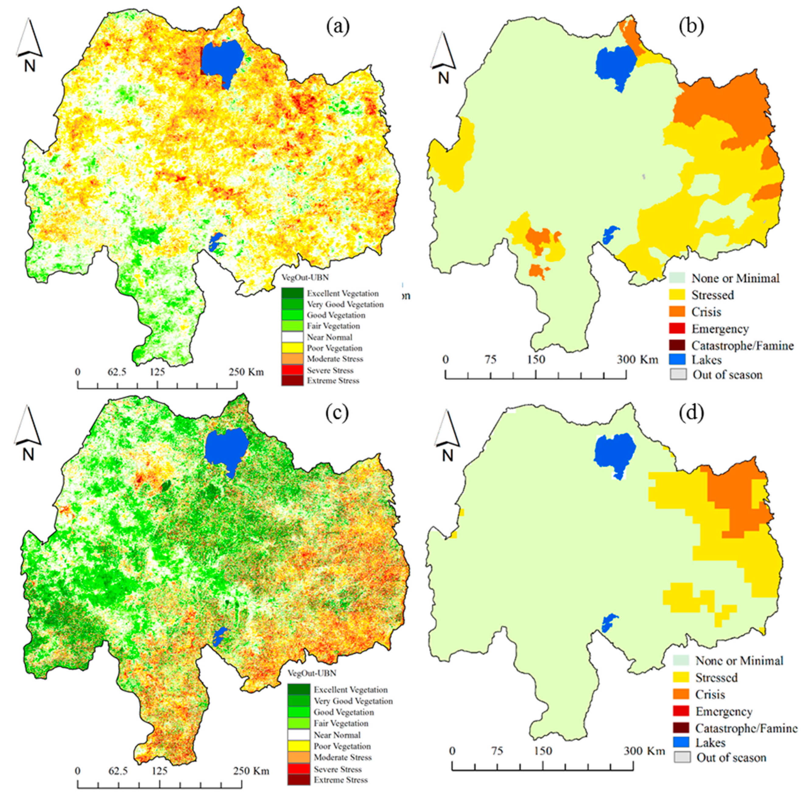
3.4. Comparison Result of VegOut-UBN Model with SPI and Food Security Maps

The VegOut-UBN model was compared with measured rainfall data for the selected 14 meteorological stations that are uniformly distributed across the UBN basin (Figure 1). The time series of the SPI values for the aggregate periods of 1, 3, 6, 9, 12, 24, and 60 months were used to compare with the VegOut-UBN model. Figure 7 shows the correlation coefficient results between VegOut-UBN and SPI for several aggregate periods. The result shows good agreement between VegOut-UBN and SPI with a correlation coefficient value of greater than 0.5 in most of the stations. Good correlation coefficient values (>0.5) were observed in Ghimbi and Gidayana stations for all the aggregate periods. Relatively good agreement was observed between VegOut-UBN and SPI at the 9-month aggregate period in most of the stations. The SPI for the 24- and 60-month aggregate periods also showed a good correlation in some of the stations. Therefore, a thorough study should be undertaken to identify the SPI aggregate period that would correlate best with the VegOut-UBN model. The lack of strong correlation coefficient values in most of the stations indicates that the VegOut-UBN model is influenced by several variables, including rainfall.

Another effort was also made to evaluate and compare the VegOut-UBN model with the food security situation map for July to September of 2009 and 2015. The years 2009 and 2015 were selected for this evaluation because of the availability of the food security status data. The average VegOut-UBN map for July to September (Figure 8a,c) was considered and compared with the food security status map (Figure 8b,d) of the same period. The result shows that the eastern part of the basin is often associated with poor vegetation condition (Figure 8a,c) and less food-secure regions (Figure 8b,d). Extended food-insecure areas were observed in 2009 compared to 2015. Similarly, VegOut-UBN also showed larger areas of poor vegetation condition in 2009 compared to 2015, reflecting the severity of the drought condition in 2009. In the central and northwestern parts of the basin, VegOut-UBN showed poor vegetation conditions, whereas the food security map showed “None or Minimal” in 2009. To the contrary, the food security map showed “stressed to critical” in the south central part while VegOut showed good vegetation condition. In 2015, VegOut-UBN showed good vegetation condition (no drought condition) in most parts of the basin that was supported by a “None or Minimal” food security situation. However, the southern parts and some pockets in the northwestern parts of the basin showed vegetation stress (drought condition), whereas “None or Minimal” food security status was observed. The reason for the opposite result observed in these parts of the basin needs further investigation in our future studies. The comparison result of VegOut-UBN with the food security status highlights the potential application of VegOut-UBN for indicating the food security situation for certain lead times.

The average values of the VegOut-UBN for the reference food security status regions of FEWSNET were extracted to qualitatively assess the drought severity ranges in these regions.

Table 4. Average VegOut-UBN values for different categories of food security status in 2009 and 2015.

Food Security Status	Average VegOut-UBN Values
	2009	2015
None or Minimal	−0.23	0.14
Stressed	−0.41	−0.31
Crisis	−0.54	−0.39

shows the average VegOut-UBN values for “none or minimal”, “stresses”, and “crisis” food security status for 2009 and 2015. The results show that relatively minimal negative VegOut-UBN values (reflecting drought conditions) were observed during “crisis” compared to “stress” and “minimal” food security status regions for 2009 and 2015. This indicates a strong linkage between drought and food security in Ethiopia. Hence, the VegOut-UBN can potentially be used to monitor and provide early warning in identifying food-insecure regions for the basin.

4. Conclusions

In this study, a VegOut-UBN model was developed for the UBN basin through integrating several input variables representing the different components of the hydrological cycle. The rule-based regression tree data mining approach was adapted to develop a VegOut-UBN prediction model that could potentially be used to monitor and mitigate the adverse impacts of drought. Such a drought model is still lacking for the UBN basin, which is commonly regarded as the main source of water for the main Nile River; the drainage basin of the Nile River covers eleven riparian countries. VegOut-UBN characterizes the level of drought stress on the vegetation condition and predicts the level of the vegetation condition for several leading times at relatively finer spatial and temporal resolutions. After analyzing the results, the following main conclusions were drawn.

The VegOut-UBN model has shown its capability in predicting the vegetation condition for certain leading times; therefore, the model can potentially be used as a good drought monitoring and early warning system for the basin. The comparison results of the VegOut-UBN model with the food security status map highlighted the potential application of the VegOut-UBN model for developing the food security outlook for the basin. VegOut-UBN can be used as a potential tool in supporting informative decision-making processes by different stakeholders, governmental and non-governmental organizations and institutions, in order to combat and prepare for future drought. The evaluation of VegOut-UBN with the SPI showed a lack of strong correlation coefficient values for most of the stations, which indicates that the VegOut-UBN model is influenced not only by rainfall but also by several other input variables.

References

1. Block, S.A. Agriculture and economic growth in Ethiopia: Growth multipliers from a four-sector simulation model. Agric. Econ. 1999, 20, 241–252. [Google Scholar] [CrossRef]
2. Diao, X.; Hazell, P.; Thurlow, J. The role of agriculture in African development. World Dev. 2010, 38, 1375–1383. [Google Scholar] [CrossRef]
3. IFPRI (International Food Policy Research Institute). Available online: http://www.ifpri.org/blog/ethiopias-2015-drought-no-reason-famine (accessed on 24 June 2017).
4. OCHA. Available online: http://reliefweb.int/sites/reliefweb.int/files/resources/START-briefing-Ethiopia-Jan-2016.pdf (accessed on 20 June 2017).
5. Viste, E.; Korecha, D.; Sorteberg, A. Recent drought and precipitation tendencies in Ethiopia. Theor. Appl. Climatol. 2013, 112, 535–551. [Google Scholar] [CrossRef]
6. Bayissa, Y.; Semu, A.; Yunqing, X.; Schalk, A.; Shreedhar, M.; Dimitri, S.; Griensven, A.; Tadesse, T. Spatio-temporal assessment of meteorological drought under the influence of varying record length: The case of Upper Blue Nile Basin, Ethiopia. Hydrol. Sci. J. 2015, 60, 1927–1942. [Google Scholar] [CrossRef]
7. Tadesse, T.; Wardlow, B.D.; Svoboda, M.D.; Hayes, M.J. Vegetation Outlook (VegOut): Predicting Remote Sensing–Based Seasonal Greenness. In Remote Sensing of Drought: Innovative Monitoring Approaches; CRC Press: Boca Raton, FL, USA, 2012. [Google Scholar]
8. Verdin, J.; Klaver, R. Grid-cell-based crop water accounting for the famine early warning system. Hydrol. Process 2002, 16, 1617–1630. [Google Scholar] [CrossRef]
9. Funk, C.; Peterson, P.; Landsfeld, M.; Pedreros, D.; Verdin, J.; Rowland, J.; Romero, B.; Husak, G.; Michaelsen, J.; Verdin, A.; et al. A Quasi-Global Precipitation Time Series for Drought Monitoring. US Geol. Surv. Data Ser. 2014, 832. [Google Scholar] [CrossRef]
10. Ji, L.; Peters, A.J. Assessing vegetation response to drought in the northern Great Plains using vegetation and drought indices. Remote Sens. Environ. 2003, 87, 85–98. [Google Scholar] [CrossRef]
11. Liu, W.T.; Kogan, F.N. Monitoring regional drought using the vegetation condition index. Int. J. Remote Sens. 1996, 17, 2761–2782. [Google Scholar] [CrossRef]
12. Westphal, C.; Blaxton, T. Data Mining Solutions: Methods and Tools for Solving Real-World Problems; John Wiley & Sons: New York, NY, USA, 1998. [Google Scholar]
13. Brown, J.F.; Wardlow, B.D.; Tadesse, T.; Hayes, M.J.; Reed, B.C. The vegetation drought response index (VegDRI): A new integrated approach for monitoring drought stress in vegetation. GISci. Remote Sens. 2008, 45, 16–46. [Google Scholar] [CrossRef]
14. Seleshi, Y.; Demaree, G.R. Rainfall variability in the Ethiopian and Eritrean highlands and its links with the Southern Oscillation Index. J. Biogeogr. 1995, 2, 945–952. [Google Scholar] [CrossRef]
15. Bayissa, Y.; Tadesse, T.; Demisse, G.; Shiferaw, A. Evaluation of satellite-based rainfall estimates and application to monitor meteorological drought for the Upper Blue Nile Basin, Ethiopia. Remote Sens. 2017, 9, 669. [Google Scholar] [CrossRef]
16. AghaKouchak, A.; Farahmand, A.; Melton, F.S.; Teixeira, J.; Anderson, M.C.; Wardlow, B.D.; Hain, C.R. Remote sensing of drought: Progress, challenges and opportunities. Rev. Geophys. 2015, 53, 452–480. [Google Scholar] [CrossRef] [Green Version]
17. Tucker, C.J.; Choudhury, B.J. Satellite remote sensing of drought conditions. Remote Sens. Environ. 1987, 23, 243–251. [Google Scholar] [CrossRef]
18. Han, J.; Pei, J.; Kamber, M. Data Mining: Concepts and Techniques; Elsevier: Amsterdam, The Netherlands, 2011. [Google Scholar]
19. Zheng, H.; Chen, L.; Han, X.; Zhao, X.; Ma, Y. Classification and regression tree (CART) for analysis of soybean yield variability among fields in Northeast China: The importance of phosphorus application rates under drought conditions. Agric. Ecosyst. Environ. 2009, 132, 98–105. [Google Scholar] [CrossRef] [Green Version]
20. Tadesse, T.; Wilhite, D.A.; Hayes, M.J.; Harms, S.K.; Goddard, S. Discovering associations between climatic and oceanic parameters to monitor drought in Nebraska using data-mining techniques. J. Clim. 2005, 18, 1541–1550. [Google Scholar] [CrossRef]
21. Tadesse, T.; Wardlow, B.D.; Hayes, M.J.; Svoboda, M.D.; Brown, J.F. The Vegetation Outlook (VegOut): A new method for predicting vegetation seasonal greenness. GISci. Remote Sens. 2010, 47, 25–52. [Google Scholar] [CrossRef]
22. Tadesse, T.; Demisse, G.B.; Zaitchik, B.; Dinku, T. Satellite-based hybrid drought monitoring tool for prediction of vegetation condition in Eastern Africa: A case study for Ethiopia. Water Resour. Res. 2014, 50, 2176–2190. [Google Scholar] [CrossRef] [Green Version]
23. Tadesse, T.; Wilhite, D.A.; Harms, S.K.; Hayes, M.J.; Goddard, S. Drought monitoring using data mining techniques: A case study for Nebraska, USA. Nat. Hazards 2004, 33, 137–159. [Google Scholar] [CrossRef]
24. Panda, S.S.; Ames, D.P.; Panigrahi, S. Application of vegetation indices for agricultural crop yield prediction using neural network techniques. Remote Sens. 2010, 2, 673–696. [Google Scholar] [CrossRef]
25. Tadesse, T.; Champagne, C.; Wardlow, B.D.; Hadwen, T.A.; Brown, J.F.; Demisse, G.B.; Bayissa, Y.A.; Davidson, A.M. Building the vegetation drought response index for Canada (VegDRI-Canada) to monitor agricultural drought: First results. GISci. Remote Sens. 2017, 54, 230–257. [Google Scholar] [CrossRef]
26. Chen, C.S.; Chen, W.C.; Chen, Y.L.; Lin, P.L.; Lai, H.C. Investigation of orographic effects on two heavy rainfall events over southwestern Taiwan during the Mei-yu season. Atmos. Res. 2005, 73, 101–130. [Google Scholar] [CrossRef]
27. Conway, D. The climate and hydrology of the Upper Blue Nile River. Geogr. J. 2000, 166, 49–62. [Google Scholar] [CrossRef]
28. Kebede, S.; Travi, Y.; Alemayehu, T.; Marc, V. Water balance of Lake Tana and its sensitivity to fluctuations in rainfall, Blue Nile basin, Ethiopia. J. Hydrol. 2006, 316, 233–247. [Google Scholar] [CrossRef]
29. Yilma, A.D.; Awulachew, S.B. Characterization and atlas of the Blue Nile Basin and its sub basins. In Proceedings of the International Water Management Institute (IWMI), Colombo, Sri Lanka, 5–6 February 2009. [Google Scholar]
30. Mellander, P.E.; Gebrehiwot, S.G.; Gärdenäs, A.I.; Bewket, W.; Bishop, K. Summer rains and dry seasons in the Upper Blue Nile Basin: The predictability of half a century of past and future spatiotemporal patterns. PLoS ONE 2013, 8, e68461. [Google Scholar] [CrossRef] [PubMed]
31. Degefu, M.A.; Rowell, D.P.; Bewket, W. Teleconnections between Ethiopian rainfall variability and global SSTs: Observations and methods for model evaluation. Meteorol. Atmos. Phys. 2017, 129, 173–186. [Google Scholar] [CrossRef]
32. Tekleab, S.; Mohamed, Y.; Uhlenbrook, S. Hydro-climatic trends in the Abay/Upper Blue Nile basin, Ethiopia. Phys. Chem. Earth Parts A/B/C 2013, 61, 32–42. [Google Scholar] [CrossRef]
33. TECSULT: Ethiopian Energy II Project. Woody Biomass Inventory and Strategic Project (WBISPP)–Phase 2 –Terminal Report; Ministry of Agriculture: Addis Ababa, Ethiopia, 2004.
34. Betrie, G.D.; Mohamed, Y.A.; van Griensven, A.; Srinivasan, R. Sediment management modelling in the Blue Nile Basin using SWAT model. Hydrol. Earth Syst. Sci. 2011, 15, 807–818. [Google Scholar] [CrossRef] [Green Version]
35. McKee, T.B.; Doesken, N.J.; Kleist, J.; American Meteorological Society. Drought monitoring with multiple time scales. In Proceedings of the 9th Conference on Applied Climatology, Dallas, TX, USA, 15–20 January 1995; pp. 233–236. [Google Scholar]
36. Gissila, T.; Black, E.; Grimes, D.I.F.; Slingo, J.M. Seasonal forecasting of the Ethiopian summer rains. Int. J. Climatol. 2004, 24, 1345–1358. [Google Scholar] [CrossRef] [Green Version]
37. Korecha, D.; Barnston, A.G. Predictability of June–September rainfall in Ethiopia. Mon. Weather. Rev. 2007, 135, 628–650. [Google Scholar] [CrossRef]
38. Camberlin, P.; Janicot, S.; Poccard, I. Seasonality and atmospheric dynamics of the teleconnection between African rainfall and tropical sea-surface temperature: Atlantic vs. ENSO. Int. J. Climatol. 2001, 21, 973–1005. [Google Scholar] [CrossRef] [Green Version]
39. Degefu, W. Some aspects of meteorological droughts in Ethiopia. In Drought Hunger in Africa; Glantz, M.H., Ed.; Cambridge University Press: Cambridge, UK, 1987; pp. 23–36. [Google Scholar]
40. ESRL. Available online: https://www.esrl.noaa.gov/psd/data/climateindices/list/ (accessed on 23 June 2017).
41. Batjes, N.H. Harmonized soil profile data for applications at global and continental scales: Updates to the WISE database. Soil Use Manag. 2009, 25, 124–127. [Google Scholar] [CrossRef]
42. Xia, Y.; Ek, M.B.; Wu, Y.; Ford, T.; Quiring, S.M. Comparison of NLDAS-2 simulated and NASMD observed daily soil moisture. Part I: Comparison and analysis. J. Hydrometeorol. 2015, 16, 1962–1980. [Google Scholar] [CrossRef]
43. Rulequest. An Overview of Cubist; RuleQuest Research Pty Ltd.: St Ives, NSW, Australia, 2013; Available online: https://www.rulequest.com/cubist-win.html (accessed on 20 June 2017).
44. Rajput, A.; Soni, R.; Aharwal, R.P.; Sharma, R. Impact of data mining in drought monitoring. IJCSI Int. J. Comput. Sci. 2011, 6, 309. [Google Scholar]
45. McKee, T.B.; Doesken, N.J.; Kleist, J. The relationship of drought frequency and duration to time scales. In Proceedings of the 8th Conference on Applied Climatology, Anaheim, CA, USA, 17–22 January 1993; pp. 179–184. [Google Scholar]
46. Bayissa, Y.A.; Tadesse, T.; Svoboda, M.; Wardlow, B.; Poulsen, C.; Swigart, J.; Van Andel, S.J. Developing a satellite-based combined drought indicator to monitor agricultural drought: A case study for Ethiopia. GISci. Remote Sens. 2018, 1–31. [Google Scholar] [CrossRef]
47. Bayissa, Y.A.; Maskey, S.; Tadesse, T.; van Andel, S.J.; Moges, S.; van Griensven, A.; Solomatine, D. Comparison of the performance of six drought índices in characterizing historical drought for the Upper Blue Nile Basin, Ethiopia. Geosciences 2018, 8, 81. [Google Scholar] [CrossRef]
Figure 1. The location, elevation, and boundary of the Upper Blue Nile (UBN) Basin (bold dark violet color). The red circles indicate the locations of the meteorological stations used to validate the VegOut-UBN model.
Remotesensing 11 00371 g001
Figure 2. The summary flow chart that shows the method followed in this study.
Remotesensing 11 00371 g002
Figure 3. The prediction accuracy of the VegOut-UBN model using the coefficient of determination (R2) and relative error (RE) for the selected dekades across the growing season. We used a one-year data holding approach during model construction (graphs on the left) and to test the model (graphs on the right).
Remotesensing 11 00371 g003
Figure 4. Scatterplots of observed and predicted SSG values during model constructions (training cases) for the last dekades of June, July, August, and September. These scatter plots were produced by holding out the data of 2007 (left), 2009 (middle), and 2015 (right).
Remotesensing 11 00371 g004
Figure 5. The spatial correlation coefficient values between the VegOut-UBN and observed SSG for different outlooks for 2001–2016.
Remotesensing 11 00371 g005
Figure 6. VegOut-UBN outlook, observed SSG, and difference maps for the selected normal year (2007, Figure 6A) and historic droughts (2009, Figure 6B, and 2015, Figure 6C) In the legend of the difference map, “Underpredicted” represents SSG values less than −1, “Similar” represents SSG values between 1 and −1 inclusive, and “Overpredicted” represents SSG values greater than 1.
Remotesensing 11 00371 g006
Figure 7. The correlation coefficient graph of the VegOut-UBN and SPI (different aggregate periods) for the selected meteorological stations.
Remotesensing 11 00371 g007
Figure 8. Average VegOut-UBN for July to September 2009 (a) and 2015 (c) and food security situation for July to September 2009 (b) and 2015 (d) according to United States Agency for International Development (USAID) and the Famine Early Warning Systems Network (FEWSNET, 2015).
Remotesensing 11 00371 g008