Abstract
Designing a sampling strategy for soil property mapping from remote sensing imagery entails making decisions about sampling pattern and number of samples. A consistent number of ancillary data strongly related to the target variable allows applying a sampling strategy that optimally covers the feature space. This study aims at evaluating the capability of multispectral (Sentinel-2) and hyperspectral (EnMAP) satellite data to select the sampling locations in order to collect a calibration dataset for multivariate statistical modelling of the Soil Organic Carbon (SOC) content in the topsoil of croplands. We tested different sampling strategies based on the feature space, where the ancillary data are the spectral bands of the Sentinel-2 and of simulated EnMAP satellite data acquired in Demmin (north-east Germany). Some selection algorithms require setting the number of samples in advance (random, Kennard-Stones and conditioned Latin Hypercube algorithms) where others automatically provide the ideal number of samples (Puchwein, SELECT and Puchwein+SELECT algorithm). The SOC content and the spectra extracted at the sampling locations were used to build random forest (RF) models. We evaluated the accuracy of the RF estimation models on an independent dataset. The lowest Sentinel-2 normalized root mean square error (nRMSE) for the validation set was obtained using Puchwein (nRMSE: 8.7%), and Kennard-Stones (9.2%) algorithms. The most efficient sampling strategies, expressed as the ratio between accuracy and number of samples per hectare, were obtained using Puchwein with EnMAP and Puchwein+SELECT algorithm with Sentinel-2 data. Hence, Sentinel-2 and EnMAP data can be exploited to build a reliable calibration dataset for SOC mapping. For EnMAP, the different selection algorithms provided very similar results. On the other hand, using Puchwein and Kennard-Stones algorithms, Sentinel-2 provided a more accurate estimation than the EnMAP. The calibration datasets provided by EnMAP data provided lower SOC variability and lower prediction accuracy compared to Sentinel-2. This was probably due to EnMAP coarser spatial resolution (30 m) less adequate for linkage to the sampling performed at 10 m scale.
1. Introduction
Remote sensing data are widely used for soil mapping, because they allow coveringlarge area in a cost effectiveway. However, an accurate soil sampling within the investigated area is necessary to produce soil variable or soil classification maps. The choice of the sampling strategy has great importance for soil mapping accuracy and the error caused by an unrepresentative sampling dataset could be larger than the analytical error associated to laboratory measurements [1]. The sampling strategy entails making decisions about sampling pattern, sample size and sampling location. A suitable sampling strategy allows building a reliable calibration dataset, which in turn allows carrying out a prediction model that produces precision maps of the target variable. Two main sampling strategies exist: design-based and model based approach [2]. The design-based approach is based on the probability theory and it assumes that data are independent. Nevertheless, soil and geological data show a spatial dependence, i.e., the variance between values increases with distance. For this reason, a model-based sampling is the preferred strategy for Earth science applications, in other words an approach based on a geostatistical analysis. However, the model-based approach can be applied only if the parameters describing the spatial variability are already a priori known. Thus, if no legacy data exists, the parameters to build a variogram can only be obtained by sampling [3]. Alternatively, when the target data are not or to a limited extent available, the model-based approach can exploit the relationship between the target variable and ancillary data [4]. The availability of a consistent number of ancillary data (or covariates) allows applying sampling strategies according to the feature space and not based on the geographical space [5,6]. The covariate data points represent points in the feature space and are enclosed by a hypercube. Thus in this case the sampling design aims an optimization in feature space, which becomes more important than the spatial coverage, and usually leads to spatial clustering of the sample locations [7]. Provided that the covariates are strongly related to the target variable, the sampling strategy based on feature space can ensure a calibration dataset covering the range of the target values [8]. Some authors discussed the relative importance of the spatial and feature space coverage for providing reliable inputs for prediction models for soil or environmental variables [5,6,7]. Most of them suggested a compromise between feature and geographical space. Still, the choice of the sampling strategy depends on the goals of the study, the availability of legacy and ancillary data and the available budget [9]. In general, for sampling strategies based on the geographical space (e.g., grid sampling), a large number of samples for the calibration dataset (high sampling density) ensures a good precision albeit at higher costs. Consequently, during the sampling planning, it is necessary to find a compromise between precision and costs, and in particular, to choose the sampling strategy that ensures the lowest estimation error [10]. Strategies based on the feature space generally entail more clustered samples distribution, which in turn could reduce the efforts in the field, the travel costs and the number of samples. For these purposes, remote sensing data cheaply provide covariates over large areas. The physical link between spectral data in the optical domain and soil properties exists [11] and is widely exploited in a remote sensing context (e.g., [12]). Some absorption features are quite broad and they can partly overlap with spectral region related to a different soil property. For this reason, it is desirable using the whole spectrum as covariates instead of a single band or a narrow region. For example, the absorption features related to clay minerals are mainly located in the short wave infrared (SWIR) region. However, each clay mineral shows narrow absorbance peaks at specific wavelengths [11,13]. Since only rarely a single clay mineral is present in the soil, the quantitative estimation of clay content uses all spectral data having good signal quality. Similarly, Soil Organic Carbon (SOC) prediction models exploit most of the spectral regions across the electromagnetic spectrum between 400 and 2500 nm [14,15] and this is due to the large heterogeneity of the components of the organic matter. So given the link between spectral characteristics and soil variability, the absorbance/reflectance values at a given wavelength can be considered as covariates related to the target variable and consequently the spectral variability can be exploited for sampling strategies based on feature space. Many algorithms exploit spectral data to obtain a calibration dataset that includes the spectral variability of a population (e.g., Kennard–Stones algorithm). Most of these algorithms were successfully tested on soil spectra acquired in the laboratory [16] or in the field [17]. However, to our knowledge, soil spectra acquired by airborne or satellite sensors were never exploited for a sampling selection algorithm.
Spectra of bare soils in cropland fields are widely available as the two Sentinel-2 satellites ensure a short revisit time (5 days). Therefore, soil spectra can be first exploited to set the sampling strategy and then, after sampling and laboratory analysis of the desired soil property, as predictors for the target variables. The same sampling strategy could in the future be used for analysing the spectra from hyperspectral satellite sensors when they become available. However, although the forthcoming hyperspectral satellite sensors will provide data over a large spectral range and with narrow bandwidths, the spatial resolution will be generally lower than that provided by Sentinel-2. Both the German Environmental Mapping and Analysis Program (EnMAP) [18] and the Italian PRecursoreIperSpettraledellaMissioneApplicativa (PRISMA) [19] sensor will acquire with a spatial resolution of 30 m, and this resolution may not be sufficient if the target soil property has a short-scale spatial variability. Moreover, in small fields bordering roads, built up areas or crops, the number of usable pixels could become very low, since the soil spectra extracted from the pixels along the borders are not pure, but the average among two or more materials (mixed pixels).
We aim evaluating the capability of multispectral (Sentinel-2) and hyperspectral (simulated EnMAP) satellite data to select the sampling locations in order to collect a calibration dataset that covers the SOC variability of the area. We tested different sampling strategies based on the feature spaces, where the ancillary data are the spectral bands of the Sentinel-2 and simulated EnMAP data from imagery acquired in north-east Germany. We tested both sampling selection algorithms requiring setting the number of sample in advance and others that automatically provide the ideal number of samples. The efficiency of the sampling selection was also evaluated in terms of prediction accuracy of the SOC maps.
2. Materials and Methods
2.1. Study Area
The study area is located around the municipality of Demmin in north-eastern Germany (Figure 1; 53°52′N; 13°13′E) and is part of the TERENO [20] north-eastern German lowland Observatory (TERENO-NE) from the Helmholtz Association. The mean temperature is 8 °C with an annual precipitation between 500 and 600 mm [21]. This area is mainly characterized by croplands with very large fields on glacial till, while grassland represents around 25% of the area and mainly occurs in the floodplains characterized by organic and shallow peat soils. The topography is rolling (mean relief ca. 120 m) to slightly hilly in the south. The spatial variability of soil types reflects the variation in parent material and relief. In the flat area around the town of Demmin, the soils are characterized by a sandy layer that entails a lower organic matter content as compared to the surrounding soils. Thus, the area can be divided into three main soil associations according to the Soil Map of the Federal Republic of Germany (1:1,000,000) [22]: (i) organic and shallow peat soils in the floodplains; (ii) clayey glacial till soils rich in organic matter, and (iii) sandy glacial till soils.
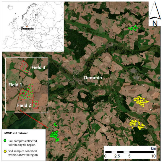
Figure 1.
RGB (red: 665 nm; green: 560 nm; blue: 490 nm) satellite image acquired by Sentinel-2 sensor of the study area with location of the soil samples of the Mecklenburg-West Pomerania (MWP) dataset.The white frame is a zoom of field 1, 2 and 3.
Samples were acquired from the upper soil layer (0–10 cm) within the clay glacial till and sandy glacial till area and are part of the Mecklenburg-West Pomerania (MWP) database [23,24] (Figure 1). The MWP dataset consists of 181 soil samples, each sample consisted of five sub-samples taken with a gouge auger collected from 0–10 cm depth within an area of 5 m radius. The total carbon of the air-dried and sieved soil samples was measured by dry combustion using a CN (carbon and nitrogen) analyser (VarioMax, ElementarGmbh, Hanau, Germany), then the SOC was obtained by subtracting the inorganic carbon (in the form of carbonates) that was determined by measuring the pressure of CO2 emitted after the addition of hydrochloric acid. The SOC values range from 6.0 to 194.6 g kg−1, with a mean value of 19.5 g kg−1 and a standard deviation of 26.4 g kg−1 (Figure 2).
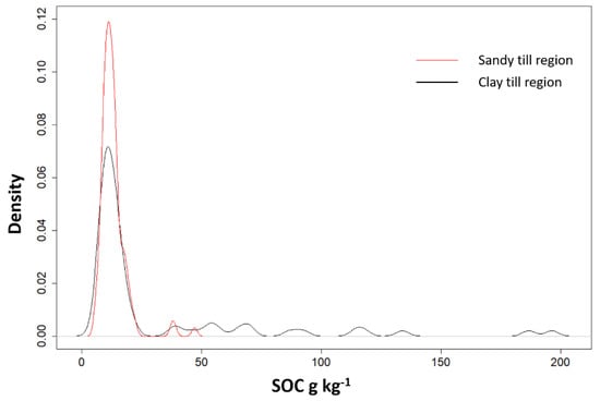
Figure 2.
Kernel density estimate plot for the measured Soil Organic Carbon (SOC) values of theMecklenburg-West Pomerania (MWP) dataset.
2.2. Remote Sensing Data
A cloud-free Sentinel-2 image acquired on 30 August 2018 (Figure 1), was downloaded from the Copernicus open access hub as Level-1C product. The Sentinel-2 sensors have 13 bands with different spatial resolution and bandwidth. We selected nine bands that are relevant for soil applications: B2 (490 nm), B3 (560 nm), B4 (665 nm), B5 (705 nm), B6 (740 nm), B7 (783 nm), B8 (842 nm), B11 (1610 nm) and B12 (2190 nm). The 20 m bands were spatially resampled to 10 m. The image was atmospherically corrected using the Sen2Cor processor (v. 2.5.5) [25], a plugin incorporated in the Sentinel Application Platform (SNAP) software, obtaining the Bottom of Atmosphere (BOA) reflectance.
Airborne images were acquired on 1 October 2015 with the HySpex system of the Helmholtz Center Potsdam GFZ, mounted on the Cessna 207T aircraft of the Free University of Berlin, part of the EnMAP science preparation program. The NEO HySpex system consists of two push-broom hyperspectral cameras (VNIR-1600 operating over the 400–1000 nm and SWIR 320m-e operating over 1000–2500 nm range) with a total of 416 wavebands and a spectral resolution of 3.7 nm (VNIR-1600) and 6.0 nm (SWIR-320m-e) (NorskElektroOptikk, 2017). From a mean altitude of 2500 m, the original ground sampling distance of the image was 1.9 m for the VNIR spectrometer and 4.0 m for the SWIR-320m-e camera, resampled to 4 m after data pre-processing. The pre-processing of the HySpex data to orthorectified reflectance was performed with the GFZ in-house processing chain HyPrepAir. First, geometric processing was performed, including co-registration and adaptation of the SWIR sensor to the VNIR [26]. Subsequently, atmospheric correction of the HySpex VNIR-SWIR data cube was applied with the ATCOR-4 software [27]. Then, a mosaicking of the single flight lines keeping the original data values was realized. Furthermore, an empirical line calibration was performed using ground measurements obtained simultaneous to flight acquisition to remove atmospheric attenuation and spectral artefacts. The airborne data were used to simulate an EnMAP image (Figure 3); the calculation of simulated EnMAP data and associated radiance and reflectance products (Level 1B/1C/2A) at 30 m spatial resolution was performed using the EnMAP end-to-end simulation software EeteS [28]. The EeteS software follows the forward and backward processing schemes simulating the EnMAP image generation process, sensor calibration and data pre-processing. The core payload of EnMAP consists of a dual-spectrometer instrument measuring in 242 spectral bands between 420 and 2450 nm with a spectral sampling distance varying between 5 and 12 nm. Next, the data were transformed to Level 1C applying a detector co-registration and image orthorectification, subsequently processed to reflectance orthorectified data (Level-2A) applying an atmospheric correction.
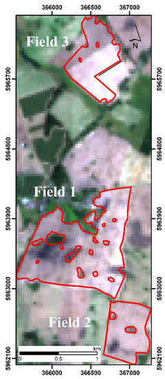
Figure 3.
EnMAP simulated image (red: 639.21 nm, green: 548.06 nm; blue: 459.59 nm) and the borders of the field 1, 2 and 3.
2.3. Preliminary Investigation
Soil spectra separated by large Euclidean or Mahalanobis distance are more different in terms of soil variables than two spectra separated by a smaller distance. However, in order to verify if the distance between spectra is directly correlated with the differences in terms of SOC content, we computed the mean Euclidian distance between the mean spectra of four subsets having different SOC levels based on the MWP dataset: <10 g kg−1, 10–12.2 g kg−1, 12.2–15.7 g kg−1, >15.7 g kg−1. The thresholdsbetween the four SOC classes were set according to the quartiles of the MWP dataset.
The spectra were obtained both from a Sentinel-2 and EnMAP simulated image at each sampling location. Before calculating the Euclidean distance, the EnMAP spectra were normalized (mean = 0 and variance = 1) using the standard normal variate transformation to reduce scattering effects.
The results showed a very high correlation coefficient (0.92) between the Euclidean distances and the differences in terms of SOC, both for Sentinel-2 and EnMAP data. Thus, these preliminary results suggest that the differences between spectra can be used to select soil samples that cover the variability in terms of SOC content in the study area.
2.4. Soil Sampling Strategies
All algorithms exploited a feature space based on a set of predictors or auxiliary variables. For each algorithm, the remote sensing spectra (Sentinel-2 or simulated EnMAP) were used as predictors (input matrix). The sample design was tested both at field and at regional scale. For the field tests, the spectra were extracted from all pixels within each field except the ones along the borders (distance <40 m). While for the regional applications, the matrix consisted of the spectra extracted at sampling points of the MWP dataset.
2.4.1. Selection Algorithms with a Predefined Sample size
As these algorithms require the number of samples to be setbeforehand, we set three different sample densities for each method: 0.4, 0.7 and 1 sample (s) per hectare.
The conditioned Latin Hypercube (cLHS) is a stratified random sampling procedure that exploits the multidimensional distribution provided by predictors (here the spectrarepresent the feature space and each spectral dimension equals one feature dimension). Thus, the algorithm aims to fully cover the feature space rather than the location space. This was done by dividing the multidimensional space into n strata and selecting one sample for each stratum. The complete description of the cLHS algorithm can be found in [6].
The Kennard-Stone algorithm (KS) selects n samples uniformly distributed over the predictor space from the entire dataset, thus optimizing the coverage of the spectral variability [29]. First, the algorithm finds the two samples that are furthest apart based on Euclidean distance assigning them to the calibration dataset and removing them from the input matrix. Then, the procedure is repeated until the number of the samples within the calibration dataset is equal to n.
Moreover, a random sampling selection (R) was tested, the random extraction was repeated 100 times for each of the three sampling densities.
2.4.2. Selection Algorithms Providing the Ideal Number of Samples
In contrast to the previous algorithms, the algorithms discussed in this section provide the ideal number of samples for a given dataset without predefining the sample density.However, their performance depends on some parameters linked to the Mahalanobis distance between spectra.
The Puchwein algorithm (PU) uses the Mahalanobis distance between spectra to iteratively eliminate similar samples and thus selecting only the most dissimilar spectra [30]. In the first step, the Puchwein algorithm performs a principal component analysis (PCA) on the input matrix. Then, the algorithm extracts the score matrix for a given number of principal components p. The score matrix is then normalized (mean = 0 and variance = 1) and the Mahalanobis distance between each spectrum and the centre of the data is computed. For the sample selection, the algorithm uses an initial limiting distance and then, it selects the sample X1 with the largest Mahalanobis distance to the centre. After that, the algorithm removes all samples having a distance equal to or smaller than the initial limiting distance from X1. Finally, the algorithm proceeds iteratively selecting X2, X3…Xn and removing each time the samples within the minimum distance from X. When there are no samples left in the dataset, the algorithm re-starts using an increased minimum distance. The Puchwein algorithm chooses the optimal selection of samples provided by the loop having the largest difference between the observed and theoretical sums of leverage. The initial limiting distance was set based on the formula k(p − 2), where k is usually 0.2 and p the number of components of the PCA for a given percentage of explained variance.
Similar to the Puchwein approach, the SELECT algorithm (SW) is also based on the Mahalanobis distance between samples [31], which is computed from the normalized score matrix obtained by PCA. This algorithm first selects the samples with the largest number of neighbours within a given minimum distance and removes them from the data set once they have been selected. The algorithm repeats the procedure until no samples are left.
In addition to the above-described algorithm, a combination of PU and SW was tested (PS). The sample selection was carried out in two steps: first, the PU algorithm selects n samples, then the n selected samples were further analysed by the SW algorithm, which selects a number of samples smaller than n.
The KS, PU and SW algorithms were computed using the Prospectr package in R [32], while we used the appropriate R package for the cLHSalgorithm R software [33].
2.5. Calibration and Validation of the Prediction Model
2.5.1. Field Tests
The SOC maps provided by [34] were obtained calibrating a Random forest (RF) regression model (RPD = 2.1), which exploited the SOC values at sampling points (analysedin the laboratory) and the Sentinel-2 spectral data. These SOC maps (10 m resolution) include fields 1, 2 and 3 (Table 1; Figure 4). Thus, after sample selection provided by each algorithm, the SOC content for each corresponding pixel was derived from the SOC maps. Then, the RF model was applied to all the bare soil fields of the Demmin area shown in Figure 1. The SOC values retrieved from S2 data were interpolated using block kriging with a block size of 30 m in order to obtain the same ground sample distance for the SOC maps and EnMAP data.

Table 1.
Descriptive statistics of the soil organic carbon content maps of the field 1, 2 and 3adapted from [34].
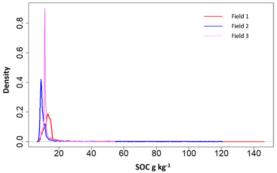
Figure 4.
Kernel density estimate plot for the SOC values of field 1, 2 and 3 adapted from [34].
The SOC values of the points provided by the selection algorithms and the bare soil spectra (Sentinel-2 or EnMAP) were used to build a calibration dataset, which was used to build a RF regression model (Figure 5). Since the SOC distribution is skewed, a Box-Cox transformation was carried out before runningeach RF model. The RF regression is a supervised learning algorithm, where all the decision trees make up the ‘forest’ [35]. The decision trees are combined through the resampled training dataset and the SOC values predicted by the RF regression are the mean values of the outputs of the regression trees. The RF regression method allows avoiding overfitting and reduces noise due to irrelevant features.
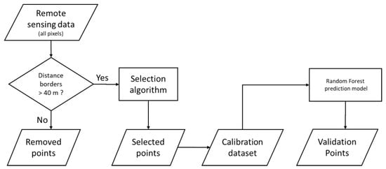
Figure 5.
Flow chart concerning sampling strategy and the validation of the prediction models.
The models were validated on 55 independent samples (42 samples from field1, 8 samples from field 2, 5 from field 3). These 55 samples of the validation dataset are part of the MWP dataset and were not used in the calibration dataset. Their SOC values range between 8.1 and 196.4 g kg−1, the mean value is 28.7 g kg−1 and the standard deviation is 41.9 g kg−1.
The estimation accuracy of the RF model was evaluated in terms of normalized root mean square error (nRMSE) and ratio of performance to deviation (RPD); Equations (1) and (2):
where is the observed SOC value, the SOC predicted by the RF model, std the standard deviation of the observed values and n the number of samples.
Moreover, the efficiency of the sampling dataset was evaluated for the tests with a RPD higher than 1.4 by a simple efficiency index (Ef) that is computed as the ratio of RPD to the number of samples (s) per hectare (Equation (3)):
2.5.2. Regional Tests
Since reliable SOC maps are not available in the sandy till region, we used all 181 samples of the MWB dataset for the regional tests (Figure 1). The Sentinel-2 spectra were divided into calibration (CAL) and validation (VAL) dataset based on the KS algorithm. The KS algorithm was set to select 130 samples (70%) for the CAL dataset. The remaining 51 samples (30%) are the VAL dataset. Then, each sample selection algorithm was tested on the CAL dataset, picking out the samples for the random forest model calibration. Finally, the model was verified on the VAL dataset. For the algorithms that do not provide the optimal number of samples (KS, R, and cLHS), we calibrated the RF model with n number of samples, where n increased from 10 to 130 in steps of 1. The estimation accuracy of the RF model was evaluated in terms of nRMSE and RPD.
3. Results
3.1. Validation at Field Scale
The sampling densities in the three fields correspond to 81(0.4 sample ha−1), 144 (0.7 sample ha−1) and 205 (1.0 sample ha−1) samples (Table 2). The SOC content of each calibration dataset is shown in the plots of Figure 6. Concerning the tests with Sentinel-2 data, the highest SOC validation accuracies were obtained using the highest density for all methodologies (Table 2). However, the largest Ef values were obtained with 0.7 s ha−1 for R (Ef = 2.1) and cLHS (Ef = 2.0) and using 0.4 s ha−1 for KS (Ef = 5.1). The PS algorithm selected only 26 samples (Figure 6c and Figure 7b) obtaining a nRMSEof 12% and the best efficiency value (Ef = 13.4). The highest RPD value was obtained using the PU method (RPD = 2.5; nRMSE = 8.7%). However, the number of samples for the calibration dataset was quite high (231; Figure 6c and Figure 7a) and consequently, the efficiency was low (Ef = 2.2). The EnMAP data at 30 m scale but with higher spectral resolution provided lower prediction accuracy as compared to the Sentinel-2 data, most of the RPD values were around 1.4, and the accuracy was generally low (Table 2). Based on the EnMAP data, the PU algorithm showed clearly the best performance with an RPD of 2.0, whereas all the other algorithms provided RPDs ~1.4–1.5. The EnMAP PU showed the highest Ef value (22.9) compared to the other algorithms and exploiting only 18 samples (Figure 6f and Figure 7c), thus a density of 0.1 s ha−1.
Table 2.
Descriptive statistics of the SOC content of the calibration datasets detected by the sampling selection algorithms in the three fields, and the estimation accuracy in terms of normalized root mean square error (nRMSE), ratio of the performance to deviation (RPD) and efficiency index (Ef) obtained from the validation dataset (R = random sampling selection, cLHS = conditioned Latin Hypercube; KS = Kennard-Stones; PU = Puchwein; SW = SELECT; PS = Puchwein+SELECT). The average and standard deviation nRMSE and RPD values were reported for the random sampling selection.
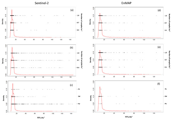
Figure 6.
Kernel density estimate plots for the SOC values (field 1, 2 and 3) for the Sentinel-2 (left side) and EnMAP (right side) data. The black circles represent the SOC content of the samples selected by the conditioned Latin hypercube (a,d) and the Kennard-Stones (b,e) algorithm for different sampling densities. The samples selected by the Puchwein (PU), SELECT (SW) and Puchwein+SELECT (PS) algorithms were shown at the bottom (c,f).
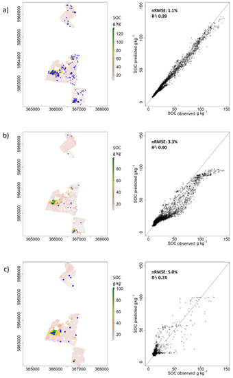
Figure 7.
The outputs obtained applying the Puchwein (a) and the Puchwein+SELECT (b) algorithm using the Sentinel-2 data, and those obtained using the Puchwein algorithm with EnMAP data (c). The location of the soil samples collected for the calibration datasetin the lefthand panels and the plot of observed against predicted SOC content for each pixel in the righthand panels.
Figure 7 shows the comparison between the SOC maps provided by [34] (SOC observed) and those obtained here (SOC predicted) with the PU and PS (only Sentinel-2) approach. The plot concerning the PU approach with Sentinel-2 data (Figure 7a) showed a high similarity between the two maps (nRMSE = 1.1% kg−1; R2 = 0.99), while the plot of the PS method (Figure 7b) highlighted a lower R2 value (0.90), which is in part due to the inability to predict SOC values larger than 90 g kg−1. The plot of the PU method with EnMAP data (Figure 7c) showsa fairly large spread of the points around the 1:1 line, which is reflected by much lower R2 (0.74) in comparison.
3.2. Validation at Regional Scale Based on Sentinel-2 Spectra
The CAL dataset consists of 130 samples, 51 of which collected in the clayey till region and 79 in the sandy till region (Table 3). Using all the 130 samples of the CAL dataset to build the RF, the nRMSE of validation was close to 9% and the RPD was 1.6. The random selection approach provided low prediction accuracy (RPD < 1.4) using less than 50 samples for the calibration model, then, increasing the number of samples, the RPD ranged between 1.4 and 1.6 (Figure 8). The maximum value was reached using 123 samples. The cLHS algorithm improved the prediction accuracy while reducing the number of samples as compared to the R strategy (Figure 9). The best SOC prediction accuracy with cLHSalgorithm was detected using 88 samples: 37 in the clay region and 51 in the sandy region (Figure 10b), ensuring a large range of SOC values (6–186.8 g kg−1) and a satisfactory RPD value (1.8). The KS algorithm provided very similar results to cLHS, both in term of selected samples (85) and RPD value (1.8). The highest RPD for PU algorithm was obtained selecting 34 samples (Figure 8 and Figure 9): only 14 samples in clay region and 20 in the sandy one (Figure 10d). The few selected samples were able to cover a large range of SOC values (7.8–196.4 g kg−1; Figure 9) and the RPD, be it lower than KS and cLHS, was still satisfactory (RPD = 1.6). The mean SOC value of the selected samples by PU algorithm was much higher (42.5 g kg−1) than the mean values of the datasets selected by SW, cLHS and KS algorithm (Table 3).
Table 3.
Descriptive statistics of the SOC content of the calibration datasets detected by the sampling selection algorithms at regional scale and the estimation accuracy in terms of normalized root mean square error (nRMSE), ratio of the performance to deviation (RPD) from the validation dataset. The number of selected samples within each soil association region: clay till (C_TILL) and Sandy till (S_TILL) are given.
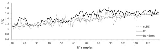
Figure 8.
Ratio of performance to deviation obtained using from 10 to 129 samples detected by random selection, conditioned Latin hypercube (cLHS) and Kennard-Stones (KS) algorithms.
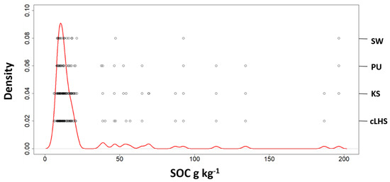
Figure 9.
Kernel density estimate plot for the SOC values of the CAL dataset. The circles indicate the SOC content of the samples selected by the Puchwein (PU), SELECT (SW), Kennard–Stones and conditioned Latin Hypercube (cLHS) algorithms.
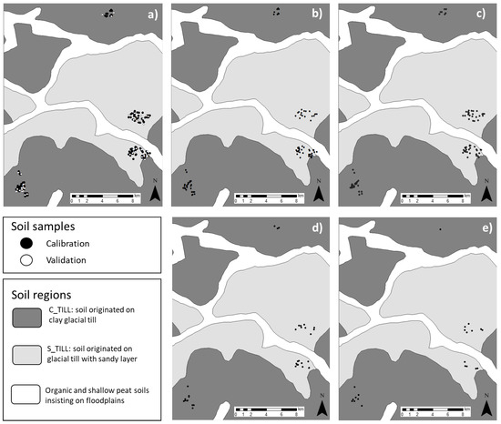
Figure 10.
Location of the samples of the MWP dataset (a) and those of the calibration dataset detected by the cLHS (b), Kennard–Stones (c), Puchwein (d) and SELECT (e) algorithms.
4. Discussion
Satellite images provide ancillary data over large areas, which can be useful for the spatial prediction of soil properties, especially when the information about the target variable is limited [6]. Ancillary data can also be successfully used for designing a sampling strategy [5]. Generally, sampling strategies based on the feature space (derived by ancillary data) provide better results than statistical and geometric approaches [9]. As most soil properties show spatial autocorrelation, a good spatial coverage exploiting the feature space can be obtained if the ancillary data are strongly related to the target variable and roughly on the same spatial autocorrelation level [6]. The results highlighted that the distance between spectra is directly correlated with the differences in terms of SOC content, meaning that it could be feasible to exploit both multispectral and hyperspectral data to select pixels having a wide SOC range. This is due to the large heterogeneity of the organic matter, which entails the absence of well-defined spectral features within a specific spectral region.Consequently, the wavelengths linked to the SOC content can be detected along the whole VNIR-SWIR (400–2500 nm) spectrum [14,15,36]. However, the assumption that larger spectral differences result in more different soil properties weakens if the spectral response of the target variable is mainly influenced by functional groups located in narrow spectral regions and not throughout the spectrum as for SOC. This could be the case, for example, for clay content that is strongly linked to absorption peaks in the SWIR region, which are associated to metal–OH bends and O–H stretch of the clay lattice [11,13]. Probably, in order to exploit spectral data for detecting as much clay variability as possible, the sample selection algorithms should be enhanced giving a different weight to the wavelengths affected by the absorption peaks.
As a general rule, the calibration dataset for empirical models should be representative for the range of values of the target variable. This avoids the need for extrapolation when applying the model for the prediction of the target variable. However, extreme samples in the spectral spaces could be outliers and not related to extreme SOC values [16]. In addition to the range, the calibration dataset should be representative of all the existing values across the range. This means that not only the extreme values must be present in the calibration dataset, but also the intermediate values, preserving a standard deviation of the target variable reflecting the one of the entire study area. Our results showed that increasing the standard deviation of the calibration datasets positively affects the accuracy of the SOC prediction models. In agreement with a previous study on exchangeable Ca+2 and clay content [16], we found a relationship between sample size and validation accuracy for the selection algorithms requiring to set the sample size (random, cLHS, KS), both at field and regional scale. However, often the cost for the field sampling and the laboratory measurements influences the sample size to a greater extent than the accuracy level [9]. Concerning the selection algorithms providing the optimal number of samples, no relationship between sample size and prediction accuracy was detected. For example, the PS algorithm yielded an RPD of 1.7 using only 26 samples for Sentinel-2 tests. In this case the standard deviation of the selected samplesis very high (35.5 g kg−1) and the selected samples are evenly distributed along the SOC range of the area (Figure 6c). An objective sampling selection without a priori information about the target variable enhances the precision of the prediction models while reducing the sampling and analysis costs. The SW algorithm has proven to be less conservative than PU concerning the SOC range due to a difference in selection procedure. The SW algorithm is based on the selection of samples having a large number of neighbours. Thus, the SW stratifies the feature space, followed by the selection of only one sample for each stratum. Although the removal of the neighbours selects few samples with large distances between them, the SW does not target samples with extreme values. Consequently, the calibration datasets selected by SW provided a narrower range as compared to the other algorithms (Figure 6c). The PU approach also stratifies removing the neighbours of the selected samples. However, the sample selection is based on the distance from the centre of the data. Thus, the PU algorithm allows the selection of more extreme values, which translates into larger range of SOC values both with Sentinel-2 and with EnMAP data. In order to find a good compromise between a reduced number of samples and an adequate SOC range and variability, we tested the PS algorithm. For the Sentinel-2 data, the SW algorithm further skimmed the number of samples detected by the PU method in the first step. The samples selected after the second step showed a SOC range slightly different to that obtained by PU. Nevertheless, the PS method appears to be particularly useful where the PU algorithm selects a large number of samples, while for the EnMAP and regional tests, the PS method selected aninsufficient number of spectra to calibrate a RF model (<10). Although PU, SW and PS provide the optimal number of samples, this number depends on the parameter setting. In particular, the selection of the initial Mahalanobis distance affects the number of samples selected by the PU algorithm.
All algorithms tested at the regional scale selected samples of the CAL dataset without oversampling one or the other of the two soil regions, thus respecting the proportions between C_TILL and S_TILL region. The C_TILL region includes loam and clay soil with a high SOC content, while the soils within the S_TILL region are usually sandy with a lower SOC content. These differences probably affect the spectral responses, allowing the algorithms to pick samples from both regions. In this regard, Figure 11 clearly shows how the 50% of S_TILL spectra are concentrated in the first quadrant of the PCA plot, while few C_TILL samples (8), characterised by low SOC values (6–11 g kg−1), can be observed in the same quadrant. The computational cost can be a restriction on the use of the sampling selection algorithms at regional scale. The processing of all the bare soil pixels within a Sentinel-2 or EnMAP image is time consuming and it needs powerful computers.
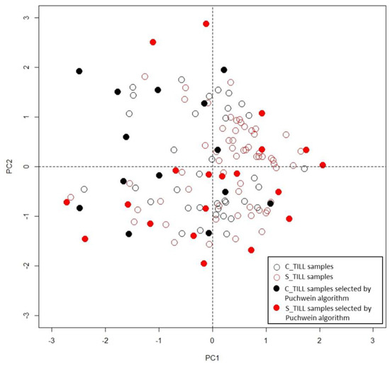
Figure 11.
First principal component against second principal component scores of the Sentinel-2 spectra of the CAL dataset.
Although EnMAP data have proven to successfully predict some soil properties exploiting the high spectral resolution of the sensor [37], the calibration datasets that were selected exploiting the EnMAP data generally provided low SOC variability and low prediction accuracy. The poorer results obtained by EnMAP as compared to Sentinel-2 are probably due to its coarser spatial resolution (30 m). Interestingly, a similar prediction accuracy between EnMAP and Sentinel-2 images was observed using the R and CLHS algorithms. On the other hand, KS and PU algorithms resulted in much higher prediction accuracy for the Sentinel-2 images. The spatial resolution of the Sentinel-2 SOC maps is 10 m and the soil samples were collected within an area of 5 m radius.Thus, the size of the sampling area is almost the same as the Sentinel-2 spatial resolution, while a consistent difference between sampling area and EnMAP pixel exists. Unfortunately, changing the support (the geometrical size),is unavoidablein order to enable the comparison of two variables with different supports. Nevertheless, if the ground sampling area is much smaller than the pixel size of the remote image there is a risk of weakening the link between target soil property and spectral data [38]. Although block kriging allowed to properly link SOC values and EnMAP data,this resulted in smoothing the SOC variability. A lower spatial resolution leads to a loss of detail and consequently a reduced spectral variability across the investigated area, which becomes even more consistent after removing the pixel bordering roads, urban areas or crops. Only the PU algorithm was able to select a large range of SOC values with a strong standard deviation and a low sample density using the EnMAP data. Thus, because of their lower spatial resolution, EnMAP and the other futuresatellite hyperspectral imagers with comparable spatial resolution will be mainly useful for SOC mapping for sampling selection in a large and continuous area in bare soil condition at acquisition time. The results obtained can probably not be extrapolated for mapping other soil properties such as clay or carbonate content that are linked to stronger spectral chromophores in spectral regions that are not well covered by the 13 bands of Sentinel-2. In this case,the higher spectral resolution of hyperspectral imagery will no doubt provide better results.
5. Conclusions
We investigated the capability of Sentinel-2 and EnMAP data for the application of sampling selection algorithms based on the feature space. The Sentinel-2 data can be exploited to select soil samples having a large variability in terms of SOC content. Consequently, the selected samples can be used to build a reliable calibration dataset to obtain accurate SOC maps. The efficiency of the sample selection, expressed as ratio between accuracy and sampling density, can be improved using algorithms simultaneously calculating the number of samples. In particular, the Puchwein (PU) algorithm and the combination between PU and SELECT (SW) algorithm showed the best efficiency at field scale. On the other hand, the calibration datasets provided by EnMAP data provided lower SOC variability and lower prediction accuracy. The poorer results obtained by EnMAP as compared to Sentinel-2 were probably due to its coarse spatial resolution (30 m), which negatively influences the SOC variability in terms range and standard deviation, compared with the ground truthing performed at 10 m scale more adequate to Sentinel-2 data.
Author Contributions
F.C. and B.v.W. conceived, designed and performed the experiments. S.C., F.C. and B.v.W. analyzed the data. S.C. and F.C. performed the image processing. F.C. performed statistical analysis and modeling. All authors contributed to writing the paper.
Funding
The research was funded by the Belgian Federal Science Policy Office (BELSPO) as part of the PROSOIL project “The evaluation of forthcoming satellites for mapping topsoil organic carbon in croplands” (Contract SR/10/327).
Acknowledgments
The DemminHySpex imagery was acquired with support from the EnMAP scientific preparation program under the DLR Space Administration with resources from the German Federal Ministry of Economic Affairs and Energy. We are grateful to the research activities in the project area of the Terrestrial Environmental Observatory Northeast (TERENO-NE) that allowed us access to the field area and Demmin soil database. We are also grateful to Marco Bravin of the Earth and Life Institute of the UniversitéCatholique de Louvain (UCLouvain) for essential organic carbon measurements.
Conflicts of Interest
The funders had no role in the design of the study; in the collection, analyses, or interpretation of data; in the writing of the manuscript, or in the decision to publish the results.
References
- Lame, F.P.J.; Defize, P.R. Sampling of contaminated soil: Sampling error in relation to sample size and segregation. Environ. Sci. Technol. 1993, 27, 2035–2044. [Google Scholar] [CrossRef]
- Brus, D.J.; de Gruijter, J.J. Random sampling or geostatistical modelling? Choosing between design-based and model-based sampling strategies for soil (with discussion). Geoderma 1997, 80, 1–44. [Google Scholar] [CrossRef]
- Burgess, T.M.; Webster, R. Optimal interpolation and isarithmic mapping of soil properties. J. Soil Sci. 1980, 31, 315–331. [Google Scholar] [CrossRef]
- Goovaerts, P. Geostatistics for Natural Resources Evaluation; Oxford University Press: Oxford, UK, 1997; ISBN 0195115384. [Google Scholar]
- Hengl, T.; Rossiter, D.; Stein, A. Soil sampling strategies for spatial prediction by correlation with auxiliary maps. Aust. J. Soil Res. 2003, 41, 1408–1422. [Google Scholar] [CrossRef]
- Minasny, B.; McBratney, A.B. A conditioned Latin hypercube method for sampling in the presence of ancillary information. Comput. Geosci. 2006, 32, 1378–1388. [Google Scholar] [CrossRef]
- Brus, D.J.; Heuvelink, G.B.M. Optimization of sample patterns for universal kriging of environmental variables. Geoderma 2007, 138, 86–95. [Google Scholar] [CrossRef]
- Brus, D.J.; Kempen, B.; Heuvelink, G.B.M. Sampling for validation of digital soil maps. Eur. J. Soil Sci. 2011, 62, 394–407. [Google Scholar] [CrossRef]
- Biswas, A.; Zhang, Y. Sampling Designs for Validating Digital Soil Maps: A Review. Pedosphere 2018, 28, 1–15. [Google Scholar] [CrossRef]
- Hedger, R.D.; Atkinson, P.M.; Malthus, T.J. Optimizing sampling strategies for estimating mean water quality in lakes using geostatistical techniques with remote sensing. Lakes Reserv. Res. Manag. 2001, 6, 279–288. [Google Scholar] [CrossRef]
- Clark, R.N. Spectroscopy of rocks and minerals, and principles of spectroscopy. In Manual of Remote Sensing; Rencz, A.N., Ed.; JohnWiley and Sons: New York, NY, USA, 1999; pp. 3–58. [Google Scholar]
- Castaldi, F.; Chabrillat, S.; Jones, A.; Vreys, K.; Bomans, B.; van Wesemael, B. Soil organic carbon estimation in croplands by hyperspectral remote APEX data using the LUCAS topsoil database. Remote Sens. 2018, 10, 153. [Google Scholar] [CrossRef]
- Castaldi, F.; Palombo, A.; Pascucci, S.; Pignatti, S.; Santini, F.; Casa, R. Reducing the Influence of Soil Moisture on the Estimation of Clay from Hyperspectral Data: A Case Study Using Simulated PRISMA Data. Remote Sens. 2015, 7, 15561–15582. [Google Scholar] [CrossRef]
- Ben-Dor, E.; Inbar, Y.; Chen, Y. The reflectance spectra of organic matter in the visible near-infrared and short wave infrared region (400–2500 nm) during a controlled decomposition process. Remote Sens. Environ. 1997, 61, 1–15. [Google Scholar] [CrossRef]
- Castaldi, F.; Chabrillat, S.; Chartin, C.; Genot, V.; Jones, A.R.; van Wesemael, B. Estimation of soil organic carbon in arable soil in Belgium and Luxembourg with the LUCAS topsoil database. Eur. J. Soil Sci. 2018, 69, 592–603. [Google Scholar] [CrossRef]
- Ramirez-Lopez, L.; Schmidt, K.; Behrens, T.; van Wesemael, B.; Demattê, J.A.M.; Scholten, T. Sampling optimal calibration sets in soil infrared spectroscopy. Geoderma 2014, 226–227, 140–150. [Google Scholar] [CrossRef]
- Nawar, S.; Mouazen, A.M. Optimal sample selection for measurement of soil organic carbon using on-line vis-NIR spectroscopy. Comput. Electron. Agric. 2018, 151, 469–477. [Google Scholar] [CrossRef]
- Guanter, L.; Kaufmann, H.; Segl, K.; Foerster, S.; Rogass, C.; Chabrillat, S.; Kuester, T.; Hollstein, A.; Rossner, G.; Chlebek, C.; et al. The EnMAP Spaceborne Imaging Spectroscopy Mission for Earth Observation. Remote Sens. 2015, 7, 8830–8857. [Google Scholar] [CrossRef]
- Pignatti, S.; Acito, N.; Amato, U.; Casa, R.; Castaldi, F.; Coluzzi, R.; De Bonis, R.; Diani, M.; Imbrenda, V.; Laneve, G.; et al. Environmental products overview of the Italian hyperspectral prisma mission: The SAP4PRISMA project. In Proceedings of the 2015 IEEE International Geoscience and Remote Sensing Symposium (IGARSS), Milan, Italy, 26–31 July 2015; pp. 3997–4000. [Google Scholar]
- Zacharias, S.; Bogena, H.; Samaniego, L.; Mauder, M.; Fuß, R.; Pütz, T.; Frenzel, M.; Schwank, M.; Baessler, C.; Butterbach-Bahl, K.; et al. A Network of Terrestrial Environmental Observatories in Germany. Vadose Zone J. 2011, 10, 955. [Google Scholar] [CrossRef]
- Gerighausen, H.; Menz, G.; Kaufmann, H. Spatially Explicit Estimation of Clay and Organic Carbon Content in Agricultural Soils Using Multi-Annual Imaging Spectroscopy Data. Appl. Environ. Soil Sci. 2012, 2012, 1–23. [Google Scholar] [CrossRef]
- NutzungsdifferenzierteBodenübersichtskarte der Bundesrepublik Deutschland 1:1.000.000 (BÜK 1000 N2. 3)—Auszugskarten Acker. Available online: https://www.bgr.bund.de/DE/Themen/Boden/Informationsgrundlagen/Bodenkundliche_Karten_Datenbanken/BUEK1000/buek1000_node.html (accessed on 25 November 2018).
- Blasch, G.; Spengler, D.; Itzerott, S.; Wessolek, G. Organic Matter Modeling at the Landscape Scale Based on Multitemporal Soil Pattern Analysis Using RapidEye Data. Remote Sens. 2015, 7, 11125–11150. [Google Scholar] [CrossRef]
- Blasch, G.; Spengler, D.; Hohmann, C.; Neumann, C.; Itzerott, S.; Kaufmann, H. Multitemporal soil pattern analysis with multispectral remote sensing data at the field-scale. Comput. Electron. Agric. 2015, 113, 1–13. [Google Scholar] [CrossRef]
- Mueller-Wilm, U.; Devignot, O.; Pessiot, L. Sen2Cor Configuration and User Manual. S2-PDGS-MPC-L2A-SUM-V2.5.5. 2018. Available online: http://step.esa.int/thirdparties/sen2cor/2.5.5/docs/S2-PDGS-MPC-L2A-SUM-V2.5.5_V2. pdf (accessed on 1 July 2018).
- Brell, M.; Rogass, C.; Segl, K.; Bookhagen, B.; Guanter, L. Improving Sensor Fusion: A Parametric Method for the Geometric Coalignment of Airborne Hyperspectral and Lidar Data. IEEE Trans. Geosci. Remote Sens. 2016, 54, 3460–3474. [Google Scholar] [CrossRef]
- Richter, R.; Schläpfer, D. Atmospheric/Topographic Correction for Airborne Imagery; Technical Report DLR-IB565-02; ReSe Applications LLC: Wil, Switzerland, 2016. [Google Scholar]
- Segl, K.; Guanter, L.; Rogass, C.; Kuester, T.; Roessner, S.; Kaufmann, H.; Sang, B.; Mogulsky, V.; Hofer, S. EeteS—The EnMAP End-to-End Simulation Tool. IEEE J. Sel. Top. Appl. Earth Obs. Remote Sens. 2012, 5, 522–530. [Google Scholar] [CrossRef]
- Kennard, R.W.; Stone, L.A. Computer Aided Design of Experiments. Technometrics 1969, 11, 137–148. [Google Scholar] [CrossRef]
- Puchwein, G. Selection of calibration samples for near-infrared spectrometry by factor analysis of spectra. Anal. Chem. 1988, 60, 569–573. [Google Scholar] [CrossRef]
- Shenk, J.S.; Westerhaus, M.O. Population Definition, Sample Selection, and Calibration Procedures for Near Infrared Reflectance Spectroscopy. Crop Sci. 1991, 31, 469. [Google Scholar] [CrossRef]
- Miscellaneous Functions for Processing and Sample Selection of vis-NIR Diffuse Reflectance Data-12-11. 2015. Available online: https://rdrr.io/cran/prospectr/man/prospectr.html (accessed on 25 November 2018).
- R Core Team. R: A Language and Environment for Statistical Computing; R Foundation for Statistical Computing: Vienna, Austria, 2018; Available online: http://www.R-project.org/ (accessed on 1 November 2018).
- Castaldi, F.; Hueni, A.; Chabrillat, S.; Ward, K.; Buttafuoco, G.; Bomans, B.; Vreys, K.; Brell, M.; van Wesemael, B. Evaluating the capability of the Sentinel 2 data for soil organic carbon prediction in croplands. ISPRS J. Photogramm. Remote Sens. 2019, 147, 267–282. [Google Scholar] [CrossRef]
- Breiman, L. Random Forests. Mach. Learn. 2001, 45, 5–32. [Google Scholar] [CrossRef]
- Pascucci, S.; Casa, R.; Belviso, C.; Palombo, A.; Pignatti, S.; Castaldi, F. Estimation of soil organic carbon from airborne hyperspectral thermal infrared data: A case study. Eur. J. Soil Sci. 2014, 65. [Google Scholar] [CrossRef]
- Steinberg, A.; Chabrillat, S.; Stevens, A.; Segl, K.; Foerster, S. Prediction of Common Surface Soil Properties Based on Vis-NIR Airborne and Simulated EnMAP Imaging Spectroscopy Data: Prediction Accuracy and Influence of Spatial Resolution. Remote Sens. 2016, 8, 613. [Google Scholar] [CrossRef]
- Castaldi, F.; Castrignanò, A.; Casa, R. A data fusion and spatial data analysis approach for the estimation of wheat grain nitrogen uptake from satellite data. Int. J. Remote Sens. 2016, 37, 4317–4336. [Google Scholar] [CrossRef]


© 2019 by the authors. Licensee MDPI, Basel, Switzerland. This article is an open access article distributed under the terms and conditions of the Creative Commons Attribution (CC BY) license (http://creativecommons.org/licenses/by/4.0/).