Evaluating Combinations of Temporally Aggregated Sentinel-1, Sentinel-2 and Landsat 8 for Land Cover Mapping with Google Earth Engine


Abstract

1. Introduction
2. Materials and Methods
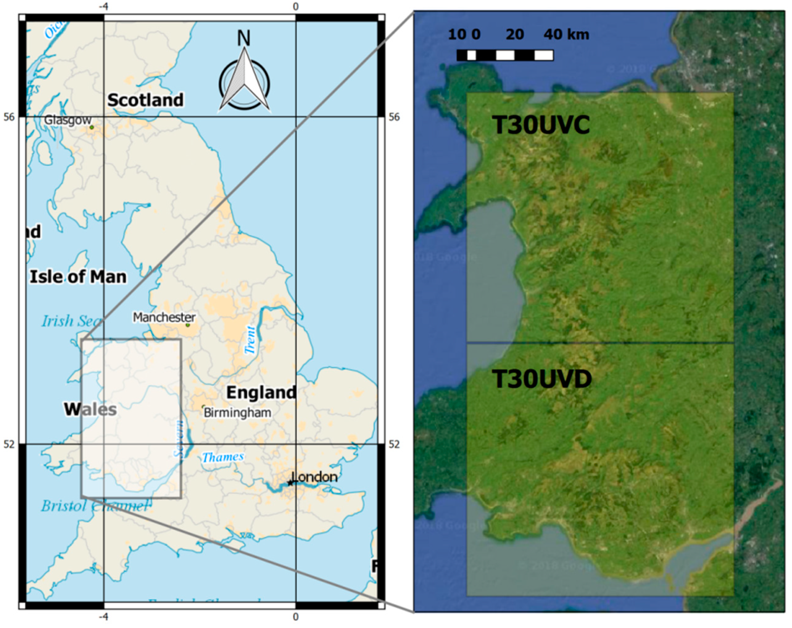
2.1. Study Area
2.2. Datasets
2.2.1. Landsat 8
2.2.2. Indices
2.2.3. Sentinel-2
2.2.4. Sentinel-1
2.2.5. Multi-Sensor
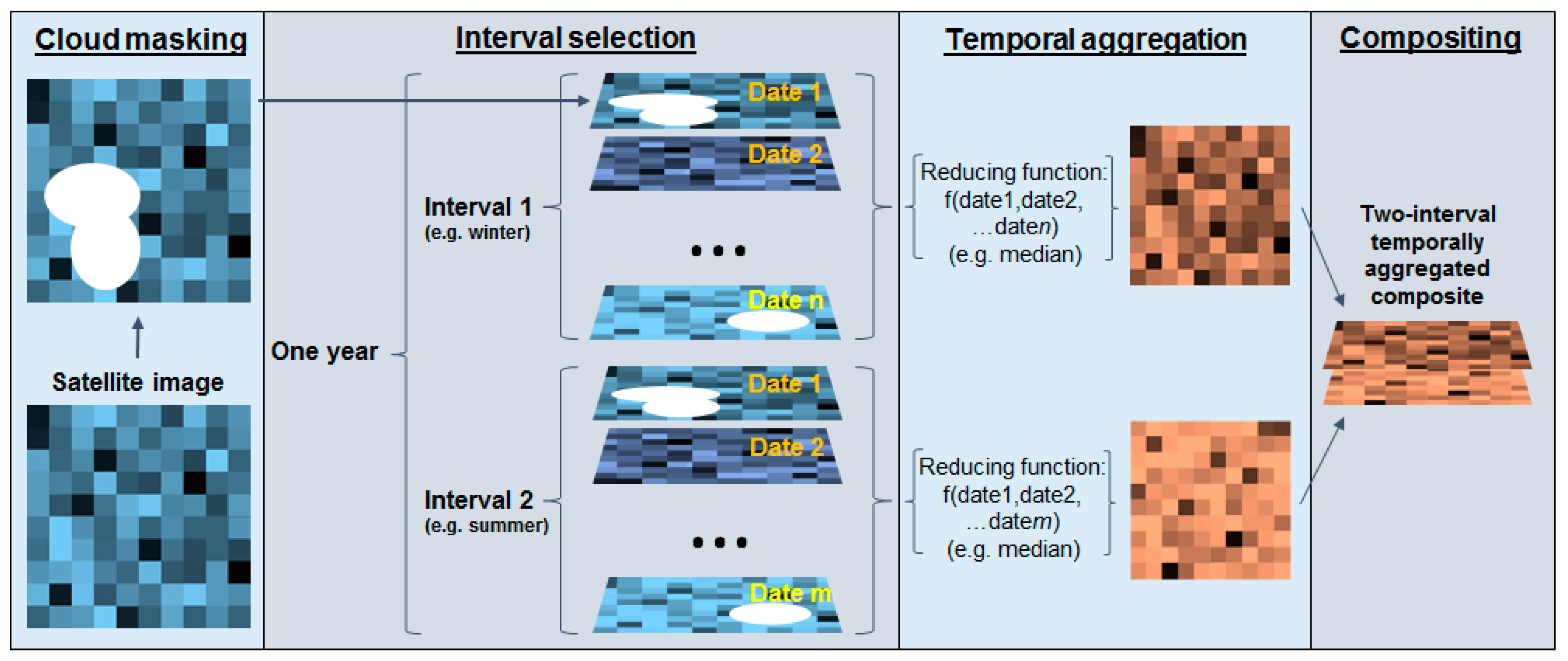
2.2.6. Two-Date Composite
2.3. Land Cover Classification
2.4. Accuracy Assessment
3. Results
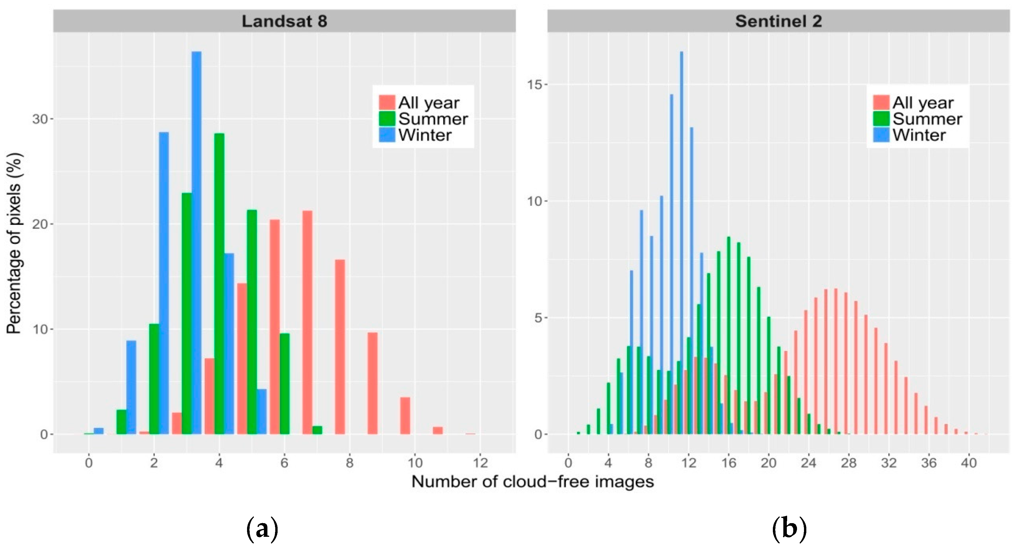
3.1. Cloud Cover
3.2. Classification Accuracy
4. Discussion
5. Conclusions
Supplementary Materials
Author Contributions
Funding
Acknowledgments
Conflicts of Interest
References
- Lambin, E.F.; Geist, H.J.; Lepers, E. Dynamics of land-use and land-cover change in tropical regions. Annu. Rev. Environ. Resour. 2003, 28, 205–241. [Google Scholar] [CrossRef]
- Global Climate Observing System. Essential Climate Variables, 2010. Available online: https://public.wmo.int/en/programmes/global-climate-observing-system/essential-climate-variables (accessed on 1 August 2018).
- Pettorelli, N.; Wegmann, M.; Skidmore, A.; Mucher, S.; Dawson, T.P.; Fernandez, M.; Lucas, R.; Schaepman, M.E.; Wang, T.; O’Connor, B.; et al. Framing the concept of satellite remote sensing essential biodiversity variables: Challenges and future directions. Remote Sens. Ecol. Conserv. 2016, 2, 122–131. [Google Scholar] [CrossRef]
- Lambin, E.F.; Geist, H.J. Land-Use and Land-Cover Change: Local Processes and Global Impacts; Springer Science & Business Media: Berlin, Germany, 2008. [Google Scholar]
- Wulder, M.A.; Coops, N.C.; Roy, D.P.; White, J.C.; Hermosilla, T. Land cover 2.0. Int. J. Remote Sens. 2018, 39, 4254–4284. [Google Scholar] [CrossRef]
- Kovalskyy, V.; Roy, D. The global availability of Landsat 5 tm and Landsat 7 etm+ land surface observations and implications for global 30 m Landsat data product generation. Remote Sens. Environ. 2013, 130, 280–293. [Google Scholar] [CrossRef]
- Li, J.; Roy, D.P. A global analysis of Sentinel-2a, Sentinel-2b and Landsat-8 data revisit intervals and implications for terrestrial monitoring. Remote Sens. 2017, 9, 902. [Google Scholar]
- Gorelick, N.; Hancher, M.; Dixon, M.; Ilyushchenko, S.; Thau, D.; Moore, R. Google earth engine: Planetary-scale geospatial analysis for everyone. Remote Sens. Environ. 2017, 202, 18–27. [Google Scholar] [CrossRef]
- Gevaert, C.M.; García-Haro, F.J. A comparison of STARFM and an unmixing-based algorithm for Landsat and Modis data fusion. Remote Sens. Environ. 2015, 156, 34–44. [Google Scholar] [CrossRef]
- Senf, C.; Leitao, P.J.; Pflugmacher, D.; van der Linden, S.; Hostert, P. Mapping land cover in complex Mediterranean landscapes using Landsat: Improved classification accuracies from integrating multi-seasonal and synthetic imagery. Remote Sens. Environ. 2015, 156, 527–536. [Google Scholar] [CrossRef]
- Zhang, Y.; Atkinson, P.M.; Li, X.; Ling, F.; Wang, Q.; Du, Y. Learning-based spatial–temporal superresolution mapping of forest cover with MODIS images. IEEE Trans. Geosci. Remote Sens. 2017, 55, 600–614. [Google Scholar] [CrossRef]
- Inglada, J.; Vincent, A.; Arias, M.; Tardy, B.; Morin, D.; Rodes, I. Operational high resolution land cover map production at the country scale using satellite image time series. Remote Sens. 2017, 9, 95. [Google Scholar] [CrossRef]
- Griffiths, P.; van der Linden, S.; Kuemmerle, T.; Hostert, P. A pixel-based Landsat compositing algorithm for large area land cover mapping. IEEE J.-STARS 2013, 6, 2088–2101. [Google Scholar] [CrossRef]
- Hermosilla, T.; Wulder, M.A.; White, J.C.; Coops, N.C.; Hobart, G.W. Disturbance-informed annual land cover classification maps of Canada’s forested ecosystems for a 29-year Landsat time series. Can. J. Remote Sens. 2018, 44, 67–87. [Google Scholar] [CrossRef]
- DeFries, R.; Hansen, M.; Townshend, J. Global discrimination of land cover types from metrics derived from AVHRR pathfinder data. Remote Sens. Environ. 1995, 54, 209–222. [Google Scholar] [CrossRef]
- Loveland, T.R.; Reed, B.C.; Brown, J.; Ohlen, D.O.; Zhu, Z.; Yang, L.; Merchant, J.W. Development of a global land cover characteristics database and IGBP DISCover from 1 km AVHRR data. Int. J. Remote Sens. 2000, 21, 1303–1330. [Google Scholar] [CrossRef]
- Gebhardt, S.; Wehrmann, T.; Ruiz, M.A.M.; Maeda, P.; Bishop, J.; Schramm, M.; Kopeinig, R.; Cartus, O.; Kellndorfer, J.; Ressl, R.; et al. Mad-mex: Automatic wall-to-wall land cover monitoring for the mexicanredd-mrv program using all Landsat data. Remote Sens. 2014, 6, 3923–3943. [Google Scholar] [CrossRef]
- Winsvold, S.H.; Kaab, A.; Nuth, C. Regional glacier mapping using optical satellite data time series. IEEE J.-STARS 2016, 9, 3698–3711. [Google Scholar] [CrossRef]
- Verhegghen, A.; Eva, H.; Ceccherini, G.; Achard, F.; Gond, V.; Gourlet-Fleury, S.; Cerutti, P.O. The potential of sentinel satellites for burnt area mapping and monitoring in the Congo basin forests. Remote Sens. 2016, 8, 986. [Google Scholar] [CrossRef]
- Zhu, Z.; Woodcock, C.E. Continuous change detection and classification of land cover using all available Landsat data. Remote Sens. Environ. 2014, 144, 152–171. [Google Scholar] [CrossRef]
- Armitage, R.P.; Ramirez, F.A.; Danson, F.M.; Ogunbadewa, E.Y. Probability of cloud-free observation conditions across Great Britain estimated using MODIS cloud mask. Remote Sens. Lett. 2013, 4, 427–435. [Google Scholar] [CrossRef]
- Blackstock, T.; Burrows, C.; Howe, E.; Stevens, D.; Stevens, J. Habitat inventory at a regional scale: A comparison of estimates of terrestrial broad habitat cover from stratified sample field survey and full census field survey for wales, UK. J. Environ. Manag. 2007, 85, 224–231. [Google Scholar] [CrossRef]
- Gómez, C.; White, J.C.; Wulder, M.A. Optical remotely sensed time series data for land cover classification: A review. ISPRS J. Photogramm. 2016, 116, 55–72. [Google Scholar] [CrossRef]
- Khatami, R.; Mountrakis, G.; Stehman, S.V. A meta-analysis of remote sensing research on supervised pixel-based land-cover image classification processes: General guidelines for practitioners and future research. Remote Sens. Environ. 2016, 177, 89–100. [Google Scholar] [CrossRef]
- Zhu, Z.; Woodcock, C.E. Object-based cloud and cloud shadow detection in Landsat imagery. Remote Sens. Environ. 2012, 118, 83–94. [Google Scholar] [CrossRef]
- Foga, S.; Scaramuzza, P.L.; Guo, S.; Zhu, Z.; Dilley, R.D.; Beckmann, T.; Schmidt, G.L.; Dwyer, J.L.; Hughes, M.J.; Laue, B. Cloud detection algorithm comparison and validation for operational Landsat data products. Remote Sens. Environ. 2017, 194, 379–390. [Google Scholar] [CrossRef]
- Tucker, C.J. Red and photographic infrared linear combinations for monitoring vegetation. Remote Sens. Environ. 1979, 8, 127–150. [Google Scholar] [CrossRef]
- Wilson, E.H.; Sader, S.A. Detection of forest harvest type using multiple dates of Landsat tm imagery. Remote Sens. Environ. 2002, 80, 385–396. [Google Scholar] [CrossRef]
- McFeeters, S.K. The use of the normalized difference water index (NDWI) in the delineation of open water features. Int. J. Remote Sens. 1996, 17, 1425–1432. [Google Scholar] [CrossRef]
- Gatti, A.; Bertolini, A. Sentinel-2 Products Specification Document, 2015. Available online: https://sentinel.esa.int/documents/247904/349490/S2_MSI_Product_Specification.pdf (accessed on 3 August 2018).
- Bourbigot, M.; Piantanida, R. Sentinel-1 User Handbook; European Space Agency (ESA): Paris, France, 2016. [Google Scholar]
- Farr, T.G.; Kobrick, M. Shuttle Radar Topography Mission produced a wealth of data. EOS Trans. Am. Geophys. Union 2000, 81, 583–585. [Google Scholar] [CrossRef]
- Yommy, A.S.; Liu, R.; Wu, S. SAR image despeckling using refined lee filter. In Proceedings of the 2015 7th International Conference on Intelligent HumanMachine Systems and Cybernetics (IHMSC), Hangzhou, China, 26–27 August 2015; Volume 2, pp. 260–265. [Google Scholar]
- Abdikan, S.; Sanli, F.; Ustuner, M.; Caló, F. Land cover mapping using sentinel-1 SAR data. ISPRS Int. Arch. Photogramm. Remote Sens. Spat. Inf. Sci. 2016, XLI-B7, 757–761. [Google Scholar] [CrossRef]
- Louis, J.; Debaecker, V.; Pflug, B.; Main-Knorn, M.; Bieniarz, J.; Mueller-Wilm, U.; Cadau, E.; Gascon, F. Sentinel-2 sen2cor: L2a processor for users. In Proceedings of the Living Planet Symposium, Prague, Czech Republic, 9–13 May 2016; pp. 1–8. [Google Scholar]
- Gao, M.; Gong, H.; Zhao, W.; Chen, B.; Chen, Z.; Shi, M. An improved topographic correction model based on minnaert. GISci. Remote Sens. 2016, 53, 247–264. [Google Scholar] [CrossRef]
- Fuller, R.; Smith, G.; Sanderson, J.; Hill, R.; Thomson, A.; Cox, R.; Brown, N.; Clarke, R.; Rothery, P.; Gerard, F. Countryside Survey 2000 Module 7. Land Cover Map 2000; Final Report; Centre for Ecology & Hydrology: Lancaster, UK, 2002. [Google Scholar]
- Morton, D.; Rowland, C.; Wood, C.; Meek, L.; Marston, C.; Smith, G.; Wadsworth, R.; Simpson, I. Final Report for LCM2007: The New UK Land Cover Map; Centre for Ecology & Hydrology: Lancaster, UK, 2011. [Google Scholar]
- Jackson, D. Guidance on the Interpretation of the Biodiversity Broad Habitat Classification (Terrestrial and Freshwater Types): Definitions and the Relationship with Other Habitat Classifications; Joint Nature Conservation Committee: London, UK, 2000. [Google Scholar]
- Breiman, L. Random forests. Mach. Learn. 2001, 45, 5–32. [Google Scholar] [CrossRef]
- Hall, M.; Frank, E.; Holmes, G.; Pfahringer, B.; Reutemann, P.; Witten, I.H. The Weka data mining software: An update. SIGKDD Explor. 2009, 11, 10–18. [Google Scholar] [CrossRef]
- Emmett, B.; Abdalla, M.; Anthony, S.; Astbury, S.; August, T.; Barrett, G.; Beckmann, B.; Biggs, J.; Botham, M.; Bradley, D.; et al. Glastir Monitoring & Evaluation Programme. Second Year Annual Report; Centre for Ecology & Hydrology: Lancaster, UK, 2015. [Google Scholar]
- UK Forestry Commission. National Forest Inventory Woodland England 2015. 2016. Available online: https://data.gov.uk/dataset/ae33371a-e4da-4178-a1df-350ccfcc6cee/national-forest-inventory-woodland-england-2015 (accessed on 25 October 2018).
- Blackstock, T.; Stevens, J.; Howe, L.; Jones, P. Habitats of Wales: A Comprehensive Field Survey; University of Wales Press: Cardiff, UK, 2010; pp. 1979–1997. [Google Scholar]
- Wan, T.; Jun, H.; Hui Zhang, P.W.; Hua, H. Kappa coefficient: A popular measure of rater agreement. Shanghai Arch. Psychiatry 2015, 27, 62. [Google Scholar]
- Congalton, R.G.; Gu, J.; Yadav, K.; Thenkabail, P.; Ozdogan, M. Global land cover mapping: A review and uncertainty analysis. Remote Sens. 2014, 6, 12070–12093. [Google Scholar] [CrossRef]
- Chen, B.; Huang, B.; Xu, B. Multi-source remotely sensed data fusion for improving land cover classification. ISPRS J. Photogramm. 2017, 124, 27–39. [Google Scholar] [CrossRef]
- Qadri, S.; Khan, D.M.; Qadri, S.F.; Razzaq, A.; Ahmad, N.; Jamil, M.; Nawaz Shah, A.; Shah Muhammad, S.; Saleem, K.; Awan, S.A. Multisource data fusion framework for land use/land cover classification using machine vision. J. Sens. 2017, 2017, 3515418. [Google Scholar] [CrossRef]
- Foody, G.M. The impact of imperfect ground reference data on the accuracy of land cover change estimation. Int. J. Remote Sens. 2009, 30, 3275–3281. [Google Scholar] [CrossRef]
- Fan, X.; Liu, Y. A global study of NDVI difference among moderate-resolution satellite sensors. ISPRS J. Photogramm. 2016, 121, 177–191. [Google Scholar] [CrossRef]
- Feng, D.; Yu, L.; Zhao, Y.; Cheng, Y.; Xu, Y.; Li, C.; Gong, P. A multiple dataset approach for 30-m resolution land cover mapping: A case study of continental Africa. Int. J. Remote Sens. 2018, 39, 3926–3938. [Google Scholar] [CrossRef]
- Bargiel, D. A new method for crop classification combining time series of radar images and crop phenology information. Remote Sens. Environ. 2017, 198, 369–383. [Google Scholar] [CrossRef]
- Haarpaintner, J.; Davids, C.; Storvold, R.; Johansen, K.; Arnason, K.; Rauste, Y.; Mutanen, T. Boreal forest land cover mapping in Iceland and Finland using Sentinel-1A. In Proceedings of the Living Planet Symposium, Prague, Czech Republic, 9–13 May 2016; Volume 740, p. 197. [Google Scholar]
- Coluzzi, R.; Imbrenda, V.; Lanfredi, M.; Simoniello, T. A first assessment of the Sentinel 2 Level 1-C cloud mask product to support informed surface analyses. Remote Sens. Environ. 2018, 217, 426–443. [Google Scholar] [CrossRef]
- Storey, J.; Roy, D.P.; Masek, J.; Gascon, F.; Dwyer, J.; Choate, M. A note on the temporary misregistration of Landsat-8 Operational Land Imager (OLI) and Sentinel-2 Multi Spectral Instrument (MSI) imagery. Remote Sens. Environ. 2016, 186, 121–122. [Google Scholar] [CrossRef]
- Yan, L.; Roy, D.P.; Zhang, H.K.; Li, J.; Huang, H. An automated approach for sub-pixel registration of Landsat-8 of Landsat-8 Operational Land Imager (OLI) and Sentinel-2 Multi Spectral Instrument (MSI) imagery. Remote Sens. 2016, 8, 520. [Google Scholar] [CrossRef]
- Claverie, M.; Ju, J.; Masek, J.; Dungan, J.L.; Vermonte, E.F.; Roger, J.; Skakun, S.V.; Justice, C. The Harmonized Landsat and Sentinel-2 surface reflectance data set. Remote Sens. Environ. 2018, 219, 145–161. [Google Scholar] [CrossRef]
- Solberg, A.H.S.; Jain, A.K.; Taxt, T. Multisource classification of remotely sensed data: Fusion of Landsat TM and SAR images. IEEE Trans. Geosci. Remote Sens. 1994, 32, 768–778. [Google Scholar] [CrossRef]
- Haack, B.; Bechdol, M. Integrating multisensor data and radar texture measures for land cover mapping. Comput. Geosci. 2000, 26, 411–421. [Google Scholar] [CrossRef]
- Dusseux, P.; Corpetti, T.; Hubert-Moy, L.; Corgne, S. Combined use of multi-temporal optical and radar satellite images for grassland monitoring. Remote Sens. 2014, 6, 6163–6182. [Google Scholar] [CrossRef]
- Tatsumi, K.; Yamashiki, Y.; Torres, M.A.C.; Taipe, C.L.R. Crop classification of upland fields using random forest of time-series Landsat 7 etm+ data. Comput. Electron. Agric. 2015, 115, 171–179. [Google Scholar] [CrossRef]
- Yu, L.; Liang, L.; Wang, J.; Zhao, Y.; Cheng, Q.; Hu, L.; Liu, S.; Yu, L.; Wang, X.; Zhu, P.; et al. Meta-discoveries from a synthesis of satellite-based land-cover mapping research. Int. J. Remote Sens. 2014, 35, 4573–4588. [Google Scholar] [CrossRef]
- Gong, P.; Yu, L.; Li, C.; Wang, J.; Liang, L.; Li, X.; Ji, L.; Bai, Y.; Cheng, Y.; Zhu, Z. A new research paradigm for global land cover mapping. Ann. GIS 2016, 22, 87–102. [Google Scholar] [CrossRef]
- Hansen, M.C.; Potapov, R.; Moore, R.; Hancher, M.; Turubanova, S.; Tyukavina, A.; Thau, D.; Stehman, S.V.; Goetz, S.J.; Loveland, T.R.; et al. High-resolution global maps of 21st-century forest cover change. Science 2013, 6160, 850–853. [Google Scholar] [CrossRef] [PubMed]


| Landsat 8 | Sentinel-2 | Sentinel-1 | |
|---|---|---|---|
| Sensor (type) | OLI (optical) | MSI (optical) | C-SAR (radar) |
| Spatial resolution (m) | 15 */30/100 * | 10/20/60 * | 5 ** |
| Number of bands (used) | 11 (7) | 12 (9) | 1 |
| Spectral bands (µm) | 0.435–0.451, 0.452−0.512, 0.533–0.590, 0.636–0.673, 0.851−0.879, 1.566–1.651, 10.60–11.19 *, 11.50–12.51, 2.107–2.294, 0.503–0.676 *, 1.363–1.384 * | 0.449–0.545 *, 0.458–0.523, 0.543–0.578, 0.650−0.680, 0.698–0.713, 0.733−0.748, 0.773–0.793, 0.785−0.899, 0.855−0.875 *, 0.932−0.958 *, 1.338−1.414 *, 1.565−1.655, 2.100−2.280 | |
| Repeat Frequency (days) | 16 | 10 | 12 |
| Swath (km) | 180 | 290 | 80 ** |
| Polarization | Not Applicable | Not Applicable | Dual (HH + HV, VV + VH) ** |
| Type | Name | Sensor | Bands | Metric | Intervals |
|---|---|---|---|---|---|
| Landsat 8 | l8_med2 | L8 | B1-7 | median | 2 |
| l8_mea2 | L8 | B1-7 | mean | 2 | |
| l8_var2 | L8 | B1-7 | median and variance | 2 | |
| l8_med1 | L8 | B1-7 | median | 1 | |
| l8_mea1 | L8 | B1-7 | mean | 1 | |
| l8_var1 | L8 | B1-7 | median and variance | 1 | |
| Indices | ndvi_med2 | L8 | NDVI | median | 2 |
| ndvi_med1 | L8 | NDVI | median | 1 | |
| ndvi_var1 | L8 | NDVI | median and variance | 1 | |
| ndvi_mea1 | L8 | NDVI | mean | 1 | |
| ndmi_var1 | L8 | NDVI/NDMI | median and variance | 1 | |
| ndmi_med2 | L8 | NDVI/NDMI | median | 2 | |
| ndwi_var1 | L8 | NDVI/NDWI | median and variance | 1 | |
| ndwi_med2 | L8 | NDVI/NDWI | median | 2 | |
| Sentinel 2 | s2_med1 | S2 | B2-8,11,12 | median | 1 |
| s2_var1 | S2 | B2-8,11,12 | median and variance | 1 | |
| s2_med2 | S2 | B2-8,11,12 | median | 2 | |
| s2_var2 | S2 | B2-8,11,12 | median and variance | 2 | |
| s2_mea2 | S2 | B2-8,11,12 | mean | 2 | |
| s2_med3 | S2 | B2-8,11,12 | median | 3 | |
| s2_med4 | S2 | B2-8,11,12 | median | 4 | |
| Sentinel 1 | s1_med1 | S1 | VV,VH,(VV-VH) | median | 1 |
| s1_med2 | S1 | VV,VH,(VV-VH) | median | 2 | |
| s1_med3 | S1 | VV,VH,(VV-VH) | median | 3 | |
| s1_med4 | S1 | VV,VH,(VV-VH) | median | 4 | |
| s1_med6 | S1 | VV,VH,(VV-VH) | median | 6 | |
| s1_med12 | S1 | VV,VH,(VV-VH) | median | 12 | |
| Combined | s1_s2 | S1; S2 | VV,VH,(VV-VH); B2-8,11,12 | median | 12; 2 |
| s2_l8 | S2; L8 | B2-8,11,12; B1-7 | median | 2; 2 | |
| s1_s2_l8 | S1; S2; L8 | VV,VH,(VV-VH); B2-8,11,12; B1-7 | median | 12; 2; 2 | |
| Two-date | traditional | S2 | B2-8,11,12 | reflectance | 2 |
| composite | auto_cm1 | S2 | B2-8,11,12 | reflectance | 2 |
| Land Cover Class | Description | Validation Data Classes * |
|---|---|---|
| Broadleaf woodland | Broadleaved tree species and mixed | “Broadleaved, Mixed |
| woodland | and Yew Woodland” | |
| Coniferous woodland | Coniferous tree species where they exceed 80% of the total cover | “Coniferous Woodland” |
| Arable | Arable, horticultural and ploughed land; annual leys, rotational set-aside and fallow | “Arable and Horticulture” |
| Grassland | Managed grasslands and other semi-natural | “Improved Grassland” |
| grasslands (grasses and herbs) on | “Calcareous Grassland” | |
| non acidic soils | “Neutral Grassland” | |
| Acid grassland | Grasses and herbs on soils derived from acidic bedrock | “Acid Grassland” |
| Bog and fen | Wetlands with peat-forming vegetation | “Bog” |
| such as bog, fen, fen meadows, rush pasture, swamp, flushes and springs | “Fen, Marsh and Swamp” | |
| Heather | Vegetation that has more than a 25% cover of species from the heath family | “Dwarf Shrub Heath” |
| Inland rock | Natural and artificial exposed rock surfaces | “Inland Rock” |
| Saltwater | Sea waters | “Saltwater” |
| Freshwater | Lakes, pools, rivers and man-made waters | “Freshwater” |
| Coastal | Beaches, sand dunes, ledges, pools | “Supralittoral Rock” |
| and exposed rock in the maritime zone | “Supralittoral Sediment” “Littoral Rock” “Littoral Sediment” | |
| Saltmarsh | Vegetated portions of intertidal mudflats; species adapted to immersion by tides | “Littoral Sediment” ** |
| Built-up areas | Urban and rural settlements | “Built-up Areas and Gardens” |
© 2019 by the authors. Licensee MDPI, Basel, Switzerland. This article is an open access article distributed under the terms and conditions of the Creative Commons Attribution (CC BY) license (http://creativecommons.org/licenses/by/4.0/).
Share and Cite
Carrasco, L.; O’Neil, A.W.; Morton, R.D.; Rowland, C.S. Evaluating Combinations of Temporally Aggregated Sentinel-1, Sentinel-2 and Landsat 8 for Land Cover Mapping with Google Earth Engine. Remote Sens. 2019, 11, 288. https://doi.org/10.3390/rs11030288
Carrasco L, O’Neil AW, Morton RD, Rowland CS. Evaluating Combinations of Temporally Aggregated Sentinel-1, Sentinel-2 and Landsat 8 for Land Cover Mapping with Google Earth Engine. Remote Sensing. 2019; 11(3):288. https://doi.org/10.3390/rs11030288
Chicago/Turabian StyleCarrasco, Luis, Aneurin W. O’Neil, R. Daniel Morton, and Clare S. Rowland. 2019. "Evaluating Combinations of Temporally Aggregated Sentinel-1, Sentinel-2 and Landsat 8 for Land Cover Mapping with Google Earth Engine" Remote Sensing 11, no. 3: 288. https://doi.org/10.3390/rs11030288
APA StyleCarrasco, L., O’Neil, A. W., Morton, R. D., & Rowland, C. S. (2019). Evaluating Combinations of Temporally Aggregated Sentinel-1, Sentinel-2 and Landsat 8 for Land Cover Mapping with Google Earth Engine. Remote Sensing, 11(3), 288. https://doi.org/10.3390/rs11030288