Evaluation of Bias Correction Methods for GOSAT SWIR XH2O Using TCCON data

 , , ,
, , ,  , , ,
, , ,
Abstract
:
1. Introduction
2. Data and Methods
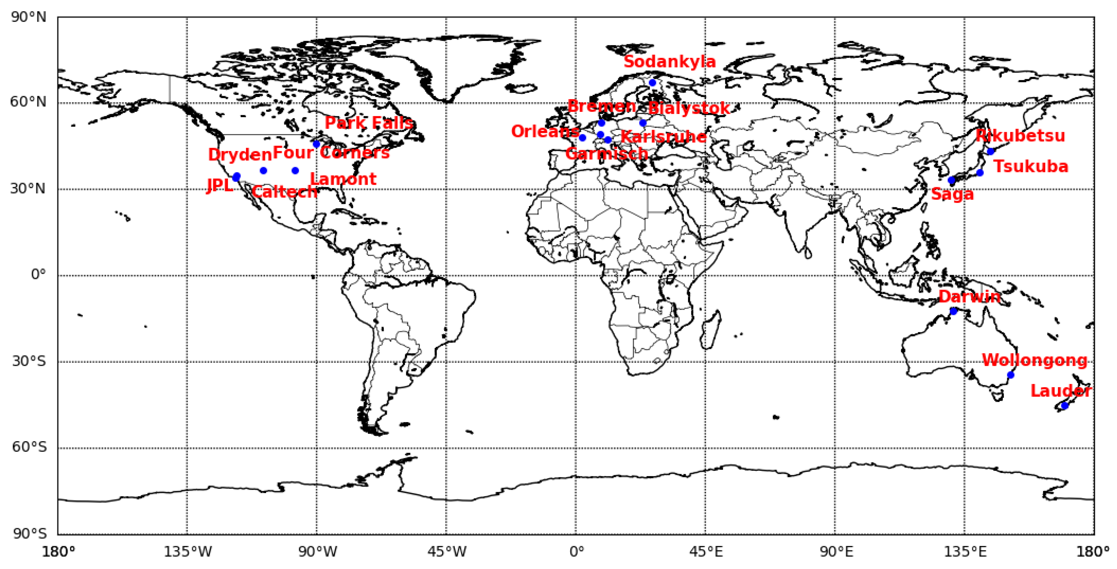
2.1. Data
2.2. Methods
2.2.1. Empirically Derived Bias Correction
2.2.2. Altitude Bias Correction
2.2.3. Combined Method
3. Results
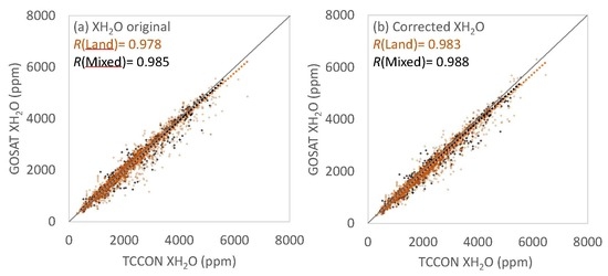
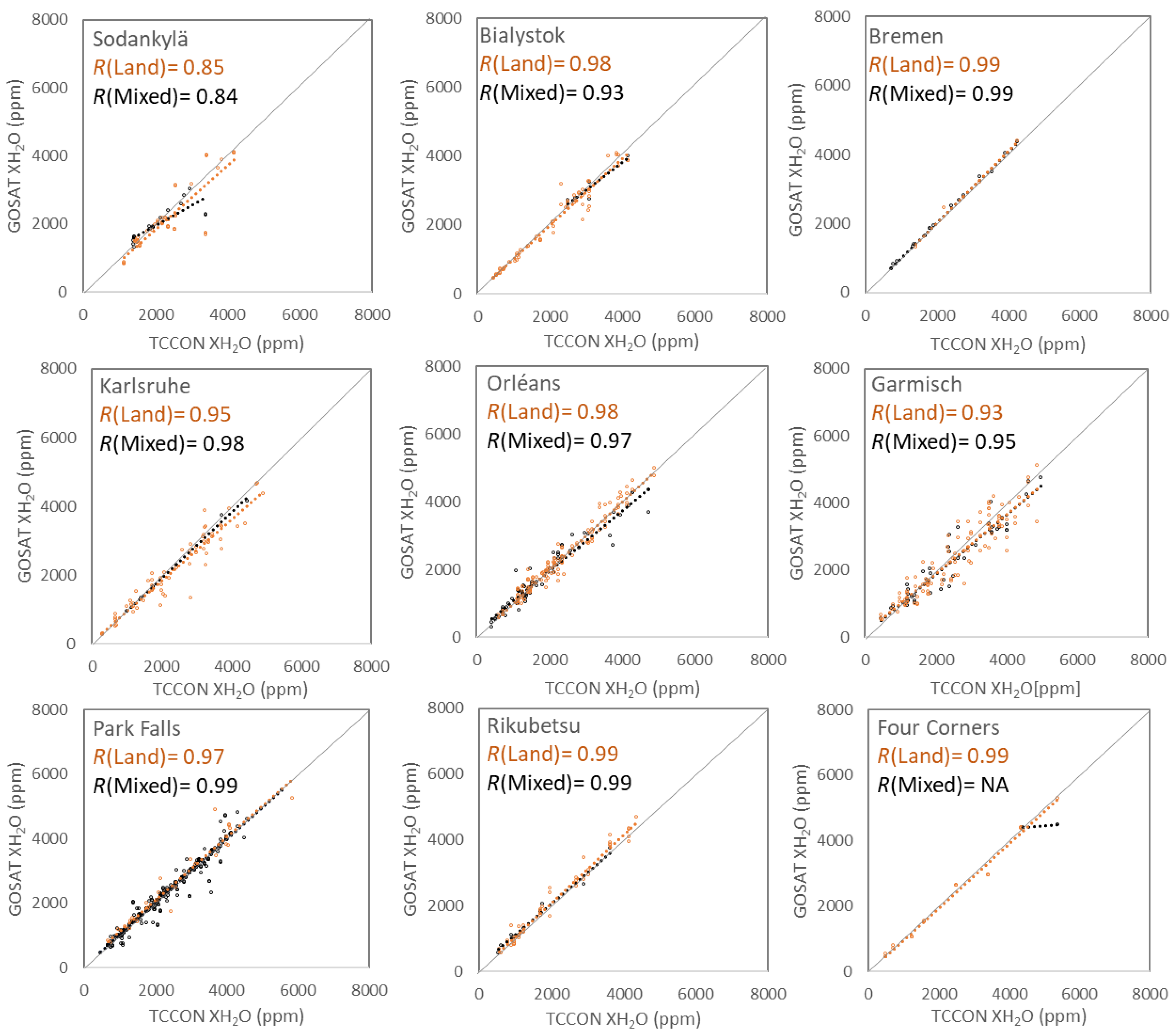
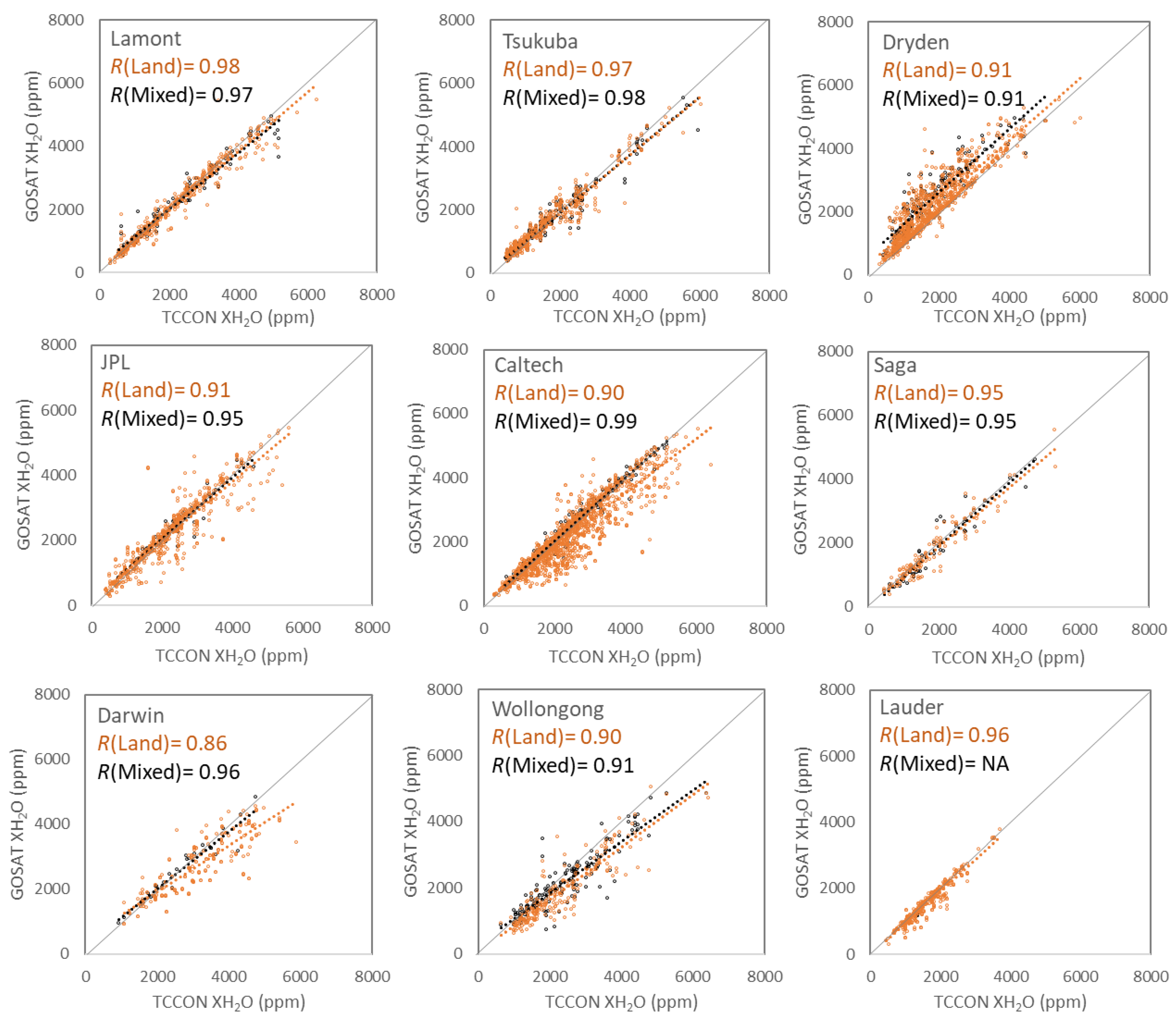
3.1. Comparison between the GOSAT SWIR XH2O and TCCON XH2O
3.2. Bias Correction
4. Discussion
5. Conclusions
Author Contributions
Funding
Acknowledgments
Conflicts of Interest
Appendix A

| TCCON Sites (Lat (°), Lon (°), Alt. (m)) | Radiosonde Sites (Lat (°), Lon (°), Alt. (m)) | Differences between the TCCON and Radiosonde Sites | |
|---|---|---|---|
| Horizontal Distances (km) | ΔAlt. (m) | ||
| Sodankylä (67.37, 26.63, 188) | Sodankylä (67.37, 26.65, 178) | 0.9 | 10 |
| Białystok (53.23, 23.03, 180) | Legionowo (52.40, 20.97, 96) | 166.6 | 84 |
| Bremen (53.10, 8.85, 30) | Bergen (52.82, 9.93, 70) | 78.8 | −40 |
| Karlsruhe (49.10, 8.44, 116) | Stuttgart (48.83, 9.20, 315) | 63.2 | −199 |
| Orléans (47.97, 2.11, 130) | Trappes (48.77, 2.00, 168) | 89.4 | −38 |
| Garmisch (47.48, 11.06, 740) | Altenstadt (47.83, 10.87, 738) | 41.5 | 2 |
| Park Falls (45.94, −90.27, 440) | Green Bay (44.48, −88.13, 214) | 233.6 | 226 |
| Four Corners (36.80, −108.48, 1643) | Grand Junction (39.12, −108.52, 1474) | 258.3 | 169 |
| Lamont (36.60, −97.49, 320) | Lamont (36.62, −97.48, 315) | 2.4 | 5 |
| Tsukuba (36.05, 140.12, 30) | Tateno (36.05, 140.13, 31) | 0.9 | −1 |
| JPL (34.20, −118.18, 390) | Vandenberg AFB (34.75, −120.57, 100) | 227.7 | 290 |
| Saga (33.24, 130.29, 8) | Fukuoka (33.58, 130.38, 15) | 38.8 | −7 |
| Darwin (−12.43, 130.89, 30) | Darwin (−12.43, 130.87, 29) | 2.2 | 1 |
| Wollongong (−34.41, 150.88, 30) | Williamtown (−32.82, 151.83, 9) | 197.7 | 21 |
| Lauder (−45.05, 169.68, 370) | Invercargill (−46.42, 168.32, 4) | 185.5 | 366 |
| Rikubetsu (43.46, 143.77, 361) | Kushiro (42.95, 144.44, 14) | 78.6 | 347 |
| Dryden (34.96, −117.88, 700) | Edwards AFB (34.92, −117.90, 705) | 4.8 | −5 |
| TCCONSites | Jan | Feb | Mar | Apr | May | Jun | Jul | Aug | Sep | Oct | Nov | Dec |
|---|---|---|---|---|---|---|---|---|---|---|---|---|
| Sodankylä | 3.8 | 3.9 | 4.3 | 4.1 | 3.9 | 3.7 | 3.8 | 4.0 | 4.2 | 4.0 | 4.0 | 4.1 |
| Bialystok | 3.7 | 3.9 | 4.1 | 4.0 | 3.8 | 3.8 | 3.7 | 3.8 | 4.0 | 4.1 | 3.9 | 3.9 |
| Bremen | 4.1 | 4.1 | 4.5 | 4.1 | 3.9 | 4 | 3.8 | 3.9 | 4.1 | 4.1 | 4.2 | 4.1 |
| Karlsruhe | 4.1 | 4.1 | 4.3 | 4.1 | 4.0 | 3.9 | 3.8 | 3.9 | 4.1 | 4.0 | 4.0 | 3.9 |
| Orléans | 4.3 | 4.3 | 4.5 | 4.2 | 4.1 | 4.0 | 3.9 | 3.9 | 4.1 | 4.1 | 4.2 | 4.2 |
| Garmisch | 4.1 | 4.1 | 4.5 | 4.3 | 4.1 | 4.0 | 4.0 | 4.0 | 4.3 | 4.2 | 4.2 | 4.0 |
| ParkFalls | 3.3 | 3.6 | 3.6 | 3.3 | 3.7 | 3.8 | 3.9 | 4.1 | 4.1 | 3.7 | 3.7 | 3.6 |
| Rikubetsu | 4.6 | 4.5 | 4.0 | 3.8 | 3.5 | 3.5 | 3.4 | 3.4 | 3.7 | 4.0 | 4.3 | 4.2 |
| FourCorners | 3.7 | 4.2 | 3.9 | 3.7 | 3.5 | 3.2 | 3.2 | 3.4 | 3.5 | 3.7 | 4.0 | 3.8 |
| Lamont | 3.6 | 4.0 | 4.1 | 4.1 | 4.3 | 4.1 | 3.6 | 3.7 | 3.6 | 3.8 | 4.1 | 3.7 |
| Tsukuba | 4.2 | 3.6 | 3.6 | 4.0 | 3.9 | 3.6 | 3.5 | 3.6 | 3.6 | 3.6 | 4.0 | 3.9 |
| Dryden | 3.5 | 4.5 | 4.8 | 4.4 | 4.3 | 4.1 | 3.4 | 3.6 | 3.5 | 4.1 | 4.4 | 4.2 |
| JPL | 3.9 | 4.5 | 4.5 | 4.5 | 4.4 | 4.2 | 3.7 | 4.0 | 4.0 | 4.4 | 4.5 | 4.2 |
| Saga | 4.2 | 3.6 | 3.6 | 3.8 | 3.7 | 3.5 | 3.5 | 3.4 | 3.6 | 3.9 | 3.9 | 4.1 |
| Darwin | 3.6 | 3.7 | 3.7 | 3.9 | 3.8 | 4.1 | 4.0 | 4.8 | 4.6 | 4.2 | 4.0 | 3.7 |
| Wollongong | 4.1 | 4.0 | 4.3 | 4.4 | 4.5 | 4.5 | 4.5 | 4.7 | 4.7 | 4.4 | 4.3 | 4.0 |
| Lauder | 3.9 | 3.9 | 3.9 | 4.0 | 4.2 | 4.4 | 4.5 | 4.6 | 4.3 | 4.2 | 3.9 | 3.9 |
References
- Starr, D.O.; Melfi, S.H. The Role of Water Vapor in Climate—A Strategic Research Plan for the Proposed GEWEX Water Vapor Project (GVaP). In Proceedings of the NASA Conference Publication 3120, Tidewater Inn, Easton, MD, USA, 30 October–1 November 1990. [Google Scholar]
- Jacob, D. The role of water vapor in the atmosphere. A short overview from a climate modeller’s point of view. Phys. Chem. Earth Part A Solid Earth Geod. 2001, 26, 523–527. [Google Scholar] [CrossRef]
- Thies, B.; Bendix, J. Review Satellite based remote sensing of weather and climate: Recent achievements and future perspectives. Meteorol. Appl. 2011, 18, 262–295. [Google Scholar] [CrossRef]
- Water Vapor in the Climate System; AGU Special Report; The American Geophysical Union: Washington, DC, USA, 2009; ISBN 0-87590-865-9.
- Alexander, L.; William, B.; Luca, B.; Claire, E.B.; Jörg, B.; Xavier, C.; Reik, V.D.; Darren, G.; Alexander, G.; Thomas, K.; et al. Validation practices for satellite-based Earth observation data across communities. Rev. Geophys. 2017, 55, 779–817. [Google Scholar] [CrossRef]
- Chazette, P.; Marnas, F.; Totems, J.; Shang, X. Comparison of IASI water vapor retrieval with H2O-Raman lidar in the framework of the Mediterranean HyMeX and ChArMEx programs. Atmos. Chem. Phys. 2014, 14, 9583–9596. [Google Scholar] [CrossRef]
- Ohyama, H.; Kawakami, S.; Shiomi, K.; Morino, I.; Uchino, O. Intercomparison of XH2O Data from the GOSAT TANSO-FTS (TIR and SWIR) and Ground-Based FTS Measurements: Impact of the Spatial Variability of XH2O on the Intercomparison. Remote Sens. 2017, 9, 64. [Google Scholar] [CrossRef]
- Schneider, A.; Borsdorff, T.; Brugh, J.; Hu, H.; Landgraf, J. A full-mission dataset of H2O and HDO columns from SCIAMACHY 2.3 µm reflectance. Atmos. Meas. Tech. 2018, 11, 3339–3350. [Google Scholar] [CrossRef]
- John, V.O.; Holl, G.; Allan, R.P.; Buehler, S.A.; Parker, D.E.; Soden, B.J. Clear-sky biases in satellite infrared estimates of upper tropospheric humidity and its trends. J. Geophys. Res. 2011, 116, D14108. [Google Scholar] [CrossRef]
- John, R.L.; Gregory, E.G. The “Clear-Sky Bias” of TOVS Upper-Tropospheric Humidity. J. Clim. 2000, 13, 4034–4041. [Google Scholar] [CrossRef]
- Hegglin, M.I.; Plummer, D.A.; Shepherd, T.G.; Scinocca, J.F.; Anderson, J.; Froidevaux, L.; Funke, B.; Hurst, D.; Rozanov, A.; Urban, J.; et al. Vertical structure of stratospheric water vapour trends derived from merged satellite data. Nat. Geosci. 2014, 7, 768–776. [Google Scholar] [CrossRef]
- Kuze, A.; Suto, H.; Nakajima, M.; Hamazaki, T. Thermal and near infrared sensor for carbon observation Fourier-transform spectrometer on the Greenhouse Gases Observing Satellite for greenhouse gases monitoring. Appl. Opt. 2009, 48, 6716–6733. [Google Scholar] [CrossRef]
- Wunch, D.; Toon, G.C.; Blavier, J.-F.L.; Washenfelder, R.A.; Notholt, J.; Connor, B.J.; Griffith, D.W.T.; Sherlock, V.; Wennberg, P.O. The total carbon column observing network. Philos. Trans. R. Soc. A 2011, 369, 2087–2112. [Google Scholar] [CrossRef] [PubMed]
- Dunya, A.; Alain, S.; Philippe, K.; Olivier, B.; Stefan, N.; Slimane, B.; Abdenour, I.; Mustapha, M.; Chantal, C. Comparison of total water vapour content in the Arctic derived from GNSS, AIRS, MODIS and SCIAMACHY. Atmos. Meas. Tech. 2018, 11, 2949–2965. [Google Scholar] [CrossRef]
- Buehler, S.A.; Östman, S.; Melsheimer, C.; Holl, G.; Eliasson, S.; John, V.O.; Blumenstock, T.; Hase, F.; Elgered, G.; Raffalski, U.; et al. A multi-instrument comparison of integrated water vapour measurements at a high latitude site. Atmos. Chem. Phys. 2012, 12, 10925–10943. [Google Scholar] [CrossRef]
- Pałm, M.; Melsheimer, C.; Noel, S.; Heise, S.; Notholt, J.; Burrows, J.; Schrems, O. Integrated water vapor above Ny Ålesund, Spitsbergen: A multi-sensor intercomparison. Atmos. Chem. Phys. 2010, 10, 1215–1226. [Google Scholar] [CrossRef]
- Niell, A.E.; Coster, A.J.; Solheim, F.S.; Mendes, V.B.; Toor, P.C.; Langley, R.B.; Upham, C.A. Comparison of measurements of atmospheric wet delay by radiosonde, water vapor radiometer, GPS, and VLBI. J. Atmos. Ocean. Technol. 2001, 80, 830–850. [Google Scholar] [CrossRef]
- Sussmann, R.; Borsdorff, T.; Rettinger, M.; Camy-Peyret, C.; Demoulin, P.; Duchatelet, P.; Mahieu, E.; Servais, C. Harmonized retrieval of column-integrated atmospheric water vapor from the FTIR network—First examples for long-term records and station trends. Atmos. Chem. Phys. 2009, 9, 8987–8999. [Google Scholar] [CrossRef]
- Vogelmann, H.; Sussmann, R.; Trickl, T.; Borsdorff, T. Intercomparison of atmospheric water vapor soundings from the differential absorption lidar (DIAL) and the solar FTIR system on Mt. Zugspitze. Atmos. Meas. Tech. 2011, 4, 835–841. [Google Scholar] [CrossRef]
- Vogelmann, H.; Sussmann, R.; Trickl, T.; Reichert, A. Spatiotemporal variability of water vapor investigated using lidar and FTIR vertical soundings above the Zugspitze. Atmos. Chem. Phys. 2015, 15, 3135–3148. [Google Scholar] [CrossRef]
- Sapucci, L.F.; Machado, L.A.T.; Monico, J.F.G.; Plana Fattori, A. Intercomparison of integrated water vapor estimates from multisensors in the amazonian region. J. Atmos. Ocean. Technol. 2007, 24, 1880–1894. [Google Scholar] [CrossRef]
- Van Malderen, R.; Brenot, H.; Pottiaux, E.; Beirle, S.; Hermans, C.; De Mazière, M.; Wagner, T.; De Backer, H.; Bruyninx, C. A multi-site intercomparison of integrated water vapour observations for climate change analysis. Atmos. Meas. Tech. 2014, 7, 2487–2512. [Google Scholar] [CrossRef]
- Bedka, S.; Knuteson, R.; Revercomb, H.; Tobin, D.; Turner, D. An assessment of the absolute accuracy of the Atmospheric Infrared Sounder v5 precipitable water vapor product at tropical, midlatitude, and arctic ground-truth sites: September 2002 through August 2008. J. Geophys. Res. 2010, 115, D17310. [Google Scholar] [CrossRef]
- Weaver, D.; Strong, K.; Walker, K.A.; Sioris, C.; Schneider, M.; McElroy, C.T.; Vömel, H.; Sommer, M.; Weigel, K.; Rozanov, A.; et al. Comparison of ground-based and satellite measurements of water vapour vertical profiles over Ellesmere Island, Nunavut. Atmos. Meas. Tech. Discuss. 2018. [Google Scholar] [CrossRef]
- Morino, I.; Uchino, O.; Inoue, M.; Yoshida, Y.; Yokota, T.; Wennberg, P.O.; Toon, G.C.; Wunch, D.; Roehl, C.M.; Notholt, J.; et al. Preliminary validation of column-averaged volume mixing ratios of carbon dioxide and methane retrieved from GOSAT short-wavelength infrared spectra. Atmos. Meas. Tech. 2011, 4, 1061–1076. [Google Scholar] [CrossRef]
- Wunch, D.; Wennberg, P.O.; Toon, G.C.; Connor, B.J.; Fisher, B.; Osterman, G.B.; Frankenberg, C.; Mandrake, L.; O’Dell, C.; Ahonen, P.; et al. A method for evaluating bias in global measurements of CO2 total columns from space. Atmos. Chem. Phys. 2011, 11, 12317–12337. [Google Scholar] [CrossRef]
- Inoue, M.; Morino, I.; Uchino, O.; Miyamoto, Y.; Saeki, T.; Yoshida, Y.; Yokota, T.; Sweeney, C.; Tans, P.P.; Biraud, S.C.; et al. Validation of XCH4 derived from SWIR spectra of GOSAT TANSO-FTS with aircraft measurement data. Atmos. Meas. Tech. 2014, 7, 2987–3005. [Google Scholar] [CrossRef]
- Iwasaki, C.; Imasu, R.; Bril, A.; Yokota, T.; Yoshida, Y.; Morino, I.; Oshchepkov, S.; Rokotyan, N.; Zakharov, V.; Gribanov, K. Validation of GOSAT SWIR XCO2 and XCH4 Retrieved by PPDF-S Method and Comparison with Full Physics Method. SOLA 2017, 13, 168–173. [Google Scholar] [CrossRef]
- Yoshida, Y.; Kikuchi, N.; Morino, I.; Uchino, O.; Oshchepkov, S.; Bril, A.; Saeki, T.; Schutgens, N.; Toon, G.C.; Wunch, D.; et al. Improvement of the retrieval algorithm for GOSAT SWIR XCO2 and XCH4 and their validation using TCCON data. Atmos. Meas. Tech. 2013, 6, 1533–1547. [Google Scholar] [CrossRef]
- Ohyama, H.; Kawakami, S.; Tanaka, T.; Morino, I.; Uchino, O.; Inoue, M.; Sakai, T.; Nagai, T.; Yamazaki, A.; Uchiyama, A.; et al. Observations of XCO2 and XCH4 with ground-based high-resolution FTS at Saga, Japan, and comparisons with GOSAT products. Atmos. Meas. Tech. 2015, 8, 5263–5276. [Google Scholar] [CrossRef]
- Dupuy, E.; Morino, I.; Deutscher, N.M.; Yoshida, Y.; Uchino, O.; Connor, B.J.; DeMazière, M.; Griffith, D.W.T.; Hase, F.; Heikkinen, P.; et al. Comparison of XH2O retrieved from GOSAT short-wavelength infrared spectra with observations from the TCCON network. Remote Sens. 2016, 8, 414. [Google Scholar] [CrossRef]
- Trent, T.; Boesch, H.; Somkuti, P.; Scott, N.A. Observing Water Vapour in the Planetary Boundary Layer from the Short-Wave Infrared. Remote Sens. 2018, 10, 1469. [Google Scholar] [CrossRef]
- The GOSAT Data Archive Service. Available online: http://data2.gosat.nies.go.jp/ (accessed on 29 January 2019).
- Suto, H.; Yoshida, J.; Desbiens, R.; Kawashima, T.; Kuze, A. Characterization and correction of spectral distortions induced by microvi-brations onboard the GOSAT Fourier transform spectrometer. Appl. Opt. 2013. [Google Scholar] [CrossRef] [PubMed]
- Velazco, V.A.; Deutscher, N.M.; Morino, I.; Uchino, O.; Bukosa, B.; Ajiro, M.; Kamei, A.; Jones, N.B.; Paton-Walsh, C.; Griffith, D.W.T. Satellite and Ground-based Measurements of XCO2 in a Remote Semi-Arid Region of Australia. Earth Syst. Sci. Data Discuss. 2019. [Google Scholar] [CrossRef]
- The TCCON Data Archive. Available online: http://tccondata.org/ (accessed on 29 January 2019).
- Kivi, R.; Heikkinen, P.; Kyrö, E. TCCON Data from Sodankylä, Finland, Release GGG2014R0; TCCON Data Archive, Hosted by CaltechDATA; California Institute of Technology: Pasadena, CA, USA, 2017. [Google Scholar] [CrossRef]
- Deutscher, N.; Notholt, J.; Messerschmidt, J.; Weinzierl, C.; Warneke, T.; Petri, C.; Grupe, P.; Katrynski, K. TCCON Data from Bialystok, Poland, Release GGG2014R0; TCCON Data Archive, Hosted by CaltechDATA; California Institute of Technology: Pasadena, CA, USA, 2017. [Google Scholar] [CrossRef]
- Notholt, J.; Petri, C.; Warneke, T.; Deutscher, N.; Buschmann, M.; Weinzierl, C.; Macatangay, R.; Grupe, P. TCCON Data from Bremen, Germany, Release GGG2014R0; TCCON Data Archive, Hosted by CaltechDATA; California Institute of Technology: Pasadena, CA, USA, 2017. [Google Scholar] [CrossRef]
- Hase, F.; Blumenstock, T.; Dohe, S.; Groß, J.; Kiel, M. TCCON Data from Karlsruhe, Germany, Release GGG2014R0; TCCON Data Archive, Hosted by CaltechDATA; California Institute of Technology: Pasadena, CA, USA, 2017. [Google Scholar] [CrossRef]
- Warneke, T.; Messerschmidt, J.; Notholt, J.; Weinzierl, C.; Deutscher, N.; Petri, C.; Grupe, P.; Vuillemin, C.; Truong, F.; Schmidt, M.; et al. TCCON Data from Orléans, France, Release GGG2014R0; TCCON Data Archive, Hosted by CaltechDATA; California Institute of Technology: Pasadena, CA, USA, 2017. [Google Scholar] [CrossRef]
- Sussmann, R.; Rettinger, M. TCCON Data from Garmisch, Germany, Release GGG2014R0; TCCON Data Archive, Hosted by CaltechDATA; California Institute of Technology: Pasadena, CA, USA, 2017. [Google Scholar] [CrossRef]
- Wennberg, P.O.; Roehl, C.; Wunch, D.; Toon, G.C.; Blavier, J.-F.; Washenfelder, R.; Keppel-Aleks, G.; Allen, N.; Ayers, J. TCCON Data from Park Falls, Wisconsin, USA, Release GGG2014R0; TCCON Data Archive, Hosted by CaltechDATA; California Institute of Technology: Pasadena, CA, USA, 2017. [Google Scholar] [CrossRef]
- Morino, I.; Yokozeki, N.; Matzuzaki, T.; Shishime, A. TCCON Data from Rikubetsu, Hokkaido, Japan, Release GGG2014R2; TCCON Data Archive, Hosted by CaltechDATA; California Institute of Technology: Pasadena, CA, USA, 2017. [Google Scholar] [CrossRef]
- Dubey, M.; Lindenmaier, R.; Henderson, B.; Green, D.; Allen, N.; Roehl, C.; Blavier, J.-F.; Butterfield, Z.; Love, S.; Hamelmann, J.; et al. TCCON Data from Four Corners, NM, USA, Release GGG2014R0; TCCON Data Archive, Hosted by CaltechDATA; California Institute of Technology: Pasadena, CA, USA, 2017. [Google Scholar] [CrossRef]
- Wennberg, P.O.; Wunch, D.; Roehl, C.; Blavier, J.-F.; Toon, G.C.; Allen, N.; Dowell, P.; Teske, K.; Martin, C.; Martin, J. TCCON Data from Lamont, Oklahoma, USA, Release GGG2014R0; TCCON Data Archive, Hosted by CaltechDATA; California Institute of Technology: Pasadena, CA, USA, 2017. [Google Scholar] [CrossRef]
- Morino, I.; Matsuzaki, T.; Ikegami, H.; Shishime, A. TCCON Data from Tsukuba, Ibaraki, Japan, 125HR, Release GGG2014R0; TCCON Data Archive, Hosted by CaltechDATA; California Institute of Technology: Pasadena, CA, USA, 2017. [Google Scholar] [CrossRef]
- Iraci, L.; Podolske, J.; Hillyard, P.; Roehl, C.; Wennberg, P.O.; Blavier, J.-F.; Landeros, J.; Allen, N.; Wunch, D.; Zavaleta, J.; et al. TCCON Data from Armstrong Flight Research Center, Edwards, CA, USA, Release GGG2014R1; TCCON Data Archive, Hosted by CaltechDATA; California Institute of Technology: Pasadena, CA, USA, 2017. [Google Scholar] [CrossRef]
- Wennberg, P.O.; Roehl, C.; Blavier, J.-F.; Wunch, D.; Landeros, J.; Allen, N. TCCON Data from Jet Propulsion Laboratory, Pasadena, California, USA, Release GGG2014R0; TCCON Data Archive, Hosted by CaltechDATA; California Institute of Technology: Pasadena, CA, USA, 2017. [Google Scholar] [CrossRef]
- Wennberg, P.O.; Wunch, D.; Roehl, C.; Blavier, J.-F.; Toon, G.C.; Allen, N. TCCON Data from California Institute of Technology, Pasadena, California, USA, Release GGG2014R1; TCCON Data Archive, Hosted by CaltechDATA; California Institute of Technology: Pasadena, CA, USA, 2017. [Google Scholar] [CrossRef]
- Kawakami, S.; Ohyama, H.; Arai, K.; Okumura, H.; Taura, C.; Fukamachi, T.; Sakashita, M. TCCON Data from Saga, Japan, Release GGG2014R0; TCCON Data Archive, Hosted by CaltechDATA; California Institute of Technology: Pasadena, CA, USA, 2017. [Google Scholar] [CrossRef]
- Griffith, D.W.T.; Deutscher, N.; Velazco, V.A.; Wennberg, P.O.; Yavin, Y.; Keppel Aleks, G.; Washenfelder, R.; Toon, G.C.; Blavier, J.-F.; Murphy, C.; et al. TCCON Data from Darwin, Australia, Release GGG2014R0; TCCON Data Archive, Hosted by CaltechDATA; California Institute of Technology: Pasadena, CA, USA, 2017. [Google Scholar] [CrossRef]
- Griffith, D.W.T.; Velazco, V.A.; Deutscher, N.; Murphy, C.; Jones, N.; Wilson, S.; Macatangay, R.; Kettlewell, G.; Buchholz, R.R.; Riggenbach, M. TCCON Data from Wollongong, Australia, Release GGG2014R0; TCCON Data Archive, Hosted by CaltechDATA; California Institute of Technology: Pasadena, CA, USA, 2017. [Google Scholar] [CrossRef]
- Sherlock, V.; Connor, B.; Robinson, J.; Shiona, H.; Smale, D.; Pollard, D. TCCON Data from Lauder, NewZealand, 120HR, ReleaseGGG2014R0; TCCON Data Archive, Hosted by CaltechDATA; California Institute of Technology: Pasadena, CA, USA, 2017. [Google Scholar] [CrossRef]
- Sherlock, V.; Connor, B.; Robinson, J.; Shiona, H.; Smale, D.; Pollard, D. TCCON Data from Lauder, NewZealand, 125HR, Release GGG2014R0; TCCON Data Archive, Hosted by CaltechDATA; California Institute of Technology: Pasadena, CA, USA, 2017. [Google Scholar] [CrossRef]
- The National Centers for Environmental Prediction reanalysis data. Available online: https://www.ncdc.noaa.gov/data-access/model-data/model-datasets/reanalysis-1-reanalysis-2 (accessed on 29 January 2019).
- Nguyen, H.; Osterman, G.; Wunch, D.; O’Dell, C.; Mandrake, L.; Wennberg, P.; Fisher, B.; Castano, R. A method for colocating satellite XCO2 data to ground-based data and its application to ACOS-GOSAT and TCCON. Atmos. Meas. Tech. 2014, 7, 2631–2644. [Google Scholar] [CrossRef]
- Verhoelst, T.; Granville, J.; Hendrick, F.; Köhler, U.; Lerot, C.; Pommereau, J.-P.; Redondas, A.; Van Roozendael, M.; Lambert, J.-C. Metrology of ground-based satellite validation: CO-location mismatch and smoothing issues of total ozone comparisons. Atmos. Meas. Tech. 2015, 8, 5039–5062. [Google Scholar] [CrossRef]
- Inoue, M.; Morino, I.; Uchino, O.; Nakatsuru, T.; Yoshida, Y.; Yokota, T.; Wunch, D.; Wennberg, P.O.; Roehl, C.M.; Griffith, D.W.T.; et al. Bias corrections of GOSAT SWIR XCO2 and XCH4 with TCCON data and their evaluation using aircraft measurement data. Atmos. Meas. Tech. 2016, 9, 3491–3512. [Google Scholar] [CrossRef]
- Durre, I.; Vose, R.S.; Wertz, D.B. Overview of the integrated global radiosonde archive. J. Clim. 2006, 19, 53–68. [Google Scholar] [CrossRef]
| GOSAT SWIR XH2O (Land) | GOSAT SWIR XH2O (Mixed) | |||||||||||
|---|---|---|---|---|---|---|---|---|---|---|---|---|
| Case 0 | Case 1 | Case 2 | Case 0 | Case 1 | Case 2 | |||||||
| Coeff. | Value | Std. err. | Value | Std. err. | Value | Std. err. | Value | Std. err. | Value | Std. err. | Value | Std. err. |
| (a) | ||||||||||||
| C0 | 30.41 | 3.55 | 58.28 | 5.11 | 51.49 | 4.93 | 17.39 | 5.73 | 49.94 | 8.77 | 38.32 | 9.07 |
| C1 | −0.25 | 0.11 | −4.10 | 0.56 | −4.5 | 0.54 | 209.05 | 462.51 | 123.02 | 624.77 | −220.91 | 639.39 |
| C2 | −0.59 | 0.02 | −0.14 | 0.06 | −0.15 | 0.06 | −27.83 | 17.01 | 111.73 | 25.30 | 25.77 | 25.46 |
| C3 | 774.07 | 129.79 | 1058.38 | 122.16 | 717.61 | 100.52 | −60.58 | 231.38 | 2442.87 | 208.43 | 1531.82 | 206.31 |
| C4 | 149.15 | 138.78 | 111.58 | 160.08 | 343.22 | 136.32 | 286.69 | 156.48 | 828.62 | 208.76 | 530.42 | 223.25 |
| C5 | 13.055 | 11.26 | 22.28 | 16.05 | 16.2 | 15.27 | −9.49 | 25.84 | −12.51 | 33.29 | −35.66 | 33.33 |
| (b) | ||||||||||||
| C0 | 55.18 | 3.46 | 77.57 | 4.57 | 85.69 | 36.96 | 29.03 | 5.37 | 46.29 | 7.65 | 67.83 | 8.31 |
| C1 | −336.95 | 433.44 | −138.58 | 545.05 | 186.47 | 585.96 | ||||||
| C2 | −1.79 | 15.94 | 36.37 | 22.07 | 37.79 | 23.34 | ||||||
| C3 | 925.44 | 126.58 | 1120.06 | 103.82 | 1204.99 | 97.12 | 317.59 | 216.84 | 723.22 | 181.83 | 1139.28 | 189.07 |
| C4 | −213.93 | 131.84 | 52.69 | 143.47 | 415.29 | 133.43 | 89.49 | 146.64 | 365.49 | 182.12 | 279.05 | 204.59 |
| C5 | −16.64 | 10.85 | −3.13 | 14.23 | −7.09 | 14.48 | −55.79 | 24.21 | −78.25 | 29.04 | −100.67 | 30.55 |
| a) Land | Case 0 | Case 1 | Case 2 | |||||||||
| Site | N | Bias (%) | SD (%) | R | N | Bias (%) | SD (%) | R | N | Bias (%) | SD (%) | R |
| Sodankylä | 7 | 0.23 | 3.28 | 0.99 | 53 | −7.92 | 15.48 | 0.85 | 114 | −2.29 | 17.62 | 0.89 |
| Bialystok | 43 | 0.41 | 6.97 | 0.99 | 63 | −0.66 | 9.42 | 0.98 | 100 | −0.94 | 12.63 | 0.96 |
| Bremen | 0 | 5 | 1.39 | 6.29 | 0.99 | 23 | −0.09 | 11.98 | 0.96 | |||
| Karlsruhe | 9 | −3.91 | 8.59 | 0.99 | 63 | −8.10 | 14.60 | 0.95 | 145 | −8.84 | 16.15 | 0.85 |
| Orléans | 49 | −0.64 | 7.08 | 0.99 | 126 | 0.47 | 10.44 | 0.98 | 269 | 0.72 | 16.22 | 0.95 |
| Garmisch | 39 | −8.31 | 16.55 | 0.90 | 103 | −5.24 | 17.96 | 0.93 | 260 | 4.12 | 32.84 | 0.89 |
| Park Falls | 0 | 30 | 4.52 | 12.10 | 0.97 | 140 | 7.66 | 32.57 | 0.93 | |||
| Rikubetsu | 9 | 1.71 | 5.84 | 0.99 | 42 | 5.58 | 12.78 | 0.99 | 91 | 10.03 | 13.94 | 0.97 |
| Four Corners | 7 | −4.36 | 8.15 | 0.99 | 20 | −3.09 | 8.50 | 0.99 | 21 | −3.61 | 8.61 | 0.99 |
| Lamont | 251 | 1.05 | 6.74 | 0.99 | 469 | −0.58 | 15.17 | 0.98 | 1046 | −0.25 | 22.34 | 0.95 |
| Tsukuba | 303 | −1.49 | 11.46 | 0.98 | 553 | −1.75 | 16.25 | 0.97 | 706 | −4.61 | 17.86 | 0.95 |
| Dryden | 400 | −0.12 | 2.88 | 0.99 | 992 | 18.71 | 30.59 | 0.91 | 1350 | 23.61 | 34.78 | 0.89 |
| JPL | 489 | 2.38 | 13.19 | 0.97 | 632 | 0.03 | 22.57 | 0.91 | 897 | −1.27 | 24.62 | 0.87 |
| Caltech | 818 | −1.97 | 8.95 | 0.98 | 1648 | −9.14 | 17.53 | 0.90 | 2003 | −7.67 | 19.37 | 0.89 |
| Saga | 83 | −2.03 | 13.35 | 0.96 | 126 | −5.07 | 15.43 | 0.95 | 162 | −5.00 | 17.22 | 0.94 |
| Darwin | 5 | 0.03 | 4.83 | 0.99 | 238 | −11.06 | 15.47 | 0.86 | 267 | −11.07 | 17.82 | 0.85 |
| Wollongong | 75 | −14.67 | 16.81 | 0.94 | 221 | −17.66 | 17.55 | 0.90 | 449 | −17.52 | 18.73 | 0.89 |
| Lauder | 313 | −4.72 | 9.81 | 0.97 | 386 | −5.44 | 11.0 | 0.96 | 425 | −5.22 | 12.21 | 0.95 |
| Total | 2900 | −1.32 | 9.33 | 0.98 | 5770 | −1.41 | 19.06 | 0.91 | 8468 | −0.06 | 22.41 | 0.90 |
| Station | 16 | −2.27 | 9.03 | 18 | −2.50 | 14.95 | 18 | −1.24 | 19.31 | |||
| b) Mixed | Case 0 | Case 1 | Case 2 | |||||||||
| Site | N | Bias (%) | SD (%) | R | N | Bias (%) | SD (%) | R | N | Bias (%) | SD (%) | R |
| Sodankylä | 6 | 0.84 | 2.01 | 0.99 | 17 | −1.12 | 13.07 | 0.84 | 136 | −1.64 | 15.27 | 0.91 |
| Bialystok | 0 | 5 | 0.16 | 7.14 | 0.93 | 99 | −1.24 | 17.37 | 0.95 | |||
| Bremen | 13 | 2.33 | 2.27 | 0.99 | 17 | 1.76 | 2.65 | 0.99 | 39 | 0.59 | 21.31 | 0.96 |
| Karlsruhe | 4 | −4.45 | 2.78 | 0.99 | 6 | −4.46 | 2.19 | 0.98 | 53 | −6.40 | 20.19 | 0.92 |
| Orléans | 9 | 1.27 | 4.42 | 0.99 | 67 | 0.95 | 16.32 | 0.97 | 169 | −0.37 | 19.43 | 0.93 |
| Garmisch | 19 | −8.24 | 13.12 | 0.97 | 42 | −4.71 | 16.46 | 0.95 | 74 | −4.00 | 24.39 | 0.89 |
| Park Falls | 395 | 0.23 | 4.49 | 0.99 | 498 | −0.29 | 7.95 | 0.99 | 606 | 0.44 | 13.14 | 0.96 |
| Rikubetsu | 0 | 10 | 9.91 | 10.92 | 0.99 | 32 | 12.18 | 13.16 | 0.96 | |||
| Four Corners | 1 | −0.49 | 0.00 | NA | 2 | −8.76 | 8.39 | NA | 7 | −29.52 | 22.77 | 0.93 |
| Lamont | 50 | 1.49 | 12.87 | 0.99 | 100 | 2.75 | 19.74 | 0.97 | 240 | 3.91 | 28.47 | 0.94 |
| Tsukuba | 119 | −1.68 | 8.51 | 0.99 | 214 | −2.28 | 12.69 | 0.98 | 263 | −3.94 | 14.83 | 0.97 |
| Dryden | 0 | 159 | 40.16 | 33.52 | 0.91 | 268 | 42.96 | 37.54 | 0.88 | |||
| JPL | 42 | 4.19 | 7.39 | 0.97 | 48 | 1.90 | 9.97 | 0.95 | 79 | 3.49 | 18.22 | 0.87 |
| Caltech | 199 | 1.56 | 7.77 | 0.99 | 218 | 1.11 | 8.17 | 0.99 | 364 | 1.23 | 19.68 | 0.88 |
| Saga | 28 | −6.26 | 18.48 | 0.94 | 42 | −5.89 | 17.29 | 0.95 | 99 | −11.66 | 21.31 | 0.94 |
| Darwin | 18 | −0.69 | 4.79 | 0.99 | 27 | −2.03 | 7.57 | 0.96 | 27 | −2.03 | 7.57 | 0.96 |
| Wollongong | 70 | −6.03 | 16.54 | 0.95 | 165 | −7.89 | 18.47 | 0.91 | 273 | −8.42 | 18.17 | 0.91 |
| Lauder | 3 | −12.42 | 0.38 | NA | 3 | −12.42 | 0.38 | NA | 13 | −11.63 | 23.57 | 0.7 |
| Total | 976 | −0.33 | 7.57 | 0.99 | 1640 | 2.84 | 13.69 | 0.95 | 2841 | 2.78 | 19.82 | 0.91 |
| Station | 15 | −1.89 | 7.06 | 18 | 0.49 | 11.83 | 18 | −0.89 | 19.80 | |||
| Site | Original GOSAT for Land | Original GOSAT for Mixed | ||||||||||
|---|---|---|---|---|---|---|---|---|---|---|---|---|
| Case 0 | Case 1 | Case 2 | Case 0 | Case 1 | Case 2 | |||||||
| Slope | Intercept | Slope | Intercept | Slope | Intercept | Slope | Intercept | Slope | Intercept | Slope | Intercept | |
| Sodankylä | 1.08 | −155.5 | 0.93 | −22.1 | 0.94 | 67.7 | 1.02 | −30.8 | 0.59 | 777.2 | 0.87 | 234.0 |
| Bialystok | 1.00 | −4.3 | 0.98 | 27.4 | 0.95 | 59.4 | − | − | 0.79 | 625.5 | 0.90 | 159.6 |
| Bremen | − | − | 1.05 | −82.4 | 1.06 | −124.1 | 1.04 | −21.1 | 1.03 | −19.9 | 1.02 | −48.1 |
| Karlsruhe | 0.99 | −63.7 | 0.89 | 45.5 | 0.80 | 385.9 | 0.97 | −29.6 | 0.96 | 0.3 | 0.82 | 197.7 |
| Orléans | 0.96 | 50.1 | 0.99 | 9.6 | 0.95 | 105.9 | 0.98 | 61.9 | 0.89 | 195.3 | 0.85 | 239.9 |
| Garmisch | 0.79 | 248.7 | 0.89 | 106.2 | 0.86 | 280.9 | 0.86 | 97.6 | 0.88 | 99.1 | 0.88 | 121.2 |
| Park Falls | − | − | 0.97 | 141.6 | 0.96 | 193.1 | 0.99 | 22.2 | 0.99 | 21.2 | 0.96 | 81.0 |
| Rikubetsu | 1.06 | −67.2 | 1.03 | 47.6 | 1.05 | 102.3 | − | − | 0.95 | 168.8 | 0.98 | 217.8 |
| Four Corners | 0.95 | −46.3 | 0.98 | −34.4 | 0.98 | −41.4 | − | − | − | − | 0.92 | −525.9 |
| Lamont | 0.98 | 41.5 | 0.93 | 100.5 | 0.87 | 228.8 | 0.96 | 92.5 | 0.89 | 244.8 | 0.85 | 333.6 |
| Tsukuba | 0.93 | 56.4 | 0.91 | 81.1 | 0.85 | 129.2 | 0.95 | 37.0 | 0.91 | 77.2 | 0.88 | 93.3 |
| Dryden | 1.00 | −2.2 | 0.98 | 308.5 | 0.91 | 761.4 | − | − | 1.00 | 600.3 | 0.96 | 407.3 |
| JPL | 0.97 | 104.6 | 0.91 | 169.8 | 0.85 | 275.6 | 0.99 | 93.3 | 0.94 | 176.8 | 0.75 | 634.4 |
| Caltech | 0.94 | 83.0 | 0.85 | 107.2 | 0.82 | 209.9 | 0.99 | 51.2 | 0.98 | 52.8 | 0.79 | 478.9 |
| Saga | 0.89 | 121.9 | 0.93 | 26.6 | 0.90 | 75.9 | 1.07 | −196 | 0.98 | −49.1 | 0.96 | −109.9 |
| Darwin | 0.98 | 53.3 | 0.72 | 478.9 | 0.71 | 480.4 | 0.96 | 77.8 | 0.89 | 222.6 | 0.89 | 222.6 |
| Wollongong | 0.84 | 19.0 | 0.79 | 52.9 | 0.80 | 38.7 | 0.83 | 193.0 | 0.78 | 274.4 | 0.80 | 216.6 |
| Lauder | 0.98 | −42.6 | 0.97 | −36.1 | 0.96 | −18.6 | − | − | − | − | 0.59 | 421.2 |
| TCCON Site (lat. (°), long. (°), alt.(m)) | Case 0 Mean Δh (m) | Case 1 Mean Δh (m) | Case 2 Mean Δh (m) |
|---|---|---|---|
| Sodankylä (67.37, 26.63, 188) | −18 | 66 | 152 |
| Białystok (53.23, 23.03, 180) | −23 | −38 | −54 |
| Bremen (53.10, 8.85, 30) | −21 | −19 | 76 |
| Karlsruhe (49.10, 8.44, 116) | 150 | 219 | 234 |
| Orléans (47.97, 2.11, 130) | −9 | −16 | 3 |
| Garmisch (47.48, 11.06, 740) | 49 | −59 | −200 |
| Park Falls (45.94, −90.27, 440) | 40 | 26 | 4 |
| Rikubetsu (43.46, 143.77, 361) | −101 | −251 | −215 |
| Four Corners (36.80, −108.48, 1643) | 131 | 210 | 392 |
| Lamont (36.60, −97.49, 320) | −9 | 12 | 34 |
| Tsukuba (36.05, 140.12, 30) | 5 | 30 | 83 |
| Dryden (34.96, −117.88, 700) | −1 | −299 | −345 |
| JPL (34.20, −118.18, 390) | −226 | −92 | −38 |
| Caltech (34.14, −118.13, 237) | −29 | 107 | 91 |
| Saga (33.24, 130.29, 8) | 6 | 115 | 134 |
| Darwin (−12.43, 130.89, 30) | 5 | 7 | 9 |
| Wollongong (−34.41, 150.88, 30) | 264 | 342 | 351 |
| Lauder (−45.05, 169.68, 370) | 128 | 136 | 285 |
| Site | Land Data | Mixed Data | ||||||||||||||
|---|---|---|---|---|---|---|---|---|---|---|---|---|---|---|---|---|
| Original | (E) | (A) | (A + E) | Original | (E) | (A) | (A + E) | |||||||||
| Bias | SD | Bias | SD | Bias | SD | Bias | SD | Bias | SD | Bias | SD | Bias | SD | Bias | SD | |
| Sodankylä | 0.23 | 3.28 | 1.89 | 3.26 | −0.15 | 3.54 | 3.18 | 3.35 | 0.84 | 2.01 | 1.79 | 2.07 | 0.23 | 1.92 | 1.08 | 2.07 |
| Bialystok | 0.41 | 6.97 | 2.53 | 8.01 | −0.20 | 7.05 | 4.08 | 9.12 | NA | NA | NA | NA | NA | NA | NA | NA |
| Bremen | NA | NA | NA | NA | NA | NA | NA | NA | 2.33 | 2.27 | 33.92 | 116.11 | 1.68 | 2.28 | 3.15 | 3.19 |
| Karlsruhe | −3.91 | 8.59 | −2.64 | 8.55 | 1.47 | 7.19 | 5.96 | 9.49 | −4.45 | 2.78 | −3.89 | 2.96 | −8.84 | 3.86 | −7.12 | 3.76 |
| Orléans | −0.64 | 7.08 | 1.16 | 7.46 | −0.88 | 7.05 | 2.44 | 7.55 | 1.27 | 4.42 | 2.11 | 4.89 | 0.76 | 4.54 | 2.56 | 4.87 |
| Garmisch | −8.31 | 16.55 | −8.27 | 13.03 | −8.41 | 13.38 | −5.72 | 14.55 | −8.24 | 13.12 | −7.56 | 13.29 | −7.74 | 11.16 | −6.57 | 11.11 |
| Park Falls | NA | NA | NA | NA | NA | NA | NA | NA | 0.23 | 4.49 | 0.94 | 4.57 | 1.31 | 4.55 | 2.86 | 4.77 |
| Rikubetsu | 1.71 | 5.84 | 3.75 | 5.41 | −0.95 | 5.77 | 2.78 | 5.72 | NA | NA | NA | NA | NA | NA | NA | NA |
| Four Corners | −4.36 | 8.15 | −3.64 | 5.82 | −0.99 | 7.93 | −0.26 | 5.97 | −0.49 | 0.00 | −0.03 | 0.00 | −1.44 | 0.00 | −0.32 | 0.0 |
| Lamont | 1.05 | 6.74 | 3.38 | 7.21 | 0.75 | 6.78 | 4.59 | 7.60 | 1.49 | 12.87 | 1.71 | 12.89 | 1.42 | 12.39 | 2.00 | 12.91 |
| Tsukuba | −1.49 | 11.46 | 1.48 | 12.25 | −1.21 | 11.48 | 3.94 | 12.69 | −1.68 | 8.51 | 0.05 | 8.86 | −1.95 | 8.47 | 0.50 | 8.77 |
| Dryden | −0.12 | 2.88 | 1.75 | 3.42 | −0.16 | 2.95 | 3.27 | 3.45 | NA | NA | NA | NA | NA | NA | NA | NA |
| JPL | 2.38 | 13.19 | 3.79 | 12.56 | −4.96 | 11.75 | −2.01 | 11.67 | 4.19 | 7.39 | 5.22 | 7.44 | −5.38 | 6.56 | −3.32 | 6.79 |
| Caltech | −1.97 | 8.95 | −0.02 | 8.48 | 2.66 | 7.94 | 0.07 | 7.82 | 1.56 | 7.77 | 2.13 | 7.77 | −1.98 | 7.16 | −0.75 | 7.48 |
| Saga | −2.03 | 13.35 | 0.07 | 13.87 | −1.83 | 13.41 | 2.00 | 14.34 | −6.26 | 18.48 | −5.41 | 18.52 | −6.24 | 18.52 | −4.32 | 18.68 |
| Darwin | 0.03 | 4.83 | 0.15 | 4.77 | 0.18 | 5.16 | 1.24 | 4.65 | −0.69 | 4.80 | 0.12 | 4.87 | −0.54 | 4.75 | 1.03 | 5.11 |
| Wollongong | −14.67 | 16.81 | −8.51 | 13.44 | −5.68 | 14.52 | −2.43 | 15.27 | −6.03 | 16.54 | −5.69 | 15.88 | −2.98 | 14.63 | −2.18 | 14.29 |
| Lauder | −4.72 | 9.81 | −3.01 | 10.20 | −2.13 | 7.84 | 1.54 | 8.30 | −12.47 | 0.38 | −14.56 | 0.19 | −3.18 | 0.47 | −6.22 | 0.44 |
| Total | −1.32 | 9.33 | 0.72 | 9.22 | −2.23 | 8.50 | 1.16 | 8.87 | −0.33 | 7.57 | 0.85 | 9.13 | −0.84 | 7.24 | 0.66 | 7.47 |
| Station | −2.28 | 9.03 | −0.39 | 8.61 | −1.74 | 8.36 | 1.54 | 8.85 | −1.89 | 7.06 | 0.72 | 14.69 | −2.33 | 6.75 | −1.17 | 6.95 |
| Site | Land Data | Mixed Data | ||||||||||||||
|---|---|---|---|---|---|---|---|---|---|---|---|---|---|---|---|---|
| Original | (E) | (A) | (A + E) | Original | (E) | (A) | (A + E) | |||||||||
| Bias | SD | Bias | SD | Bias | SD | Bias | SD | Bias | SD | Bias | SD | Bias | SD | Bias | SD | |
| Sodankylä | −7.92 | 15.48 | −5.25 | 15.37 | −6.04 | 15.65 | −2.85 | 15.74 | −1.12 | 13.07 | 2.40 | 14.38 | −0.39 | 13.39 | 1.76 | 14.10 |
| Bialystok | −0.66 | 9.42 | 3.56 | 9.91 | −1.66 | 9.16 | 4.27 | 10.94 | 0.16 | 7.14 | −2.56 | 6.88 | −1.90 | 7.18 | −1.74 | 7.18 |
| Bremen | 1.39 | 6.29 | 3.98 | 5.27 | 0.96 | 6.25 | 4.33 | 5.99 | 1.76 | 2.65 | 3.79 | 6.37 | 1.11 | 2.63 | 3.26 | 4.35 |
| Karlsruhe | −8.10 | 14.60 | −5.10 | 14.89 | −2.20 | 15.38 | 2.13 | 16.23 | −4.46 | 2.19 | 2.35 | 3.26 | −4.91 | 2.16 | −1.54 | 2.37 |
| Orléans | 0.47 | 10.44 | 3.49 | 10.84 | −0.04 | 10.25 | 3.90 | 10.74 | 0.95 | 16.32 | 6.32 | 17.52 | 0.51 | 16.22 | 3.13 | 16.92 |
| Garmisch | −5.24 | 17.96 | −3.29 | 16.14 | −8.17 | 15.34 | −4.10 | 16.47 | −4.71 | 16.46 | −3.15 | 17.37 | −6.47 | 15.55 | −4.77 | 15.13 |
| Park Falls | 4.52 | 12.10 | 7.06 | 15.33 | 2.65 | 12.97 | 9.68 | 15.78 | −0.29 | 7.95 | 1.71 | 8.69 | 1.07 | 8.52 | 3.20 | 8.64 |
| Rikubetsu | 5.58 | 12.78 | 9.50 | 12.71 | −0.66 | 11.76 | 3.79 | 11.86 | 9.91 | 10.92 | 12.1 | 12.42 | −0.90 | 9.22 | −1.11 | 8.26 |
| Four Corners | −3.09 | 8.50 | 0.19 | 8.74 | 1.67 | 9.65 | 3.08 | 8.55 | −8.76 | 8.39 | −6.93 | 9.71 | −6.99 | 5.68 | −5.68 | 6.22 |
| Lamont | −0.58 | 15.17 | 3.64 | 16.14 | −0.05 | 15.26 | 5.62 | 16.22 | 2.75 | 19.74 | 1.07 | 19.14 | 1.85 | 20.05 | 2.85 | 19.63 |
| Tsukuba | −1.75 | 16.25 | 2.97 | 17.17 | −0.84 | 16.47 | 5.95 | 17.96 | −2.28 | 12.69 | 0.91 | 15.53 | −1.94 | 12.74 | 1.29 | 13.45 |
| Dryden | 18.71 | 30.59 | 25.04 | 26.98 | 8.33 | 23.31 | 14.41 | 23.40 | 40.16 | 33.52 | 21.81 | 36.52 | 15.69 | 27.32 | 11.35 | 28.56 |
| JPL | 0.03 | 22.57 | 3.63 | 25.10 | −4.16 | 20.55 | 0.19 | 21.57 | 1.90 | 9.97 | 4.09 | 10.08 | −6.28 | 7.56 | −3.54 | 7.82 |
| Caltech | −9.14 | 17.53 | −5.98 | 16.08 | −6.61 | 15.40 | −2.68 | 14.97 | 1.11 | 8.17 | −7.66 | 11.13 | −1.98 | 7.48 | −3.49 | 8.39 |
| Saga | −5.07 | 15.43 | −0.63 | 16.44 | −2.56 | 15.12 | 2.80 | 16.28 | −5.89 | 17.30 | −3.95 | 18.52 | −4.37 | 17.85 | −1.88 | 18.19 |
| Darwin | −11.06 | 15.47 | −8.88 | 15.54 | −10.83 | 15.56 | −7.92 | 15.75 | −2.03 | 7.57 | 0.91 | 11.39 | −2.02 | 7.58 | 0.37 | 8.61 |
| Wollongong | −17.66 | 17.55 | −10.24 | 17.60 | −5.95 | 18.34 | −2.14 | 19.17 | −7.89 | 18.47 | −5.98 | 18.02 | −4.75 | 17.01 | −2.93 | 16.76 |
| Lauder | −5.44 | 11.00 | −1.67 | 9.55 | −2.53 | 9.62 | 2.78 | 10.17 | −12.42 | 0.38 | −18.84 | 0.23 | −3.13 | 0.47 | −8.83 | 0.31 |
| Total | −1.41 | 19.06 | 2.75 | 18.39 | −2.12 | 16.89 | 2.75 | 17.29 | 2.84 | 13.69 | 1.50 | 15.12 | 0.46 | 12.95 | 1.53 | 13.34 |
| Station | −2.50 | 14.95 | 1.22 | 14.99 | −2.15 | 14.22 | 2.40 | 14.88 | 0.49 | 11.83 | 0.47 | 13.18 | −1.43 | 11.03 | −0.46 | 11.38 |
| Site | Land Data | Mixed Data | ||||||||||||||
|---|---|---|---|---|---|---|---|---|---|---|---|---|---|---|---|---|
| Original | (E) | (A) | (A + E) | Original | (E) | (A) | (A + E) | |||||||||
| Bias | SD | Bias | SD | Bias | SD | Bias | SD | Bias | SD | Bias | SD | Bias | SD | Bias | SD | |
| Sodankylä | −2.29 | 17.62 | 2.46 | 17.95 | −0.79 | 17.95 | 4.21 | 18.97 | −1.64 | 15.27 | −1.64 | 15.27 | −2.76 | 14.96 | 1.73 | 16.10 |
| Bialystok | −0.94 | 12.63 | 2.16 | 13.3 | −2.25 | 12.45 | 3.74 | 13.45 | −1.24 | 17.37 | −0.16 | 16.39 | −2.86 | 17.28 | −0.48 | 16.27 |
| Bremen | −0.09 | 11.98 | 3.73 | 10.79 | 4.25 | 13.19 | 8.49 | 13.37 | 0.59 | 21.31 | 2.16 | 23.20 | 3.52 | 23.02 | 6.79 | 24.39 |
| Karlsruhe | −8.84 | 16.15 | −6.82 | 17.94 | −2.46 | 17.05 | 1.49 | 17.66 | −6.40 | 20.19 | −5.24 | 20.40 | −3.38 | 20.15 | −0.79 | 19.96 |
| Orléans | 0.72 | 16.22 | 3.37 | 17.07 | 0.79 | 16.31 | 5.24 | 17.43 | −0.37 | 19.43 | 1.32 | 19.67 | −0.51 | 18.86 | 2.49 | 18.58 |
| Garmisch | 4.12 | 32.84 | 3.63 | 26.67 | −4.11 | 29.59 | 0.93 | 32.08 | −4.00 | 24.39 | −4.10 | 24.4 | −12.53 | 21.92 | −10.7 | 22.25 |
| Park Falls | 7.66 | 32.57 | 9.96 | 34.38 | 5.43 | 32.19 | 15.19 | 36.06 | 0.44 | 13.14 | 1.05 | 13.54 | 1.03 | 12.96 | 3.76 | 13.39 |
| Rikubetsu | 10.03 | 13.94 | 13.28 | 15.32 | 14.33 | 17.55 | 20.16 | 17.37 | 12.18 | 13.16 | 11.65 | 12.73 | 14.47 | 18.14 | 15.47 | 19.21 |
| Four Corners | −3.61 | 8.61 | −0.47 | 17.36 | 2.04 | 9.56 | 5.20 | 9.99 | −29.52 | 22.77 | −42.18 | 24.36 | −20.48 | 29.35 | −26.71 | 26.22 |
| Lamont | −0.25 | 22.34 | 3.25 | 23.14 | 1.06 | 22.34 | 6.78 | 23.69 | 3.91 | 28.47 | 4.10 | 28.22 | 2.48 | 28.33 | 4.81 | 28.57 |
| Tsukuba | −4.61 | 17.86 | −0.68 | 18.81 | −2.42 | 17.56 | 4.49 | 19.35 | −3.94 | 14.83 | −1.74 | 16.01 | −3.32 | 14.71 | 1.06 | 15.99 |
| Dryden | 23.61 | 34.78 | 29.08 | 32.19 | 11.48 | 32.33 | 17.64 | 32.33 | 42.96 | 37.54 | 39.29 | 41.07 | 22.66 | 32.25 | 23.07 | 35.28 |
| JPL | −1.27 | 24.62 | 1.20 | 26.02 | −3.88 | 22.41 | 0.28 | 24.12 | 3.49 | 18.22 | 5.71 | 19.81 | −3.18 | 16.79 | 0.73 | 18.35 |
| Caltech | −7.67 | 19.37 | −4.91 | 18.00 | −4.95 | 20.77 | −1.09 | 20.11 | 1.23 | 19.68 | −0.70 | 20.65 | −1.85 | 19.32 | −1.13 | 19.65 |
| Saga | −5.00 | 17.22 | −2.03 | 18.08 | −2.74 | 16.85 | 3.29 | 18.07 | −11.66 | 21.31 | −10.33 | 22.66 | −9.26 | 20.38 | −5.94 | 21.26 |
| Darwin | −11.07 | 17.82 | −8.86 | 17.79 | −10.59 | 17.90 | −7.42 | 18.06 | −2.03 | 7.57 | −0.19 | 9.35 | −2.02 | 7.58 | 0.89 | 9.09 |
| Wollongong | −17.52 | 18.76 | −10.53 | 18.73 | −6.18 | 19.60 | −1.95 | 20.59 | −8.42 | 18.17 | −7.37 | 17.15 | −5.38 | 16.55 | −2.78 | 16.32 |
| Lauder | −5.22 | 12.21 | −2.28 | 10.55 | −2.64 | 10.54 | 3.10 | 11.89 | −11.63 | 23.57 | −12.89 | 16.60 | −7.31 | 19.31 | −5.98 | 15.95 |
| Total | −0.06 | 22.41 | 3.43 | 21.88 | −0.59 | 22.01 | 4.50 | 22.71 | 2.78 | 19.82 | 2.90 | 20.44 | 0.55 | 18.94 | 2.99 | 19.58 |
| Station | −1.24 | 19.31 | 1.97 | 19.67 | −0.20 | 19.23 | 4.99 | 20.26 | −0.89 | 19.8 | −1.18 | 20.08 | −1.70 | 19.55 | 0.35 | 19.82 |
© 2019 by the authors. Licensee MDPI, Basel, Switzerland. This article is an open access article distributed under the terms and conditions of the Creative Commons Attribution (CC BY) license (http://creativecommons.org/licenses/by/4.0/).
Share and Cite
Trieu, T.T.N.; Morino, I.; Ohyama, H.; Uchino, O.; Sussmann, R.; Warneke, T.; Petri, C.; Kivi, R.; Hase, F.; Pollard, D.F.; et al. Evaluation of Bias Correction Methods for GOSAT SWIR XH2O Using TCCON data. Remote Sens. 2019, 11, 290. https://doi.org/10.3390/rs11030290
Trieu TTN, Morino I, Ohyama H, Uchino O, Sussmann R, Warneke T, Petri C, Kivi R, Hase F, Pollard DF, et al. Evaluation of Bias Correction Methods for GOSAT SWIR XH2O Using TCCON data. Remote Sensing. 2019; 11(3):290. https://doi.org/10.3390/rs11030290
Chicago/Turabian StyleTrieu, Tran Thi Ngoc, Isamu Morino, Hirofumi Ohyama, Osamu Uchino, Ralf Sussmann, Thorsten Warneke, Christof Petri, Rigel Kivi, Frank Hase, David F. Pollard, and et al. 2019. "Evaluation of Bias Correction Methods for GOSAT SWIR XH2O Using TCCON data" Remote Sensing 11, no. 3: 290. https://doi.org/10.3390/rs11030290
APA StyleTrieu, T. T. N., Morino, I., Ohyama, H., Uchino, O., Sussmann, R., Warneke, T., Petri, C., Kivi, R., Hase, F., Pollard, D. F., Deutscher, N. M., Velazco, V. A., Iraci, L. T., Podolske, J. R., & Dubey, M. K. (2019). Evaluation of Bias Correction Methods for GOSAT SWIR XH2O Using TCCON data. Remote Sensing, 11(3), 290. https://doi.org/10.3390/rs11030290