Article

Mapping Substrate Types and Compositions in Shallow Streams

1
Department of Civil, Environmental, and Mechanical Engineering, University of Trento, Via Mesiano 77, 38123 Trento, Italy
2
Department of Biology, Chemistry, and Pharmacy, Freie Universität Berlin, Altensteinstraße 6, 14195 Berlin, Germany
3
Leibniz-Institute of Freshwater Ecology and Inland Fisheries, Müggelseedamm 310, 12587 Berlin, Germany
4
NASA Goddard Space Flight Center, 8800 Greenbelt Road, Greenbelt, MD 20771, USA
5
Science Systems and Applications, Inc., 10210 Greenbelt Road, Suite 600, Lanham, MD 20706, USA
*
Author to whom correspondence should be addressed.
Remote Sens. 2019, 11(3), 262; https://doi.org/10.3390/rs11030262
Submission received: 5 January 2019 / Revised: 22 January 2019 / Accepted: 24 January 2019 / Published: 29 January 2019

Abstract

:
Remote sensing of riverbed compositions could enable advances in hydro-morphological and habitat modeling. Substrate mapping in fluvial systems has not received as much attention as in nearshore, optically shallow inland, and coastal waters. As finer spatial-resolution image data become more available, a need emerges to expand research on the remote sensing of riverbed composition. For instance, research to date has primarily been based on spectral reflectance data from above the water surface without accounting for attenuation by the water-column. This study analyzes the impacts of water-column correction for substrate mapping in shallow fluvial systems (depth < 1 m). To do so, we performed three different experiments: (a) analyzing spectroscopic measurements in a hydraulic laboratory setting, (b) simulating water-leaving radiances under various optical scenarios, and (c) evaluating the potential to map bottom composition from a WorldView-3 (WV3) image of a river in Northern Italy. Following the retrieval of depth and diffuse attenuation coefficient ( K d ), bottom reflectances were estimated using a water-column correction method. The results indicated significant enhancements in streambed maps based on bottom reflectances relative to maps produced from above-water spectra. Accounting for deep-water reflectance, embedded in the water-column correction, was demonstrated to have the greatest impact on the retrieval of bottom reflectance in NIR bands, when the water column is relatively thick (>0.5 m) and/or when the water is turbid. We also found that the WV3’s red-edge band (i.e., 724 nm) considerably improved the characterization of submerged aquatic vegetation (SAV) densities from either above-water or retrieved bottom spectra. This study further demonstrated the feasibility of mapping SAV density classes from a WV3 image of the Sarca River in Italy by retrieving the bottom reflectances.

Graphical Abstract

1. Introduction

Consistent, accurate, and timely information on riverbed conditions is critical for management of fluvial systems [1,2,3,4]. Bottom type/composition, along with the topography of the riverbed, affects flow and sediment transport and provides physical habitat [3,5]. For instance, submerged aquatic vegetation (SAV) plays a critical role in structuring ecological, morphological, and hydraulic conditions of riverine environments. SAV provides habitat for a wide range of aquatic fauna such as fish, waterfowl, shellfish, and invertebrates [6] and can be considered as an indicator of water quality and general stream health [3,7]. Moreover, accounting for the presence of SAV is of particular importance in hydraulic and morphodynamic modeling [8].
Conventional methods of collecting information on riverbed composition are costly, time-consuming, and spatially and temporally sparse [9,10,11]. Remote sensing approaches can provide an efficient means of characterizing fluvial systems across large spatial and temporal extents [2,12,13]. From a remote sensing point of view, a riverbed can be characterized based on its geometrical and spectral features. Applications of through-water photogrammetry techniques using aerial and close-range imagery have long been used to analyze riverbed geometry and topography [1]. More recently, bathymetric light detection and ranging (LiDAR) technology [14,15] and structure-from-motion (SfM) photogrammetry using unmanned aerial vehicles (UAVs) [2] have been incorporated into analyses of bed topography. However, spectral-based analysis has been mostly limited to bathymetry, so characterization of bottom types and compositions has not been fully explored in riverine environments [3,16].
In spite of a sound background established by coastal studies, remote sensing of bottom properties in the context of riverine systems requires significant additional research [3,10]. Supervised classification was used to map nuisance green algae using RGB images acquired by a UAV [17]. Object-based analyses were also used to discriminate submerged macrophyte species from very high-resolution terrestrial and UAV images [10]. Anker et al. [18] claimed that spatial resolution is more important than spectral resolution for mapping macrophyte cover in a small stream by comparing aerial digital photography and hyperspectral imagery (4 cm vs. 1 m spatial resolution, respectively). However, most previous research has been based upon above-water reflectance data that do not account for water-column attenuation [3]. The above-water reflectances/radiances are influenced by the attenuation of light through the water column that can be a limiting factor for characterization and classification of substrate types in optical imagery [10]. More recently, Legleiter et al. [3] examined the possibility of retrieving bottom reflectances by accounting for depth and attenuation effects. They measured the diffuse attenuation coefficient ( K d ) directly in the field and then retrieved bottom reflectances to classify sediment facies and algal density in the Snake River (Wyoming, USA) from field spectra and airborne hyperspectral imagery. Their preliminary results indicated no improvements in riverbed classification accuracy using bottom reflectances rather than above-water reflectances. However, there is still a need to further investigate the effects of water-column attenuation in various optical conditions such as variable inherent optical properties (IOPs), bottom types, and water depths [3]. In general, the relatively coarse spatial resolution (i.e., 30 m) of publicly available satellite imagery has been a key barrier in studying fluvial systems [10,19]. With the increasing availability of high resolution satellite imagery, applications of satellites have recently been expanded to riverine environments as well [3,20,21,22,23]. With the private sector involved in Earth-imaging, such as Planet Labs and DigitalGlobe, high-resolution image data are more likely to be used more frequently for management and decision-making [24].
The primary goal of this manuscript is to perform a comprehensive analysis on the impacts of water-column correction for the remote sensing of bottom types in fluvial systems. In this context, three different experiments were conducted: analyzing spectroscopic measurements in a hydraulic laboratory setting, performing radiative transfer simulations, and evaluating WV3 imagery for mapping riverbed composition. Our objectives were to (1) examine an approach for estimation of K d in shallow rivers using above-water reflectances over a range of in-situ/known depths, which enables water-column correction for the bottom reflectance retrieval, (2) assess bottom-type mapping and SAV retrievals before and after accounting for water-column attenuation, (3) examine the utility of WV3’s eight visible-near-infrared (VNIR) bands compared to four-band GeoEye data for mapping substrate properties, and (4) characterize the areal density of SAVs using a WV3 image of the Sarca River in Northern Italy.
The following section introduces the study area and the datasets associated with the three experiments. The methodology of our study is introduced in Section 3. We then elaborate on the experiments and the corresponding results in Section 4. Section 5 includes an overall discussion of the results and the implications for substrate mapping in fluvial systems. The manuscript concludes in Section 6 with a summary of our investigations and a number of recommendations for future studies.

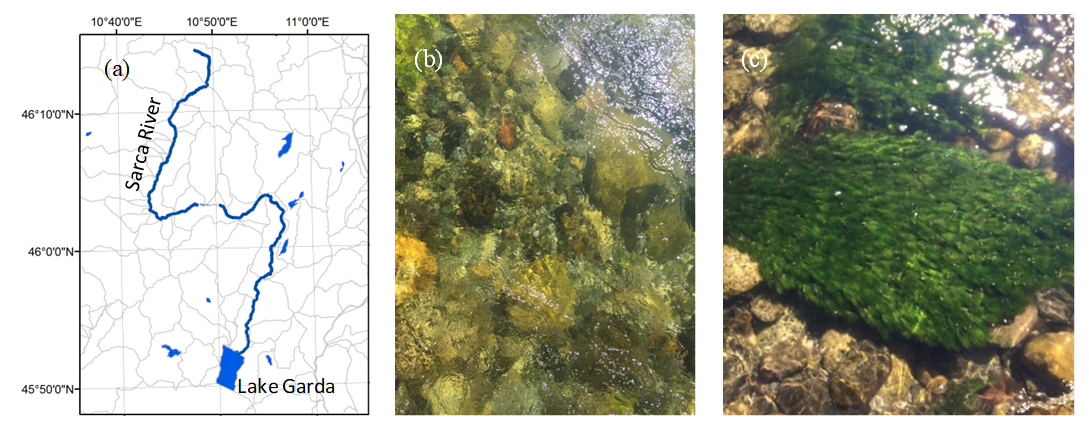
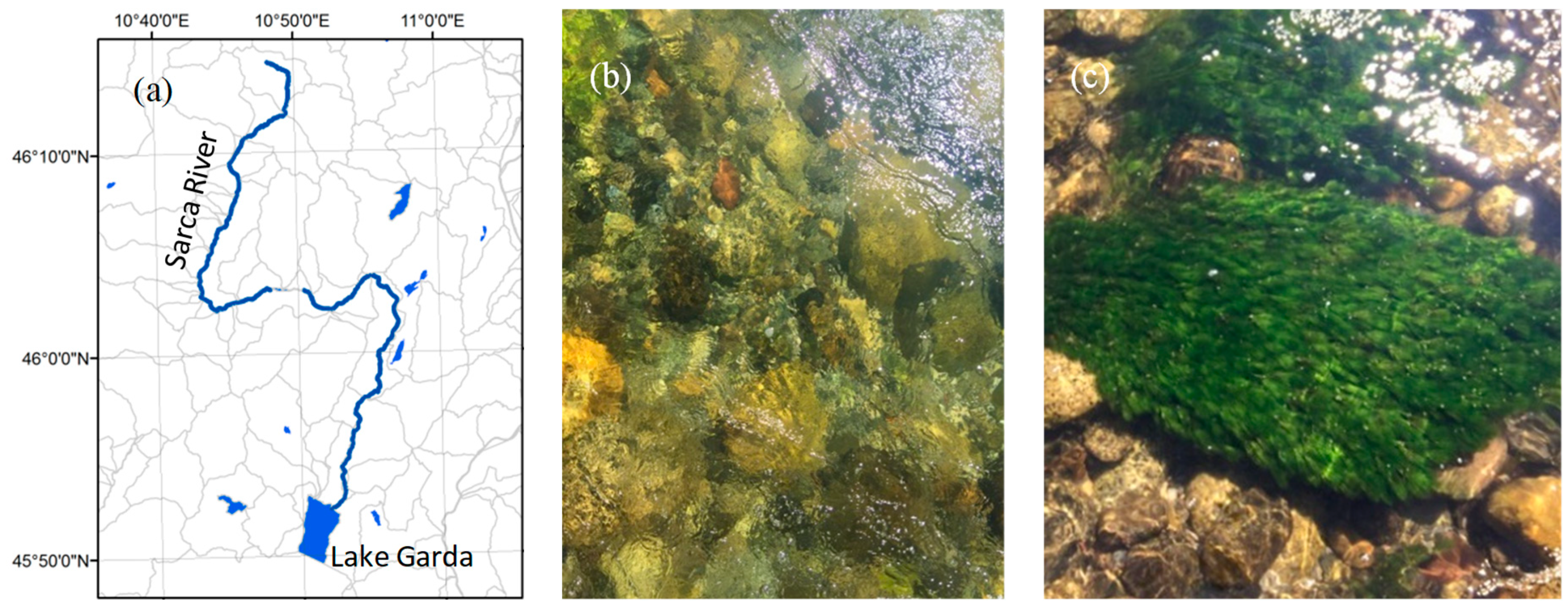
2. Study Area and Datasets

To perform an application-relevant analysis, the three experiments were designed based on the hydro-geomorphological and optical properties of the Sarca River. The Sarca River is a very shallow river in the Italian Alps supplied with meltwater from the Adamello glaciers and flowing into Lake Garda (Figure 1). The riverbed in the study area is composed of gravels (primarily dolomite) with patches of SAV. The mean channel width is about 30 m and the water depth <1 m with an average of about 0.5 m in the study region. The ranges of water column constituents are available from long-term measurements in the study area [25].
To perform a comprehensive assessment of the bottom reflectance retrieval methodology, this study applied three different radiometric datasets: one measured in a laboratory, one simulated using Hydrolight radiative transfer modeling [26], and one collected by the WV3 satellite sensor. The laboratory experiments allowed for controlled measurements of surface reflectance for flowing water with different SAV densities. The simulated spectra enabled an assessment of streambed mapping in a range of bottom types, water depths, and water column constituents representative of a wide range of optical conditions. The multispectral WV3 image of the Sarca River was also used to classify SAV densities to assess the feasibility and effectiveness of water-column correction from space. The measured and simulated reflectances were convolved with spectral responses of WV3 and GeoEye sensors (Table 1).
Table 2 provides a summary of datasets while more details regarding the experiments are provided in Section 4. The constituents are described in terms of concentrations of total suspended sediment (TSS), chlorophyll-a (Chl-a), and the absorption of colored dissolved organic mater at 440 nm (aCDOM (440)).

3. Methods

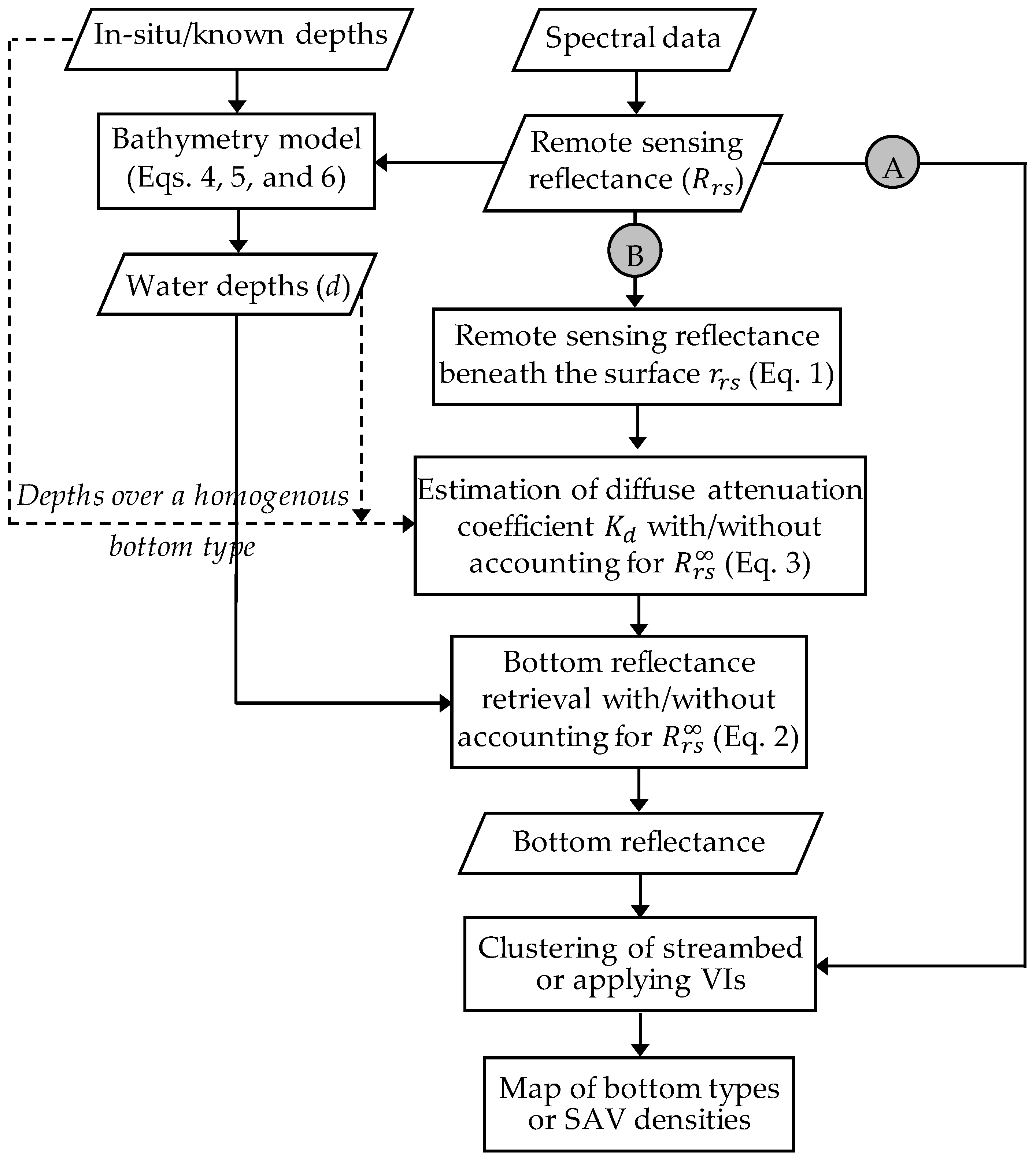
3.1. Water-Column Correction

The early work of Lyzenga [28,29] provided a physical basis for water-column correction and estimation of depth-invariant indices to map bottom properties in coastal settings. A review of bottom mapping techniques developed for remote sensing of coral reefs, algae, and seagrass is provided in [30]. Bottom mapping has been poorly studied in the context of fluvial systems and has mostly been based on above-water reflectances, which neglect the attenuation effects of the water column. The first attempt to apply existing water-column correction techniques in a riverine environment was the work by Legleiter et al. [3] based on limited, field-based spectral measurements. Their results demonstrated that sediment facies and algal densities can be characterized via their spectral information and suggested that retrieving bottom reflectances was not necessary. However, they indicated that the results were based on subjective interpretations of substrate images and suggested that more systematic studies, including radiative transfer modeling, would be needed to explore the potential for bottom reflectance retrieval. This research attempts to employ similar physics-based approaches to map bottom types using spectral reflectance data. In this study, the bottom reflectance retrieval is assisted by estimating K d from image data using known water depths to eliminate the need for field-based spectral measurements carried out by the previous work [3].
The remote sensing reflectance ( R r s ), defined as the ratio of the water-leaving radiance to the total downwelling irradiance just above the water surface, is an apparent optical property critical for analysis of optical imagery over water bodies [31,32,33]. Radiometric and atmospheric corrections are required to derive R r s from top of atmosphere (TOA) radiances [32]. Note that reflectances/radiances and K d are all wavelength (λ)-dependent; however, we drop λ for brevity in the text while retaining it in equations. Remote sensing reflectance just beneath the water surface ( r r s ) can then be estimated to account for transmission and refraction at the air–water interface [3,34]:
r r s ( λ ) = R r s ( λ ) 0.52 + 1.7 R r s ( λ ) .
Thereafter, the remote sensing reflectance of bottom ( r r s B ) can be estimated according to the following equation [3,35,36]:
r r s B ( λ ) = r r s ( λ ) R r s ( λ ) [ 1 e 2 K d ( λ ) d ] e 2 K d ( λ ) d
where R r s denotes the remote sensing reflectance of optically deep water (i.e., negligible bottom-reflected radiance). The parameter K d is the spectral diffuse attenuation coefficient that characterizes the propagation of light through the water column [34]. Legleiter et al. [3] estimated K d by directly measuring a vertical profile of downwelling irradiance within a water column using a spectroradiometer with waterproof accessories. In this study, we solved for K d using water-leaving reflectances observed for different known depths and a homogeneous bottom type adapted from [37,38,39]. For a small reach of river with a homogeneous bottom type, differences in bottom reflectance can be assumed negligible for a given pair of pixels, i.e., r r s B 1 = r r s B 2 . K d can then be estimated by rearranging Equation (2) for each pair of pixels with different water depths (d1, d2):
K d ( λ ) = l n ( r r s 2 ( λ ) R r s ( λ ) r r s 1 ( λ ) R r s ( λ ) ) 2 ( d 1 d 2 ) .
This approach for estimating K d requires R r s coupled with corresponding depth information. Water depth can be measured in the field or inferred from the image. Note that the depth samples for the estimation of K d should be selected from a reach with a uniform substrate. However, the water depth of each individual pixel is required to estimate r r s B (Equation (2)), which can be retrieved from an image using bathymetry models such as Lyzenga’s model [28,29], a band ratio model [40], optimal band ratio analysis (OBRA) [41,42], or multiple optimal depth predictors analysis (MODPA) [13].
We estimated water depths using MODPA, previously developed in the Sarca River, a method that has been proven to provide robust bathymetry retrievals with respect to substrate variability and water column heterogeneity [13]. MODPA initially increases the spectral domain of the original image by adding intensity components from RGB to the hue–saturation–intensity (HSI) transformations. All possible Lyzenga (Equation (4)) and ratio (Equation (5)) predictors of the produced high-dimensional image are then considered as candidate variables for a multiple regression bathymetry model. MODPA selects optimal predictors ( X L y z e n g a _ O p t ,   X R a t i o _ O p t ) among all the candidates based on a feature selection method such as partial least square (PLS) regression to form the bathymetric model (Equation (6)). The unknown parameters of the model (ai, b) can be estimated by performing a multiple regression between m optimal predictors and in-situ depths (d). Note that reflectances can be replaced with radiances in Equations (4) and (5) [12,20] for which R r s was utilized in this study.
X L y z e n g a = l n ( L T ( λ ) L ( λ ) ) , L ( λ ) = L C ( λ ) + L S ( λ ) + L P ( λ )
X R a t i o = l n L T ( λ 1 ) L T ( λ 2 )
d = i = 1 m a i X i + b , X { X L y z e n g a O p t , X R a t i o O p t } .
The radiance observed over optically deep waters ( L ) encompasses upwelling radiance from the water column ( L C ), water surface ( L S ), and atmosphere ( L P ). Subtraction of L from the TOA radiance ( L T ), known as a deep-water correction, isolates the radiance component upwelling from the bottom and can provide information about depth and substrate properties [29,42]. Correctly applying a deep-water correction is challenging in fluvial systems due to the lack of optically deep pixels. However, the effects of deep-water correction become important when the total radiance signal approaches the deep-water signal (i.e., the bottom-reflected signal becomes negligible). In shallow and clear rivers where bottom reflectance makes a larger contribution to the TOA radiance, deep-water correction has been dispensed in some applications such as bathymetric mapping [13,38,43,44]. However, the remote sensing reflectance of optically deep water ( R r s ) is also required to estimate K d and bottom reflectance (Equations (2) and (3)). Legleiter et al. [3] collected spectra from the deepest part of the channel (~2 m deep) to obtain an estimate R r s for performing a water-column correction. However, this assumption is subject to significant uncertainties in clear or very shallow streams where bottom-reflected radiances are dominant. Flener [44] proposed an iterative procedure to estimate L or R r s in shallow rivers that lack optically deep water: L or R r s can initially be estimated using a first-guess and modified in an iterative process such that the correlation between image/spectra-derived quantities (X) and the water depths (d) is maximized. This research has utilized Flener’s method [44] for estimating R r s to assess its impact on retrieval of K d and bottom reflectance.
Figure 2 illustrates the overall workflow for mapping bottom types without and with water-column correction, i.e., using (A) above-water reflectances and (B) retrieved bottom reflectances. The bottom information extracted from these two approaches is then compared to the reference data available from simulations or measured at the laboratory/field. The next subsection describes the methodology for classification of bottom classes and SAV densities.

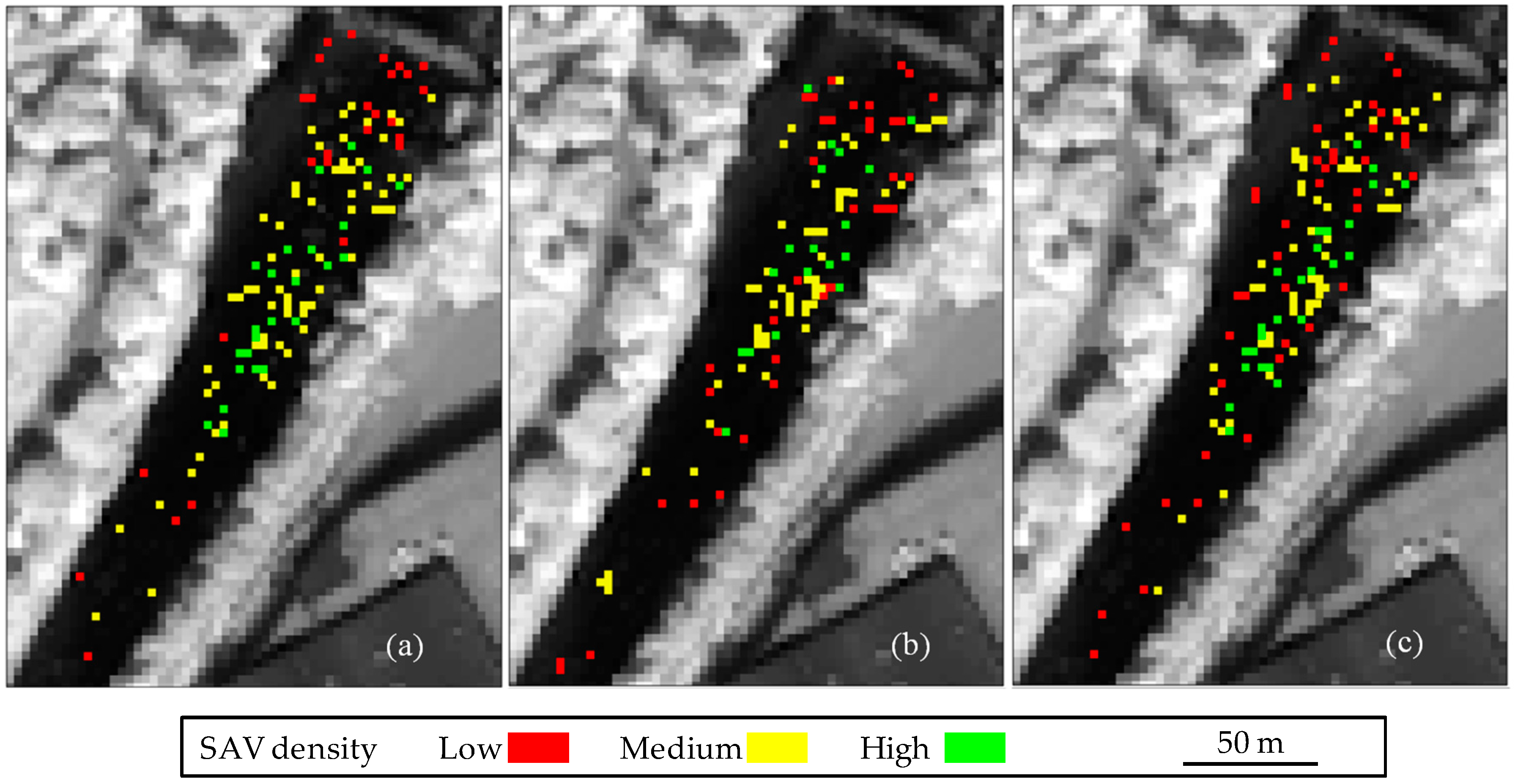
3.2. Classification of Bottom-Type and SAV Densities

The application of supervised classification would be challenging in terms of collecting benthic samples for training the models. To broaden the applicability of our substrate mapping methodology, the k-means algorithm [45], a frequently used unsupervised classifier, was applied to both above-water and retrieved bottom reflectances to map riverbed clusters. The labels were then assigned to the clusters based on interpretation of the spectra associated with the clusters’ centers.
This research also investigates the effectiveness of widely used terrestrial and aquatic vegetation indices (VIs) for detecting and quantifying SAVs in shallow rivers. VIs with different band combinations were examined to identify the SAVs with different densities before and after water-column correction. WV3 is equipped with a red-edge (RE) band and has two NIR bands (NIR1 and NIR2), which collectively allow for evaluating more VIs compared to four-band imagery such as GeoEye data.
The normalized difference vegetation index (NDVI) is a commonly used index [46,47] for examining properties of terrestrial vegetation (Table 3). The attenuation by the water-column, however, can influence the water-leaving radiance to varying degrees depending on depth, bottom properties, and IOPs. More specifically, the sharp increase in reflectance within red to NIR transition spectrum becomes attenuated due to strong pure water absorption in the NIR region [48]. Recently, a water-adjusted vegetation index (WAVI) (see Table 3) has been suggested to account for the background water response [11]. However, this index was developed and tested only in a few lakes. In this study, alternative NDVI and WAVI were computed by replacing the traditional NIR band (~851 nm for GeoEye) with RE and NIR2 bands of WV3 (Table 3).
VIs such as the NDVI are widely used as indicators for fractional vegetation coverage [49,50]. To evaluate the effectiveness of VIs for quantifying SAV densities, using simulated data, regression analyses were performed for various VIs and SAV fractions. In addition, the clustering of VIs to distinguish among SAV density classes was evaluated using laboratory and WV3 data.

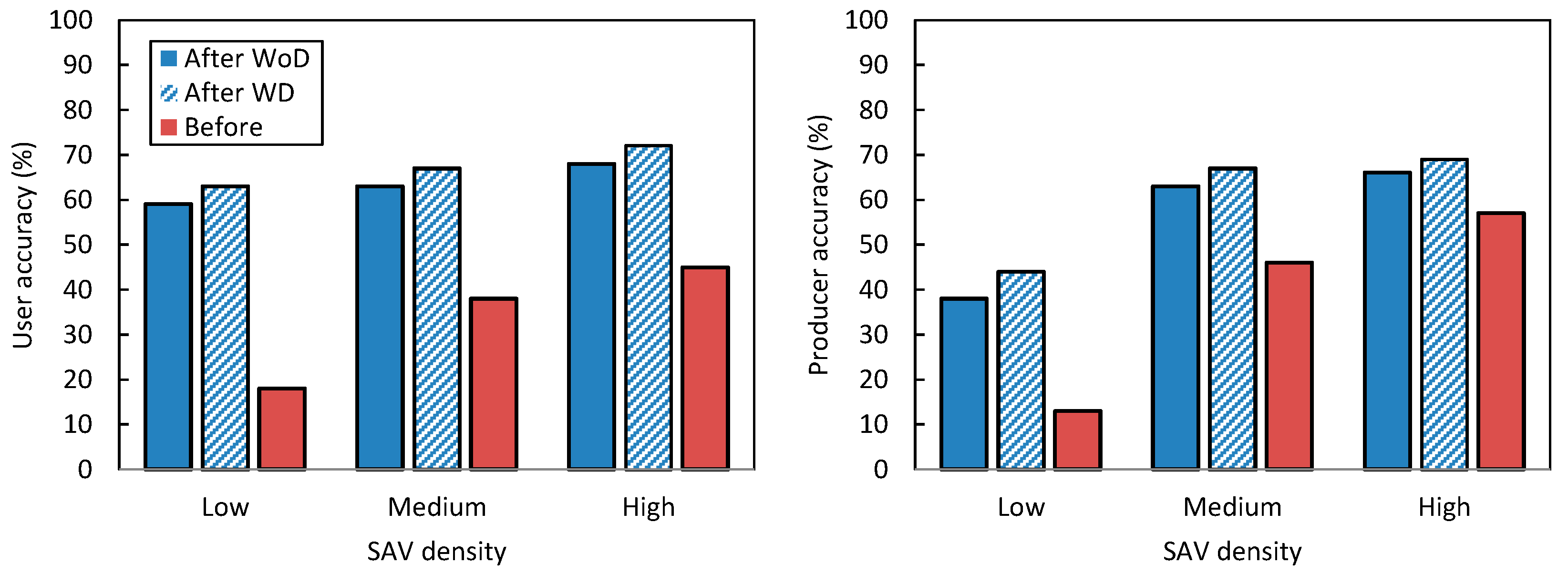
3.3. Accuracy Assessment

The root mean square errors (RMSEs) were calculated to assess the retrievals of bottom reflectance ( R B ) and K d ( R M S E _ R and R M S E _ K d , respectively). Here, we assumed that the bottom is Lambertian for converting the r r s B to the unitless reflectance, i.e., R B = π × r r s B [51]. Note that this assumption is subject to uncertainty due to probable non-Lambertian behavior of the riverbed. However, this does not affect the relative comparison of the spectra as R is a factor of r r s B .
R M S E _ R = i = 1 n ( R B , r e f e r e n c e ( λ i ) R B , r e t r i e v e d ( λ i ) ) 2 n
R M S E _ K d = i = 1 n ( K d r e f e r e n c e ( λ i ) K d r e t r i e v e d ( λ i ) ) 2 n
where the “reference” superscript refers to known parameters from either simulations or measurements. The estimated parameters are denoted by a “retrieved” superscript. n is the number of bands for which visible (λ < 700 nm) and NIR (λ > 700 nm) bands were analyzed separately in this study. Note that R M S E _ R is unitless, while R M S E _ K d has units of 1/m.
Statistics derived from a confusion matrix were also used for the assessment of substrate classes. For a classified map, overall accuracy is the number of correctly classified pixels divided by the total number of pixels. The kappa statistic is a measure of how the classification results compare to class allocations assigned by chance, which is a pessimistic estimation of accuracy. The producer accuracy provides a measure of accuracy for each individual class by calculating the fraction of correctly classified pixels of a given class with respect to the total number of reference pixels for the same class. The user accuracy presents the reliability of each class and is calculated as the fraction of correctly classified pixels of a given class with respect to the total number of pixels labeled as the same class in the classified map [46].

4. Experiments and Results

The K d and bottom reflectance retrieval methods were applied to the datasets described in Section 2 and the associated analyses and results are presented in the following subsections. An overall evaluation of the results is then provided in the discussion section. Note that, hereafter, the spectral parameters are distinguished for each experiment using Lab, Sim and WV3 superscripts for laboratory, simulated, and WV3 data, respectively (e.g., R r s S i m stands for the simulated R r s ).

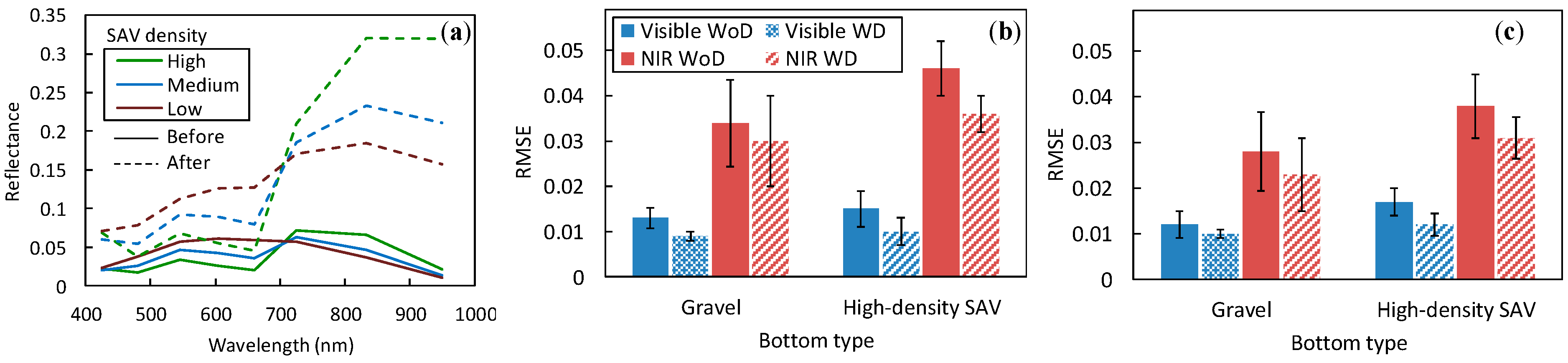
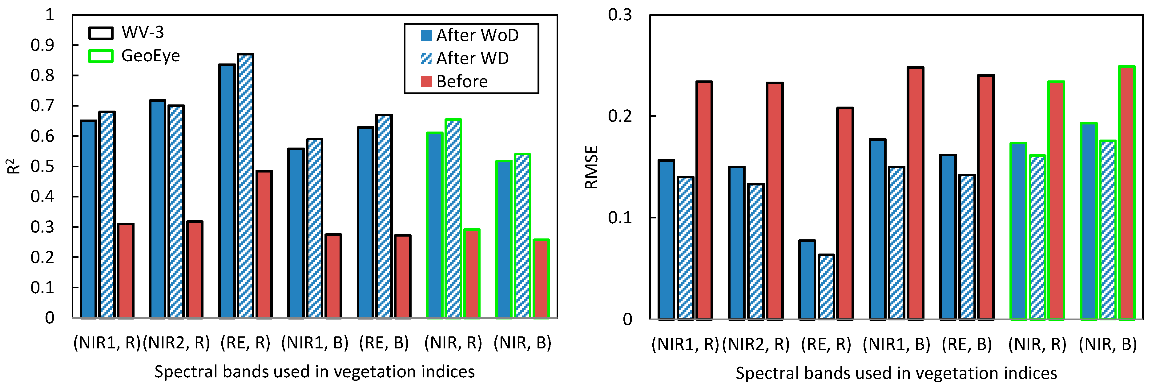
4.1. Laboratory Radiometric Measurements

To quantify water-leaving reflectance under various conditions, including depth and bottom type, spectroscopic measurements were performed in a flume at the University of Trento’s hydraulic laboratory. Spectral reflectance measurements were acquired in a darkroom with an Analytical Spectral Devices (ASD) HandHeld 2 spectroradiometer operating within the 325–1075 nm spectral range. A standard ASD illuminator was used to produce a highly stable light source across the full visible/NIR spectral range. The spectral data were recorded by pointing a fiber optic jumper cable in a near-nadir viewing angle 30 cm above the water surface. The sensor’s field of view was adjusted to sample a cell in the center of the channel to avoid any adjacency effects associated with the flume sidewalls. The illumination geometry was modified to eliminate instrument self-shading over the flume [52]. Three spectra were recorded for each flow condition by averaging 25 individual samples. Radiometric calibrations including white reference and dark current observations were updated before each set of measurements to collect data in reflectance mode.
Four sets of data were collected over different bottom types, including a non-vegetated gravel bed and three SAV densities (high, medium, and low). For each set, dry bottom reflectance (representing exposed material) was first measured as the reference bottom reflectance. Measurements were then continued with 1 cm increments in the water level up to 40 cm. Figure 3 shows the hydraulic flume and the configuration of spectroscopic measurements.
The reflectances ( R L a b ) collected over the water surface were converted to R r s L a b and convolved with GeoEye ( R r s L a b , G ) and WV3 ( R r s L a b , W V 3 ) spectral band passes. R r s L a b along with the bathymetry data collected over a non-vegetated gravel bed were then used to estimate K d (Equation (3)). r r s B was then retrieved using Equation (2).
The above-water reflectances are shown with the associated retrieved bottom reflectances in Figure 4a, allowing for a comparison of 40-cm-deep water at low, medium, and high densities of SAV. The characteristic feature of vegetation is evident on the retrievals of bottom reflectances. However, this feature is significantly attenuated for above-water spectra such that the feature completely disappears for the low-density SAV. The retrieved bottom reflectance showed good agreement (Equations (7) and (8)) with the measured reflectances, particularly across the visible spectrum, and the deep-water correction slightly improved the results (Figure 4b,c). The retrievals from R r s L a b , G (Figure 4c) led to slightly lower RMSEs over the NIR spectrum compared to those from R r s L a b , W V 3 (Figure 4b). This is because WV3 includes an additional band (NIR2; Table 1) spanning over longer NIR wavelengths where pure water absorption is much stronger. The error bars in Figure 4 indicate the effects of the changing water level, i.e., the smaller the error bars, the better the water-column correction. Note that RMSEs have been estimated using five visible bands (λ < 700 nm) and three NIR bands (λ > 700 nm) using R r s L a b , W V 3 . The RMSEs of reflectance retrievals (i.e., R M S E _ R ) for high-density SAV were slightly higher (~0.01) in the NIR spectrum, particularly when the deep-water correction was not applied. This can be attributed to strong attenuation of the vegetation feature in the NIR region caused by pure water absorption. However, deep-water correction mitigated this effect.
Using either above-water spectral measurements R r s L a b or retrieved bottom reflectances r r s B , L a b for various SAV densities, original and alternative NDVIs and WAVIs (Table 3) were computed. The VIs derived from each band combination led to thematic clusters associated with the four SAV densities (see Figure 5; each SAV density is shown with a different color). The thematic clusters of VIs derived from R r s L a b show considerable overlap, which reduces separability among different SAV densities. To further elaborate, the k-means algorithm was applied to VIs to automatically cluster them into four classes. The clusters were ranked based on the average magnitude of the calculated VIs and accordingly were assigned to SAV density classes (i.e., the higher the VI magnitude, the higher the SAV density). The overall accuracies and the kappa coefficients are presented for VIs with different band combinations (Figure 5). The VIs built upon the RE band demonstrated better performance compared to other band combinations using R r s L a b . More specifically, the (RE, R) band combination yielded the highest accuracy with 92% overall accuracy and kappa coefficient of 89%. The aquatic VIs provided no further benefit for clustering SAV densities using R r s L a b . The clusters obtained from r r s B , L a b indicated remarkable distinctions among SAV densities for all the band combinations (Figure 5b). In addition, the clusters are very compact, suggesting minimal impact of varying water depth; this result confirms successful correction of water-column effects. However, these results are based on observations which were limited to a maximum depth of 40 cm with minimal constituent loads (see Table 3). The results based on water-column correction (Figure 5b) are shown only for the case without applying the deep-water correction, as no more enhancements were required for clustering the SAVs.

4.2. Radiative Transfer Simulations

Simulated spectra produced by radiative transfer modeling have been used previously for studying bathymetry retrieval in shallow rivers [12,13,42,53]. Building on this approach, we utilized simulated spectra to gain insight into streambed mapping in shallow riverine environments. To investigate the effectiveness of water-column correction for varying IOPs and bottom types, we simulated the optical properties (Table 2) and generated substrate spectral mixtures for a reach of the Sarca River. The R r s as well as the associated K d were simulated with the widely used Hydrolight radiative transfer model [26,51] for three different bottom types (macrophyte, dark sediment, and dolomite) as well as a range of water column constituents representative of the Sarca River and similar alpine rivers. Maximum and minimum values of the constituents were selected based on long-term observations of water quality indicators documented by local environmental agencies [25]. A database of simulations was produced including more than 20,000 individual spectra (Table 2).
The bathymetry of a reach of the Sarca River was derived from the WV3 image using MODPA [13] and used as a basis for the simulations (Figure 6a). Only a randomly selected 1% of the entire channel depths (about 50 pixels) were used to calibrate the MODPA model and the remaining known depths were reserved for validating the bathymetry model (Figure 6b). The resultant coefficient of determination (R2) of 0.99 and an RMSE of 0.01 m indicated the robustness of the depth retrieval method with respect to the variability in constituents and substrate types within the channel (Figure 6).
The channel was divided into three segments with different concentrations of constituents from clear to turbid water (constituents associated with each of the segments are shown in Figure 7c). Each segment has one dominant bottom type (Figure 7b) but is mixed with up to 50% of two other bottom types. Note that R r s spectra were first simulated considering pure bottom types. The spectra for constant/known water depths (d) and constituents, and only with different bottom types (i.e., R r s B 1 , R r s B 2 and R r s B 3 ), were then mixed linearly [11,54] with the desired fractions ( f 1 , f 2 , f 3 ) to produce the R r s for the simulated channel ( R r s S i m _ C h a n n e l ) according to Equation (9). To generate a reference map for accuracy assessment, each pixel was labeled as the bottom type with the largest fraction (Figure 7b). Figure 7 shows the inputs for simulating the spectra over the river channel. Note that the arrangements of bottom types and constituents within the reaches are just to allocate the simulated spectra to individual pixels so that each reach has a specific optical condition. However, the analyses were performed at the pixel level and independent from the spatial distribution of the pixels.
R r s S i m _ C h a n n e l = f 1 × R r s B 1 + f 2 × R r s B 2 + f 3 × R r s B 3 ,   f 1 + f 2 + f 3 = 1
Furthermore, we examined the performance of K d retrieval in various water-column conditions in the simulated river channel with R r s S i m _ C h a n n e l as the reference. This analysis allowed us to evaluate the effects of variable constituents on the retrievals of K d and r r s B . As required in Equation (3), a number of samples (about 20 pixels) of water depths and the associated R r s S i m _ C h a n n e l were taken from two different test sites: (a) upstream composed of a dominant substrate type of sediment and with a relatively clear water column and (b) downstream with a dominant substrate type of dolomite and relatively turbid waters (Figure 7). The estimations of K d with and without accounting for R r s [44] were compared with the average K d S i m _ C h a n n e l , W V 3 within the entire channel as a reference (Figure 8).
Note that constituents assigned to the downstream area were more representative for the entire simulated stream. Therefore, as expected, downstream estimates of K d were more in agreement with the reference K d S i m _ C h a n n e l (Figure 8) than that of the upstream retrievals, particularly when R r s was not taken into account. Figure 9 shows the RMSEs for upstream and downstream K d retrievals with and without applying deep-water correction. Considering R r s led to improvements in deriving K d , particularly for the upstream-based retrieval.
We utilized the k-means algorithm to perform riverbed classification using R r s S i m _ C h a n n e l and r r s B , S i m _ C h a n n e l . As evident in Figure 10, above-water reflectances ( R r s S i m _ C h a n n e l ) led to a considerable number of misclassified pixels, particularly confusion between the bottom types of the upstream (dominant sediment) and downstream (dominant dolomite) segments. Substrate clusters derived after water-column correction (i.e., using r r s B , S i m _ C h a n n e l ) showed considerably fewer misclassified pixels.
The water-column correction yielded significant improvements (about 20% overall accuracy and 30% kappa coefficient) in mapping bottom types using R r s S i m _ C h a n n e l either for WV3 or GeoEye spectra (Figure 11). Accounting for R r s slightly improved the bottom mapping (~2–3%). Further, downstream K d retrievals yielded slightly better results compared to those of upstream (~2–3%), which implies that substrate mapping was independent of constituent variability in our case study. However, this would probably have considerable effects when detailed spectral information is required for mapping the substrate properties (e.g., bottom types with very similar spectral properties such as different types of SAV) or in the case of highly variable constituents.
To evaluate the effectiveness of VIs for the detection of SAV densities, a regression analysis was performed between known SAV (macrophyte) fractions and associated VIs. The R2 and RMSE for this analysis indicated a significantly stronger correlation between VI and SAV densities after water-column correction (Figure 12). This finding was valid for all band combinations. The strongest correlation was for (RE, R) band combination (Table 1) using either R r s S i m _ C h a n n e l , W V 3 (R2 = 0.48 and RMSE = 0.2) or inferred r r s B , S i m _ C h a n n e l , W V 3 (R2 = 0.85 and RMSE = 0.07). This demonstrated the significance of the WV3’s RE band (i.e., 742 nm) for mapping benthic vegetation in shallow streams, but this band is not available on GeoEye. There is also evidence from studies in wetlands demonstrating the usefulness of the RE band for mapping benthic vegetation but without applying any water-column correction [55,56]. Accounting for R r s slightly improved the regression statistics.
Additional analyses were performed on the database of simulated spectra to examine the effects of water depth and constituents on the bottom reflectance retrieval. Figure 13 (first row) indicates the RMSEs for the inferred bottom reflectances across a range of water depths while holding the constituents constant (TSS = 4 g/m3, Chl-a = 3 mg/m3, and aCDOM (440) = 0.14 m−1). In general, reflectances within the visible bands were retrieved with high accuracies, and the water depth had little effect on RMSEs. The RMSEs for the NIR bands increased sharply with water depth particularly without correcting for R r s . The effect of accounting for R r s was pronounced for relatively deep waters (depth > 0.5 m) and improved the bottom reflectance retrievals, particularly in the NIR spectrum.
In addition, some analyses were performed to investigate the effect of variations in constituent concentration on bottom reflectance retrievals. Three realistic levels of turbidity assumed for the range of constituents in the Sarca River and similar Alpine rivers were considered: low (TSS = 2 g/m3, Chl-a = 1 mg/m3, aCDOM (440) = 0.07 m−1), medium (TSS = 4 g/m3, Chl-a = 3 mg/m3, aCDOM (440) = 0.14 m−1), and high (TSS = 6 g/m3, Chl-a = 5 mg/m3, aCDOM (440) = 0.22 m−1). These constituent conditions are labeled as low, medium, and high turbidity in Figure 13. The effects of constituents were then evaluated in a constant and relatively thick water column (1 m). The RMSE for bottom reflectance retrievals in the NIR bands increased with the increase in turbidity, while the retrievals in the visible bands were less affected. Accounting for R r s improved the retrieval of bottom reflectance, particularly in the NIR bands (see the second row in Figure 13).

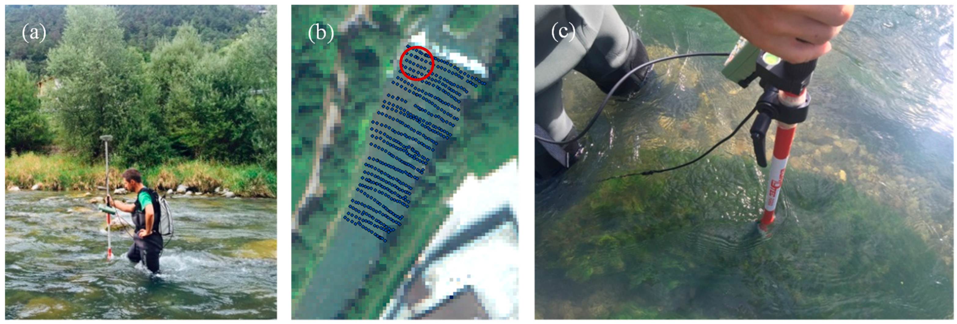
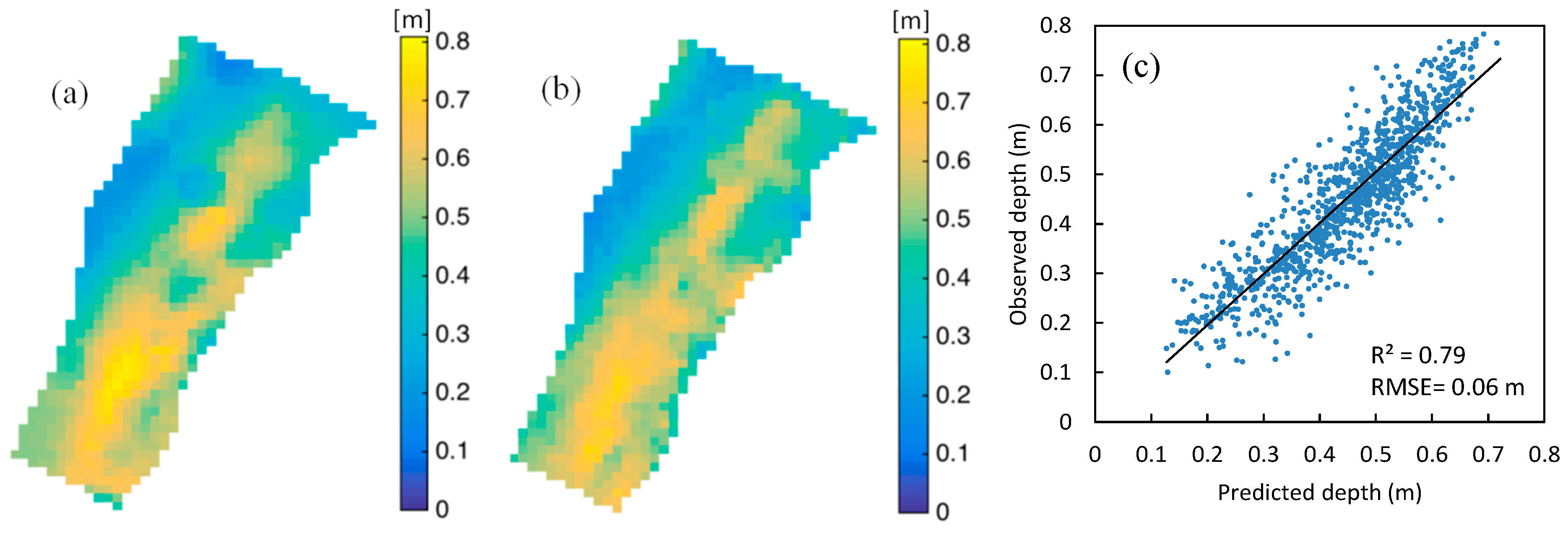
4.3. Image Analysis and Field Survey

To gauge the performance of the bottom reflectance retrieval methodology for SAV-density mapping, we examined an eight-band WV3 image (Table 1) of the Sarca River. The image was acquired on 1 September 2015 with a mean off-nadir view angle of 10.5° and a 1.6 m spatial resolution. In-situ water depths and information on SAV densities were recorded using a real-time-kinematic (RTK) GPS rover (Figure 14). The in-situ depth measurements were conducted along cross sections in three reaches only a few days after image acquisition. Note that the river is regulated by a dam upstream and the water level remained highly stable. The image was delivered georeferenced, but we used control points collected outside the river channel to improve for accurate co-registration of the in-situ data with the image. To link field depths to image pixels, an ordinary kriging was used to interpolate the measured depths at each pixel location [20]. One-half of the data was used for calibration of the MODPA model and the second half as validation for accuracy assessment. For each patch of SAV, approximate areal coverage was documented to further evaluate the performance of clustering SAV-density classes.
A near-simultaneous Landsat-8 image was processed via the SeaWiFS Data Analysis System (SeaDAS) to infer dominant aerosol models over Lake Garda. The eight-band WV3 image of the study area was then atmospherically corrected using the MODerate resolution atmospheric TRANsmission (MODTRAN) code [57,58] to provide R r s W V 3 . K d W V 3 was then estimated using in-situ depths and associated R r s W V 3 (Equation (3)) over a segment of the Sarca River with homogeneous bottom type (shown on Figure 14b). The water-depth map was estimated by calibrating the MODPA model by randomly selecting half of the in-situ depths. The image-derived depth map is shown in Figure 15b for a subset of the river where field observations were carried out (Figure 15a). The validation was performed using the remaining half of the in-situ depths (Figure 15c).
The areal coverage of SAV patches gathered in the field was converted to a density index by dividing the observed area of a patch by the spatial resolution of the image (1.6 × 1.6 m). As a reference map, the index values were clustered using k-means algorithm to three density classes (Figure 16a). The image-derived VIs (either before or after water-column correction) were also clustered using the k-means algorithm and then compared with the reference map. The best results were achieved when the (RE, R) band combination was used both with or without applying water-column correction (Figure 16b,c). These findings are consistent with the results obtained from laboratory and synthetic data analyses.
The user and producer accuracies of SAV-density clusters indicated that the retrieved r r s B , W V 3 yielded remarkably higher accuracies than R r s W V 3 for all the SAV densities. These enhancements were on the order of 22% and 34% in average user and producer accuracies, respectively. Note that accounting for R r s has improved the average user/producer accuracies on the order of 5% for the SAV-density mapping based on r r s B , W V 3 . The accuracies of clustering from R r s W V 3 improved by increasing the SAV density (45% user accuracy and 57% producer accuracy for high-density SAV). This is also valid for clustering from r r s B , W V 3 with a lower magnitude (Figure 17).

5. Discussion

Bottom reflectance retrieval and substrate-type mapping were explored via three independent experiments. The spectroscopic measurements in the hydraulic laboratory and simulations from radiative transfer modeling provided a thorough understanding of the driving factors influencing the feasibility and accuracy of streambed mapping, such as water depth, constituents, deep-water correction, and choices of spectral bands. Further, in a first attempt to map substrate properties from space, an eight-band WV3 image of a reach in the Sarca River was used to classify SAV densities. Results based on spectroscopic measurements and simulations suggest that K d and bottom reflectance retrieval was more accurate in the visible bands than in the NIR bands, particularly for relatively deep waters (>0.5 m). This is attributed to the rapid light attenuation towards longer wavelengths in the NIR region, particularly for thicker water columns. Accounting for deep-water reflectance, R r s was demonstrated to be effective for enhancing retrievals in the NIR spectrum when the water becomes deeper. This result is reasonable, as applying R r s has more of an effect when the bottom-reflected component of the water-leaving radiance approaches zero. However, the effect of R r s was negligible for visible bands in the range of water depths discussed in this study (<1 m) as well as for the NIR bands in very shallow depths (<0.5 m). Further analyses using synthetic data revealed that IOP variability has less impact on r r s B , S i m (bottom reflectance) retrieval in the visible bands. Increasing turbidity reduced the accuracy of r r s B , S i m retrieval in the NIR bands. However, accounting for R r s mitigated the effect of turbidity on retrieval of r r s B , S i m . For instance, R M S E _ R for the macrophyte bottom was reduced ~4X when applying the deep-water correction in highly turbid waters (Figure 13).
As a key finding, water-column correction significantly improved riverbed mapping. For instance, retrieval of r r s B , S i m _ C h a n n e l for three bottom types (dolomite, macrophyte, and sediment) within the simulated channel (Section 4.2) enhanced the riverbed clustering on the order of 20% in overall accuracy and 30% in kappa coefficient compared to classifications obtained from R r s S i m _ C h a n n e l . This was also demonstrated in distinguishing among SAV densities where retrieval of bottom reflectance yielded VIs strongly correlated with macrophyte fractions. The terrestrial VI with (RE, R) band combination was found to provide the highest correlation with the SAV fractions using either r r s B , S i m (R2 = 0.85 and RMSE = 0.07) or R r s S i m (R2 = 0.48 and RMSE = 0.2). The same band combination also yielded the most accurate clusters of SAV densities in analyzing laboratory data as well as the WV3 image. The above-water reflectances ( R r s W V 3 ) showed potentials for detecting high-density SAVs in the Sarca River (user accuracy = 45% and producer accuracy = 57%). This indicates the effectiveness of WV3’s RE band (i.e., 724 nm) for mapping SAVs. Moreover, enhanced spectral resolution of the WV3 compared to the GeoEye provided higher accuracies (on the order of 5%) in mapping the streambed using synthetic data. Note that K d retrievals for the NIR2 band was slightly less accurate than that derived for GeoEye’s NIR band. This can be attributed to the strong water-column attention in the NIR2. Nevertheless, the improved accuracies gained in the clustering experiment using a WV3 image indicated the overall efficacy of enhanced spectral resolution of this sensor compared to the traditional four-band high resolution satellite imagery for mapping bottom compositions. We performed the analyses independent from the spatial resolution in order to isolate the effect of the spectral resolution of sensors. The spatial resolution can also affect the retrieval of bottom reflectances, particularly when there is a high level of mixture in the bed type. However, the effect of spatial resolution would be minor in our case due to comparable spatial resolutions of WV3 and GeoEye imagery.

6. Conclusions and Outlook

Recent research has generated significant optimism regarding the potential of optical remote-sensing imagery to extract key hydro-morphological attributes (e.g. bathymetry) of riverine environments. Understanding and isolating the effect of individual river attributes on the overall spectral response of a water body would reveal valuable information and could enable a wide range of applications in fluvial systems. Although studies of river bathymetry have become relatively mature, little work has been done to explore other essential attributes such as streambed composition. In this research, retrieval of bottom reflectances and mapping riverbed types were addressed. Unlike the bulk of the existing literature [10,17,48], a water-column correction approach was pursued to map bottom properties by retrieving bottom reflectance rather than using above-water spectra. This methodology accounted for water-column attenuation by estimating K d using known depths with a homogeneous bottom type. MODPA was implemented to empirically derive the bathymetry and provided robust depth retrieval. Image-derived depths were then used for estimating K d and then bottom reflectance, so that no in-situ optical measurements were required to obtain K d .
Our attempt to retrieve bottom reflectance from space using WV3 image data, with a focus on mapping SAV densities, demonstrated promising results in a shallow riverine environment. However, further studies are needed to investigate mapping various benthic covers and other substrate attributes (e.g., grain sizes). Sun glint can be a source of uncertainty for mapping bottom types and compositions [59,60]. Imagery affected by sun glint would require pre-processing to reduce the undesirable surface reflections. K d and bottom reflectance retrieval was also facilitated by bathymetric information, which requires some in-situ depth measurements. However, this approach undermines the full potential of streambed mapping when in-situ depth observations are lacking. Theoretical calibration methods of bathymetry models, such as the hydraulically assisted bathymetry model [61], can overcome this problem. Therefore, integration of streambed mapping methodologies with bathymetry models built upon theoretical calibration should be addressed in future studies. The effectiveness of pan-sharpening methods can also be examined in future works in order to further enhance the spatial resolution of streambed mapping using WV3 imagery. Moreover, applications of publicly free Sentinel-2 imagery would be interesting for mapping bottom compositions in large rivers with wider reaches.

Author Contributions

Conceptualization, M.N.J., N.P., and A.V.; Data curation, M.N.J., N.P., and A.V.; Formal analysis, M.N.J.; Methodology, M.N.J. and N.P.; Project administration, M.N.J. and A.V.; Resources, M.N.J. and A.V.; Software, M.N.J.; Validation, M.N.J.; Visualization, M.N.J.; Writing—original draft, M.N.J.; Writing—review & editing, M.N.J., N.P., and A.V.

Funding

Nima Pahlevan was funded under NASA ROSES #NNX16AI16G and the USGS Landsat Science Team Award #140G0118C0011.

Acknowledgments

This work was carried out within the SMART Joint Doctorate (Science for the MAnagement of Rivers and their Tidal systems) funded with the support of the Erasmus Mundus programme of the European Union. The authors gratefully acknowledge ASD Inc. for awarding a short-term usage of HandHeld2 spectroradiometer as of Alexander Goetz Instrument Support program. We are also grateful to Prof. Aronne Armanini, Prof. Maurizio Righetti, and Prof. Guido Zolezzi for giving us access to the hydraulic laboratory.

Conflicts of Interest

The authors declare no conflict of interest.

References

  1. Westaway, R.M.; Lane, S.N.; Hicks, D.M. Remote sensing of clear-water, shallow, gravel-bed rivers using digital photogrammetry. Photogramm. Eng. Remote Sens. 2001, 67, 1271–1281. [Google Scholar]
  2. Woodget, A.S.; Carbonneau, P.E.; Visser, F.; Maddock, I.P. Quantifying submerged fluvial topography using hyperspatial resolution UAS imagery and structure from motion photogrammetry. Earth Surf. Process. Landf. 2015, 40, 47–64. [Google Scholar] [CrossRef]
  3. Legleiter, C.J.; Stegman, T.K.; Overstreet, B.T. Spectrally based mapping of riverbed composition. Geomorphology 2016, 264, 61–79. [Google Scholar] [CrossRef]
  4. Chen, Q.; Yu, R.; Hao, Y.; Wu, L.; Zhang, W.; Zhang, Q.; Bu, X. A New Method for Mapping Aquatic Vegetation Especially Underwater Vegetation in Lake Ulansuhai Using GF-1 Satellite Data. Remote Sens. 2018, 10, 1279. [Google Scholar] [CrossRef]
  5. Lane, S.N.; Widdison, P.E.; Thomas, R.E.; Ashworth, P.J.; Best, J.L.; Lunt, I.A.; Sambrook Smith, G.H.; Simpson, C.J. Quantification of braided river channel change using archival digital image analysis. Earth Surf. Process. Landf. 2010, 35, 971–985. [Google Scholar] [CrossRef]
  6. Strayer, D.L. Submersed vegetation as habitat for invertebrates in the Hudson River estuary. Estuaries Coasts 2007, 30, 253–264. [Google Scholar] [CrossRef]
  7. Dennison, W.C.; Orth, R.J.; Moore, K.A.; Stevenson, J.C.; Carter, V.; Kollar, S.; Bergstrom, P.W.; Batiuk, R.A. Assessing Water Quality with Submersed Aquatic Vegetation. Bioscience 1993, 43, 86–94. [Google Scholar] [CrossRef]
  8. Ghisalberti, M.; Nepf, H.M. The limited growth of vegetated shear layers. Water Resour. Res. 2004, 40. [Google Scholar] [CrossRef] [Green Version]
  9. Flyn, N.J.; Snook, D.L.; Wade, A.J.; Jarvie, H.P. Macrophyte and periphyton dynamics in a UK Cretaceous Chalk stream: The river Kennet, a tributary of the Thames. Sci. Total Environ. 2002, 282–283, 143–157. [Google Scholar] [CrossRef]
  10. Visser, F.; Wallis, C.; Sinnott, A.M. Optical remote sensing of submerged aquatic vegetation: Opportunities for shallow clearwater streams. Limnologica 2013, 43, 388–398. [Google Scholar] [CrossRef] [Green Version]
  11. Villa, P.; Mousivand, A.; Bresciani, M. Aquatic vegetation indices assessment through radiative transfer modeling and linear mixture simulation. Int. J. Appl. Earth Obs. Geoinf. 2014, 30, 113–127. [Google Scholar] [CrossRef]
  12. Legleiter, C.J.; Roberts, D.A. A forward image model for passive optical remote sensing of river bathymetry. Remote Sens. Environ. 2009, 113, 1025–1045. [Google Scholar] [CrossRef]
  13. Niroumand-Jadidi, M.; Vitti, A.; Lyzenga, D.R. Multiple Optimal Depth Predictors Analysis (MODPA) for river bathymetry: Findings from spectroradiometry, simulations, and satellite imagery. Remote Sens. Environ. 2018, 218, 132–147. [Google Scholar] [CrossRef]
  14. Bailly, J.-S.; Le Coarer, Y.; Languille, P.; Stigermark, C.-J.; Allouis, T. Geostatistical estimations of bathymetric LiDAR errors on rivers. Earth Surf. Process. Landf. 2010, 35, 1199–1210. [Google Scholar] [CrossRef]
  15. Mandlburger, G.; Hauer, C.; Wieser, M.; Pfeifer, N. Topo-Bathymetric LiDAR for Monitoring River Morphodynamics and Instream Habitats—A Case Study at the Pielach River. Remote Sens. 2015, 7, 6160–6195. [Google Scholar] [CrossRef] [Green Version]
  16. Niroumand-Jadidi, M.; Vitti, A. Grain size mapping in shallow rivers using spectral information: A lab spectroradiometry perspective. Proc. SPIE 2017, 10422, 104220B. [Google Scholar]
  17. Flynn, K.; Chapra, S. Remote Sensing of Submerged Aquatic Vegetation in a Shallow Non-Turbid River Using an Unmanned Aerial Vehicle. Remote Sens. 2014, 6, 12815–12836. [Google Scholar] [CrossRef] [Green Version]
  18. Anker, Y.; Hershkovitz, Y.; Ben Dor, E.; Gasith, A. Application of aerial digital photography for macrophyte cover and composition survey in small rural streams. River Res. Appl. 2014, 30, 925–937. [Google Scholar] [CrossRef]
  19. Marcus, W.A.; Fonstad, M.A. Optical remote mapping of rivers at sub-meter resolutions and watershed extents. Earth Surf. Process. Landf. 2008, 33, 4–24. [Google Scholar] [CrossRef]
  20. Legleiter, C.J.; Overstreet, B.T. Mapping gravel-bed river bathymetry from space. J. Geophys. Res. 2012, 117, 82071. [Google Scholar] [CrossRef]
  21. Hugue, F.; Lapointe, M.; Eaton, B.C.; Lepoutre, A. Satellite-based remote sensing of running water habitats at large riverscape scales: Tools to analyze habitat heterogeneity for river ecosystem management. Geomorphology 2016, 253, 353–369. [Google Scholar] [CrossRef]
  22. Niroumand-Jadidi, M.; Vitti, A. Reconstruction of river boundaries at sub-pixel resolution: Estimation and spatial allocation of water fractions. ISPRS Int. J. Geo-Inf. 2017, 6, 383. [Google Scholar] [CrossRef]
  23. Niroumand-Jadidi, M.; Vitti, A. Improving the accuracies of bathymetric models based on multiple regression for calibration (case study: Sarca River, Italy). Proc. SPIE 2016, 9999, 99990Q. [Google Scholar] [CrossRef]
  24. Belward, A.S.; Skøien, J.O. Who launched what, when and why; trends in global land-cover observation capacity from civilian earth observation satellites. ISPRS J. Photogramm. Remote Sens. 2015, 103, 115–128. [Google Scholar] [CrossRef] [Green Version]
  25. Giardino, C.; Brando, V.E.; Dekker, A.G.; Strömbeck, N.; Candiani, G. Assessment of water quality in Lake Garda (Italy) using Hyperion. Remote Sens. Environ. 2007, 109, 183–195. [Google Scholar] [CrossRef]
  26. Mobley, C.D.; Sundman, L.K. Hydrolight 5.2 Ecolight 5.2 Users’ Guide; Sequoia Scientific, Inc.: Bellevue, WA, USA, 2008. [Google Scholar]
  27. DigitalGlobe. Spectral Response for DigitalGlobe Earth Imaging Instruments; DigitalGlobe: Westminster, CO, USA, 2013. [Google Scholar]
  28. Lyzenga, D.R. Passive remote sensing techniques for mapping water depth and bottom features. Appl. Opt. 1978, 17, 379. [Google Scholar] [CrossRef]
  29. Lyzenga, D.R. Remote sensing of bottom reflectance and water attenuation parameters in shallow water using aircraft and Landsat data. Int. J. Remote Sens. 1981, 2, 71–82. [Google Scholar] [CrossRef]
  30. Zoffoli, M.L.; Frouin, R.; Kampel, M. Water Column Correction for Coral Reef Studies by Remote Sensing. Sensors 2014, 14, 16881–16931. [Google Scholar] [CrossRef] [PubMed] [Green Version]
  31. Mobley, C.D. Estimation of the remote-sensing reflectance from above-surface measurements. Appl. Opt. 1999, 38, 7442. [Google Scholar] [CrossRef] [PubMed]
  32. Mobley, C.D.; Sundman, L.K.; Davis, C.O.; Bowles, J.H.; Downes, T.V.; Leathers, R.A.; Montes, M.J.; Bissett, W.P.; Kohler, D.D.R.; Reid, R.P.; et al. Interpretation of hyperspectral remote-sensing imagery by spectrum matching and look-up tables. Appl. Opt. 2005, 44, 3576–3592. [Google Scholar] [CrossRef]
  33. Pahlevan, N.; Schott, J.R.; Franz, B.A.; Zibordi, G.; Markham, B.; Bailey, S.; Schaaf, C.B.; Ondrusek, M.; Greb, S.; Strait, C.M. Landsat 8 remote sensing reflectance (Rrs) products: Evaluations, intercomparisons, and enhancements. Remote Sens. Environ. 2017, 190, 289–301. [Google Scholar] [CrossRef]
  34. Lee, Z.; Carder, K.L.; Arnone, R.A. Deriving inherent optical properties from water color: A multiband quasi-analytical algorithm for optically deep waters. Appl. Opt. 2002, 41, 5755–5772. [Google Scholar] [CrossRef] [PubMed]
  35. Maritorena, S.; Morel, A.; Gentili, B. Diffuse reflectance of oceanic shallow waters: Influence of water depth and bottom albedo. Limnol. Oceanogr. 1994, 39, 1689–1703. [Google Scholar] [CrossRef] [Green Version]
  36. O’Neill, J.D.; Costa, M.; Sharma, T. Remote Sensing of Shallow Coastal Benthic Substrates: In situ Spectra and Mapping of Eelgrass (Zostera marina) in the Gulf Islands National Park Reserve of Canada. Remote Sens. 2011, 3, 975–1005. [Google Scholar] [CrossRef] [Green Version]
  37. MARITORENA, S. Remote sensing of the water attenuation in coral reefs: A case study in French Polynesia. Int. J. Remote Sens. 1996, 17, 155–166. [Google Scholar] [CrossRef]
  38. Mumby, P.; Edwards, A. Water Column Correction Techniques. In Remote Sensing Handbook for Tropical Coastal Management; UNESCO: Paris, France, 2000; pp. 121–128. ISBN 92-3-103736-6. [Google Scholar]
  39. Fritz, C.; Dörnhöfer, K.; Schneider, T.; Geist, J.; Oppelt, N. Mapping Submerged Aquatic Vegetation Using RapidEye Satellite Data: The Example of Lake Kummerow (Germany). Water 2017, 9, 510. [Google Scholar] [CrossRef]
  40. Stumpf, R.P.; Holderied, K.; Sinclair, M. Determination of water depth with high-resolution satellite imagery over variable bottom types. Limnol. Oceanogr. 2003, 48, 547–556. [Google Scholar] [CrossRef] [Green Version]
  41. Niroumand-Jadidi, M.; Vitti, A. Optimal band ratio analysis of WorldView-3 imagery for bathymetry of shallow rivers (case study: Sarca River, Italy). Available online: https://www.researchgate.net/publication/304343285_OPTIMAL_BAND_RATIO_ANALYSIS_OF_WORLDVIEW-3_IMAGERY_FOR_BATHYMETRY_OF_SHALLOW_RIVERS_CASE_STUDY_SARCA_RIVER_ITALY (accessed on 28 January 2019).
  42. Legleiter, C.J.; Roberts, D.A.; Lawrence, R.L. Spectrally based remote sensing of river bathymetry. Earth Surf. Process. Landf. 2009, 34, 1039–1059. [Google Scholar] [CrossRef] [Green Version]
  43. Flener, C.; Lotsari, E.; Alho, P.; Käyhkö, J. Comparison of empirical and theoretical remote sensing based bathymetry models in river environments. River Res. Appl. 2012, 28, 118–133. [Google Scholar] [CrossRef]
  44. Flener, C. Estimating Deep Water Radiance in Shallow Water: Adapting Optical Bathymetry Modelling to Shallow River Environments. Boreal Environ. Res. 2013, 18, 488–502. [Google Scholar]
  45. Hartigan, J.A.; Wong, M.A. Algorithm AS 136: A K-Means Clustering Algorithm. Appl. Stat. 1979, 28, 100. [Google Scholar] [CrossRef]
  46. Jensen, J.R. Introductory Digital Image Processing: A Remote Sensing Perspective; Prentice Hall: Upper Saddle River, NJ, USA, 2005; ISBN 0131453610. [Google Scholar]
  47. Cho, H.J.; Mishra, D.; Wood, J. Remote Sensing of Submerged Aquatic Vegetation. In Remote Sensing—Applications; InTech: Rijeka, Croatia, 2012; ISBN 9789535106517. [Google Scholar] [Green Version]
  48. Hedley, J.D.; Roelfsema, C.M.; Phinn, S.R.; Mumby, P.J.; Hedley, J.D.; Roelfsema, C.M.; Phinn, S.R.; Mumby, P.J. Environmental and Sensor Limitations in Optical Remote Sensing of Coral Reefs: Implications for Monitoring and Sensor Design. Remote Sens. 2012, 4, 271–302. [Google Scholar] [CrossRef] [Green Version]
  49. Hurcom, S.J.; Harrison, A.R. The NDVI and spectral decomposition for semi-arid vegetation abundance estimation. Int. J. Remote Sens. 1998, 19, 3109–3125. [Google Scholar] [CrossRef]
  50. Elmore, A.J.; Mustard, J.F.; Manning, S.J.; Lobell, D.B. Quantifying Vegetation Change in Semiarid Environments: Precision and Accuracy of Spectral Mixture Analysis and the Normalized Difference Vegetation Index. Remote Sens. Environ. 2000, 73, 87–102. [Google Scholar] [CrossRef]
  51. Mobley, C.D. Light and Water: Radiative Transfer in Natural Waters; Academic Press: San Diego, CA, USA, 1994; ISBN 9780125027502. [Google Scholar]
  52. Gordon, H.R.; Ding, K. Self-shading of in-water optical instruments. Limnol. Oceanogr. 1992, 37, 491–500. [Google Scholar] [CrossRef] [Green Version]
  53. Niroumand-Jadidi, M.; Bovolo, F.; Vitti, A.; Bruzzone, L. A novel approach for bathymetry of shallow rivers based on spectral magnitude and shape predictors using stepwise regression. In Image and Signal Processing for Remote Sensing XXIV; Bruzzone, L., Bovolo, F., Benediktsson, J.A., Eds.; SPIE Remote Sensing: Berlin, Germany, 2018; Volume 10789, p. 23. [Google Scholar]
  54. Legleiter, C.J.; Roberts, D.A. Effects of channel morphology and sensor spatial resolution on image-derived depth estimates. Remote Sens. Environ. 2005, 95, 231–247. [Google Scholar] [CrossRef] [Green Version]
  55. Lane, C.; Liu, H.; Autrey, B.; Anenkhonov, O.; Chepinoga, V.; Wu, Q.; Lane, C.R.; Liu, H.; Autrey, B.C.; Anenkhonov, O.A.; et al. Improved Wetland Classification Using Eight-Band High Resolution Satellite Imagery and a Hybrid Approach. Remote Sens. 2014, 6, 12187–12216. [Google Scholar] [CrossRef] [Green Version]
  56. Whiteside, T.G.; Bartolo, R.E. Mapping Aquatic Vegetation in a Tropical Wetland Using High Spatial Resolution Multispectral Satellite Imagery. Remote Sens. 2015, 7, 11664–11694. [Google Scholar] [CrossRef] [Green Version]
  57. Berk, A.; Anderson, G.P.; Acharya, P.K.; Bernstein, L.S.; Muratov, L.; Lee, J.; Fox, M.; Adler-Golden, S.M.; Chetwynd, J.H., Jr.; Hoke, M.L.; et al. MODTRAN5: 2006 Update; Shen, S.S., Lewis, P.E., Eds.; International Society for Optics and Photonics: Orlando, FL, USA, 2006; Volume 6233, p. 62331F. [Google Scholar]
  58. Pahlevan, N.; Lee, Z.; Wei, J.; Schaaf, C.B.; Schott, J.R.; Berk, A. On-orbit radiometric characterization of OLI (Landsat-8) for applications in aquatic remote sensing. Remote Sens. Environ. 2014, 154, 272–284. [Google Scholar] [CrossRef]
  59. Carbonneau, P.E.; Lane, S.N.; Bergeron, N. Feature based image processing methods applied to bathymetric measurements from airborne remote sensing in fluvial environments. Earth Surf. Process. Landf. 2006, 31, 1413–1423. [Google Scholar] [CrossRef]
  60. Overstreet, B.T.; Legleiter, C.J. Removing sun glint from optical remote sensing images of shallow rivers. Earth Surf. Process. Landf. 2017, 42, 318–333. [Google Scholar] [CrossRef]
  61. Fonstad, M.A.; Marcus, W.A. Remote sensing of stream depths with hydraulically assisted bathymetry (HAB) models. Geomorphology 2005, 72, 320–339. [Google Scholar] [CrossRef]
Figure 1. (a) The Sarca River located in Northeast Italy and main bottom types including (b) gravels composed of dolomite and (c) patches of submerged aquatic vegetation (SAV).
Remotesensing 11 00262 g001
Figure 2. Flowchart for streambed mapping and delineation of SAV (A) before and (B) after water-column correction. The depth information required for K d estimations can be collected either in the field or derived from image/spectra (shown by dashed lines).
Remotesensing 11 00262 g002
Figure 3. (a) The setup for spectroscopic experiments on the hydraulic flume and the spectral measurements of (b) SAV with high density and (c) the white reference. The spectral reflectances were recorded from above the water surface within the 325–1075 nm range using a fiber optic cable connected to an ASD HandHeld 2 spectroradiometer.
Remotesensing 11 00262 g003
Figure 4. (a) Spectra characterized by different SAV densities before and after water-column correction ( R r s L a b , W V 3 vs. r r s B , W V 3 ). RMSEs for the retrieved bottom reflectances (unitless) with (WD) and without (WoD) applying deep-water correction across visible and NIR bands (Equation (7)) using (b) R r s L a b , W V 3 and (c) R r s L a b , G . Error bars (standard deviation of R M S E _ R ) indicate the effect of variable water depth.
Remotesensing 11 00262 g004
Figure 5. Evaluating the effectiveness of VIs in clustering SAVs with different densities in laboratory experiments. k-means clustering is applied on VIs with different band combinations (a) before and (b) after water-column correction. Zero-density SAVs stand for non-vegetated gravel bed. OA: overall accuracy; K: kappa coefficient.
Remotesensing 11 00262 g005
Figure 6. (a) The bathymetry map retrieved for the simulated channel using R r s S i m _ C h a n n e l , W V 3 and (b) match-up validation.
Remotesensing 11 00262 g006
Figure 7. Inputs for simulation of spectra across the river channel ( R r s S i m _ C h a n n e l ) associated with (a) water depths in a reach of the Sarca River considering (b) dominant bottom types, (c) variable constituents, and (df) fractions of bottom types. A linear mixture model (Equation (9)) was applied to account for the variability (fractions) of bottom types within the pixels. Two test sites used for the estimation of K d are highlighted by circles on the first graph.
Remotesensing 11 00262 g007
Figure 8. Retrievals of K d for the simulated river channel (a) without and (b) with accounting for R r s compared to the reference K d S i m _ C h a n n e l , W V 3 .
Remotesensing 11 00262 g008
Figure 9. Performance of K d retrievals expressed in terms of RMSE (1/m) using (a) R r s S i m _ C h a n n e l , W V 3 and (b) R r s S i m _ C h a n n e l , G by sampling the depths from upstream and downstream of the simulated channel with (WD) and without (WoD) accounting for deep-water reflectance R r s .
Remotesensing 11 00262 g009
Figure 10. Clustering of bed-types for simulated channel before and after water-column correction (i.e., using R r s S i m _ C h a n n e l and r r s B , S i m _ C h a n n e l , respectively) by sampling the pixels required for K d retrieval from upstream.
Remotesensing 11 00262 g010aRemotesensing 11 00262 g010b
Figure 11. The overall accuracies and kappa coefficients of the bottom maps before and after water-column correction. The statistics are presented for upstream (Up) and downstream (Down) K d retrievals for WV3 and GeoEye spectra. The accuracies with applying deep-water correction are shown by hatched bars.
Remotesensing 11 00262 g011
Figure 12. R2 and RMSE of regressions between VIs and SAV fractions before and after water-column correction with (WD) and without (WoD) accounting for deep-water reflectance R r s .
Remotesensing 11 00262 g012
Figure 13. RMSEs (unitless) of reflectance retrievals using the database of R r s S i m _ W V 3 for three bottom types by isolating the effect of water depth (constant constituents: TSS = 4 g/m3, Chl-a = 3 mg/m3, aCDOM (440) = 0.14 m−1) and the effect of constituents (constant 1 m deep water) with (WD) and without (WoD) accounting for deep-water reflectance R r s .
Remotesensing 11 00262 g013aRemotesensing 11 00262 g013b
Figure 14. (a) Field observations to record water depths and SAV densities assisted by a precise RTK GPS, (b) cross-sectional measurement points of water-depths superimposed on the WV3 image, and (c) a sample of SAV in the Sarca River. The sampling area used for estimation of K d is highlighted by a circle on the satellite image.
Remotesensing 11 00262 g014
Figure 15. (a) In-situ depths compared to (b) MODPA-derived depth map of the Sarca River and (c) match-up validation.
Remotesensing 11 00262 g015
Figure 16. (a) In-situ map of SAV densities compared to the maps derived from clustering of the VI with (RE, R) band combination (b) before and (c) after water-column correction using the WV3 image.
Remotesensing 11 00262 g016
Figure 17. User and producer accuracies of SAV density clusters derived from WV3 image based on VI (RE, R) before and after water-column correction with (WD) and without (WoD) accounting for deep-water reflectance, R r s .
Remotesensing 11 00262 g017
Table 1. Multispectral band designations for GeoEye and WV3 sensors [27].
GeoEyeWV3
BandCenter Wavelength
(nm)
Bandwidth
(nm)
BandCenter Wavelength
(nm)
Bandwidth
(nm)
Blue (B)48476Coastal-Blue (CB)42660
Green (G)54781Blue (B)48172
Red (R)67642Green (G)54779
NIR851156Yellow (Y)60549
Red (R)66170
Red Edge (RE)72451
NIR1832134
NIR2948182
Table 2. Datasets used in this study and their specifications.
DatasetSpectral CharacteristicsBottom TypesWater DepthsConstituents
LaboratorySpectroradiometric data with 1 nm resolution convolved to WV3 and GeoEye bandsNon-vegetated gravel, SAV with different densities0 to 0.4 m with 1 cm intervalsClear water with low TSS (~2 g/m3)
SyntheticHydrolight simulations with 10 nm resolution convolved to WV3 and GeoEye bandsSediment, Macrophyte and Dolomite0 to 1 m with 2 cm intervalsTSS = 2–6 g/m3
Chl-a = 1–5 mg/m3
aCDOM (440) = 0.07–0.22 m−1
Satellite8-band WV3 imageSAV with different densities0 to 0.8 mTSS ~ 3 g/m3
Chl-a ~ 2 mg/m3
aCDOM (440) ~ 0.09 m−1
Table 3. Vegetation indices (VIs) used to study SAV.
VIsOriginal FormulaAlternative WV3 Band Combinations
Terrestrial W A V I = R N I R R R R N I R + R R (NIR1, R), (NIR2, R), (RE, R)
Aquatic W A V I = 1.5 R N I R R B R N I R + R B + 0.5 (NIR1, B), (RE, B)

