Resolving Three-Dimensional Surface Motion with InSAR: Constraints from Multi-Geometry Data Fusion

Abstract

Interferometric synthetic aperture radar (InSAR) technology has been widely applied to measure Earth surface motions related to natural and anthropogenic crustal deformation phenomena. With the widespread uptake of data captured by the European Space Agency’s Sentinel-1 mission and other recently launched or planned space-borne SAR missions, the usage of the InSAR technique to detect and monitor Earth surface displacements will increase even more in the coming years. However, InSAR can only measure a one-dimensional motion along the radar line of sight (LOS), which makes interpretation and communication of InSAR measurements challenging, and can add ambiguity to the modelling process. Within this paper, we investigate the implications of the InSAR LOS geometry using simulated and observed deformation phenomena and describe a methodology for multi-geometry data fusion of LOS InSAR measurements from many viewing geometries. We find that projecting LOS measurements to the vertical direction using the incidence angle of the satellite sensor (and implicitly assuming no horizontal motions are present) may result in large errors depending on the magnitude of horizontal motion and on the steepness of the incidence angle. We quantify these errors as the maximum expected error from simulated LOS observations based on a Mogi deformation model. However, we recommend to use LOS observations from several image geometries wherever data are available, in order to solve for vertical and E–W oriented horizontal motion. For an anthropogenic deformation phenomenon observed in seven independent InSAR analyses of Envisat SAR data from the Sydney region, Australia, we find that the strong horizontal motion present could lead to misinterpretation of the actual motion direction when projecting LOS measurements to vertical (uplift instead of subsidence). In this example, the difference between multi-geometry data fusion and vertical projection of LOS measurements (at an incidence angle of 33.8°) reach up to 67% of the maximum vertical displacement rate. Furthermore, the position of maximum vertical motion is displaced horizontally by several hundred metres when the LOS measurements are projected.

1. Introduction

In the past three decades, InSAR has proven to be a valuable geodetic technique to detect and quantify motion of the Earth’s surface (either defined as a displacement or a displacement rate, aka velocity). In contrast to other geodetic techniques, InSAR can image large areas giving a high spatial resolution of measurement points. Time series InSAR analysis allows us to accurately measure surface motions at the millimetre to centimetre scale at a subset of pixels with consistent backscattering characteristics (e.g., [1,2,3,4,5]). A major limitation of InSAR is that the resulting motion measurements are restricted to a one-dimensional (1D) line of sight (LOS) viewing geometry. However, surface motions (resulting from subsurface deformation processes) generally occur in the three spatial dimensions (i.e., east (E), north (N) and up (U)). This means that the InSAR analysis of a stack of synthetic aperture radar (SAR) images acquired in a single viewing geometry is not able to fully capture the magnitude and direction of surface motions (e.g., [6], p. 163). As a consequence, these LOS measurements are hard to interpret and communicate to stakeholders unfamiliar with the concept of a 1D viewing geometry. For this reason, InSAR-derived LOS measurements are interpreted as vertical deformation in some studies without discussing the horizontal contribution to the original measurements (e.g., [7,8,9,10,11,12]). In many scientific and commercial studies LOS measurements are converted into the vertical direction by projecting the data using the sensor incidence angle. This procedure neglects the horizontal components of motion that would also be mapped into the LOS. The assumption of a purely vertical motion field is mentioned in most of these studies (e.g., [13,14,15,16,17,18,19,20,21,22,23,24,25,26,27,28,29,30,31]). However, some studies apply the projection of LOS to vertical without stating the assumption of no horizontal motion occurring (e.g., [32,33,34,35,36,37,38]). In general, the LOS to vertical projection is usually only valid for specific parts of a deforming area (e.g., the centre of a subsidence bowl). For certain crustal deformation mechanisms, the horizontal components of motion can be even larger than the vertical component, depending on position within the deformation field and on the SAR sensor’s incidence angle. To the authors’ knowledge, the error made when projecting LOS to vertical and neglecting any horizontal motion has not yet been quantified with observations.

Previous works have already emphasised the importance of combining multi-geometry InSAR data sets to accurately retrieve the local displacement field (e.g., [39,40,41]). When InSAR observations from both ascending and descending satellite passes are available, it is possible to combine LOS displacements to separate the vertical component from one horizontal component (usually E–W) (e.g., [42,43,44,45]). In many cases the N–S component cannot be separated because it is poorly constrained by the satellite geometry (see Section 4.1), even when data is acquired in both left- and right-looking imaging modes. However, for large motion events (at the metre-scale) it is possible to recover the full 3D motion field by combining conventional InSAR with motion in the azimuth direction derived from the pixel offset tracking or multi-aperture interferometry approaches [46,47,48,49,50,51]. Different approaches to resolve 3D surface motion from InSAR data are reviewed in reference [52], with the conclusion that a particular approach should be chosen according to the type of deformation and the available InSAR and other geodetic data. If independent geodetic data sources are available, such as GNSS (Global Navigation Satellite Systems) measurements, the horizontal motion can be constrained by these data sets in order to extract vertical motion from the InSAR LOS signal. This is particularly applicable when a long wavelength deformation signal is the target of investigation because the relatively sparse sampling of GNSS measurements is less of an issue when the deformation signal has a long wavelength [53,54,55,56]. Furthermore, independent geodetic data can be used to solve for a full 3D motion vector by combining the data sets mathematically on a pixel-by-pixel basis [57,58,59,60,61,62].

In this paper we conduct an investigation into the implications of the LOS geometry of InSAR measurements and the fusion of ascending and descending LOS measurements using simulated and observed deformation phenomena. The paper will address the following questions:

• What magnitude of error is made when projecting LOS to vertical and neglecting the possibility of horizontal motion?
• How can we rigorously estimate vertical and horizontal surface motions from the InSAR LOS geometry?
• Can we solve for the N–S component of motion using a multi-geometry data fusion of InSAR LOS measurements (without using the less precise pixel offset tracking or multi-aperture interferometry methods, independent geodetic data sources or data from right- and left-looking geometries)?

To answer these questions, we use a simulated deformation field based on a Mogi model [63] and an observed deformation field captured by Envisat SAR data across seven different viewing geometries. In Section 2, we present the theory on rigorous estimation of vertical and horizontal surface motions from LOS InSAR data measured in multiple viewing geometries. The simulated deformation case is presented in Section 3, and the observed data case in Section 4. The paper finishes with a discussion of the findings and some major conclusions.

2. Methods

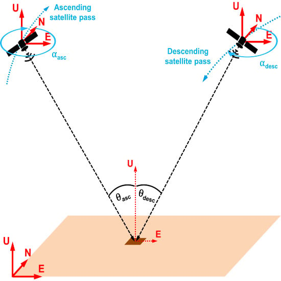
2.1. InSAR Line of Sight Viewing Geometry

The viewing geometry of the satellite LOS is defined by incidence angle $\theta$ (the angle between the local zenith and the looking vector of the satellite) and satellite heading $\alpha$. The LOS observations are made in a direction orthogonal to the satellite heading, with all simulated and real data used in this paper being acquired in a right-looking imaging geometry relative to the heading (see Figure 1). In what follows we describe surface motions in terms of displacement rate (aka velocity), though the same description holds for discrete displacements. A LOS velocity $v_{LOS}$ is composed of the 3D velocity components $v_E$, $v_N$, $v_U$ (e.g., [46] or [6], p. 162):

$$v_{LOS}=\left(\begin{array}{ccc}-sin\theta cos\alpha & sin\theta sin\alpha & cos\theta \end{array}\right)\left(\begin{array}{c}{v}_E\\ v_N\\ v_U\end{array}\right)$$

(1)

For most SAR sensors, $\alpha$ is around −15° for ascending satellite passes (flight direction NNW) and around −165° for descending passes (flight direction SSW). The incidence angle varies for different SAR sensors depending on the image extent (near-range vs. far-range) and the image mode (see [64], Table 3.1, for a list of typical incidence angles for different SAR sensors). For the ERS and Envisat satellites the default incidence angle was 23° at mid-range with a variation of 19° to 27° from near- to far-range [65]. For the Sentinel-1 Interferometric Wide Swath mode the variation between near-range and far-range incidence angles ranges from 29° to 46° [66]. The LOS measurements vary considerably with incidence angle. For example, a 3D velocity vector of $\left(\begin{array}{ccc}2& 3& 4\end{array}\right)$ mm/yr in E, N and U directions results in a LOS velocity of 2.2 mm/yr for the Sentinel-1 near range ($\theta =29$°) and 0.8 mm/yr for the Sentinel-1 far range ($\theta =46$°) for an ascending pass heading of −15°. Furthermore, the variation in LOS velocity between near and far range increases in proportion with the magnitude of the 3D velocity vector.

2.2. Multi-Geometry Data Fusion

Multi-geometry InSAR data fusion aims to combine LOS measurements from two or more independent InSAR viewing geometries in order to derive the vertical and horizontal components of the observed displacement signal. Fusion of multiple independent InSAR analyses is possible if LOS measurements are available (i) at the same location and (ii) within the same time period. To fulfil (i), spatial interpolation is needed because the location of selected InSAR pixels is generally different in each analysed stack of images. We apply the kriging technique [67] to interpolate pixel-wise LOS measurements to a regular grid at each epoch. Interpolation is only performed if a certain number of InSAR pixels is available in the surroundings of a given interpolation location. To fulfil (ii), interpolation in time is needed, since the image acquisition dates are usually different in each viewing geometry. However, if it is known (or assumed) that steady-state motion is happening throughout the total observation period, linear displacement rates (velocities) can be used for the multi-geometry data fusion. In Section 4 we combine velocities that result from a linear regression of a displacement time series at each grid pixel. The standard deviation of the linear regression indicates the goodness-of-fit of the linear model to the displacement time series.

The fusion of LOS velocities is performed on a pixel-by-pixel basis on the interpolated grid nodes. This approach also enables other geodetic data to be incorporated if available, such as GNSS or levelling observations [61,62]. Furthermore, it is possible to fuse InSAR-derived LOS measurements from different SAR sensors and with different operating frequencies (X-band, C-band, L-band; see reference [68]). We apply least-squares adjustment (LSA) to the interpolated LOS velocities (observation vector $y$), solving for velocities in the E, N and U directions (unknown parameters $x$):

$$y=A·x+e$$

(2)

$$\left(\begin{array}{c}{v}_{asc1}\\ v_{asc2}\\ ⋮\\ v_{desc1}\\ v_{desc2}\\ ⋮\end{array}\right)=\left(\begin{array}{ccc}-sin{\theta }_{asc1}cos{\alpha }_{asc1}& sin{\theta }_{asc1}sin{\alpha }_{asc1}& cos{\theta }_{asc1}\\ -sin{\theta }_{asc2}cos{\alpha }_{asc2}& sin{\theta }_{asc2}sin{\alpha }_{asc2}& cos{\theta }_{asc2}\\ ⋮& ⋮& ⋮\\ -sin{\theta }_{desc1}cos{\alpha }_{desc1}& sin{\theta }_{desc1}sin{\alpha }_{desc1}& cos{\theta }_{desc1}\\ -sin{\theta }_{desc2}cos{\alpha }_{desc2}& sin{\theta }_{desc2}sin{\alpha }_{desc2}& cos{\theta }_{desc2}\\ ⋮& ⋮& ⋮\end{array}\right)\left(\begin{array}{c}{v}_E\\ v_N\\ v_U\end{array}\right)+e$$

(3)

Due to the variation of incidence angle $\theta$ with range, the values in the design matrix $A$ differ for each pixel. The satellite’s heading $\alpha$ can be treated as a constant value for each geometry, since the variation in $\alpha$ is usually within 1° over the extent of a SAR image and hence has a negligible influence on the values in matrix $A$. A variance matrix $Q_{yy}$ is used to weight the LSA. It consists of the uncertainties of LOS velocities (${\sigma }_{asc1,} {\sigma }_{desc1, }\cdots$) resulting from spatial interpolation and linear regression of the LOS displacement time series performed independently for each geometry. Due to the different accuracies of displacements and velocities resulting from spatial interpolation of heterogeneous data sets and linear regression in time, each pixel has its own matrix $Q_{yy}$. We assume no correlation between LOS velocities resulting from independent InSAR analyses, hence $Q_{yy}$ is a diagonal matrix containing only variances:

$$Q_{yy}=\left(\begin{array}{cccccc}{\sigma }_{asc1}^2& 0& \cdots & 0& 0& \cdots \\ 0& {\sigma }_{asc2}^2& \cdots & 0& 0& \cdots \\ ⋮& ⋮& \ddots & ⋮& ⋮& ⋮\\ 0& 0& \cdots & {\sigma }_{desc1}^2& 0& \cdots \\ 0& 0& \cdots & 0& {\sigma }_{desc2}^2& \cdots \\ ⋮& ⋮& \cdots & ⋮& ⋮& \ddots \end{array}\right)$$

(4)

Note that the number of lines in the observation vector $y$ and the design matrix $A$, as well as the number of lines and columns in the variance-covariance matrix $Q_{yy}$ is variable depending on the number of observations available at each grid node. Theoretically, measurements in E, N and U directions can be estimated from ascending and descending LOS measurements at every grid node containing at least three observations. However, LSA can only be performed in this case if four or more observations are available. Even when applying this method to the case where LOS velocities are available from many geometries, the N component is still poorly constrained. To illustrate this issue with actual values, the design matrix A for the case of the Envisat SAR database used in Section 4 is:

$$A=\left(\begin{array}{ccc}-0.32& -0.08& 0.95\\ -0.47& -0.13& 0.88\\ -0.54& -0.15& 0.83\\ -0.66& -0.21& 0.72\\ 0.31& -0.08& 0.95\\ 0.38& -0.10& 0.92\\ 0.54& -0.15& 0.83\end{array}\right)$$

(5)

The matrix consists of seven rows for the seven independent viewing geometries, but is close to singularity and will result in inaccurate estimates when solving the least-squares equation system with noisy input data. The condition number of a matrix (cond) is a measure of the sensitivity of the solution of a system of linear equations to errors in the data. It gives an indication of the accuracy of the results from matrix inversion and the linear equation solution. A linear system for which cond(A) is close to 1 is considered well-conditioned; a linear system for which cond(A) >> 1 is considered ill-conditioned (see [69], p. 281). The condition number of a non-square design matrix A can be obtained as the ratio of maximum and minimum values of a singular value decomposition (svd) of A:

$$cond\left(A\right)=\frac{\max \left(svd\left(A\right)\right)}{\min \left(svd\left(A\right)\right)}$$

(6)

For the case of estimating all three components using the design matrix in Equation (5), cond(A) results in a value of 19.1. This means that the relative error of the solution may amount to almost 20 times the relative data error.

The simulations performed in Section 3 are loosely based on the real data case described in Section 4. We also perform simulations on whether it is better to omit the N component completely from Equation (3) and only solve for E and U velocity components. For the case of neglecting the N component from the linear equation system, the second column of matrix A is erased. The condition number of A is then 1.9 for the example given in in Equation (5), proving that the linear system is much better conditioned (by a factor of 10) compared to the case when estimating all three components. When the N component is omitted, Equation (3) can be solved when velocity data is available from only one ascending and one descending geometry, which is a common observation scenario for InSAR studies:

$$\left(\begin{array}{c}{v}_{asc}\\ v_{desc}\end{array}\right)=\left(\begin{array}{cc}-sin{\theta }_{asc}cos{\alpha }_{asc}& cos{\theta }_{asc}\\ -sin{\theta }_{desc}cos{\alpha }_{desc}& cos{\theta }_{desc}\end{array}\right)\left(\begin{array}{c}{v}_E\\ v_U\end{array}\right)$$

(7)

Equation (7) is solved by inversion of the linear equation system (instead of weighted LSA) and without redundancy and the opportunity to derive least-squares error estimates. The error made by neglecting the N component is investigated using simulated observations in Section 3.2. An alternative formulation of Equation (7) has been proposed by [44] using a simplified but approximate set of equations which assume the same, constant incidence angle for all pixels in both ascending and descending image geometries. However, we argue that the notation given in Equation (7) is preferable since the exact incidence angle can easily be used at each grid node.

A projection of LOS to vertical would omit the E component and calculate $v_U$ by dividing the ascending or descending LOS velocity by $cos{\theta }_{asc}$ or $cos{\theta }_{desc}$, respectively. However, depending on the deformation phenomenon causing the surface displacements this can result in large errors at some pixels as shown in Section 3 and Section 4.

3. Application to Simulated Data

In this section, we first define a simulated deformation field using the widely used Mogi model. Second, we apply multi-geometry data fusion to simulated InSAR velocities and compare the results to the original simulated deformation field as well as to velocities resulting from projection of LOS measurements to vertical. The purpose of this simulation is to quantify errors resulting from the LOS geometry. In the real world the magnitudes of horizontal and vertical displacements within a deforming area are unknown in the first instance or only known for sparse locations (in the case of levelling or GNSS measurements). A simulated deformation field, in contrast, enables us to directly compare displacements resulting from LOS projection and multi-geometry data fusion to a known deformation field.

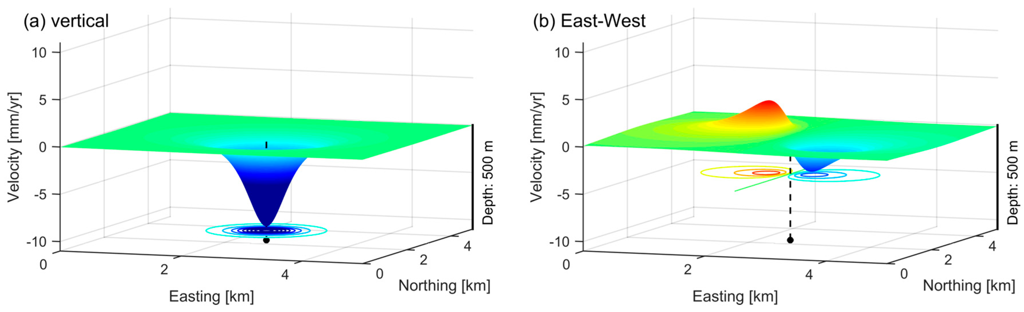
3.1. Simulated Deformation Using a Mogi Model

The Mogi model was originally developed to describe deformation occurring beneath volcanoes [63], but it is suitable as a first-order approximation for many deformation phenomena [6,70,71]. The Mogi model is a simple analytical model that describes the magnitude and direction of surface displacements resulting from the volume (or pressure) change at a point singularity within a homogeneous elastic half-space. This is a gross approximation to deformation of the Earth’s crust. Nevertheless, the Mogi model has found substantial success and ongoing use in explaining the first-order effects of a large number of real-world deformation phenomena (e.g., occurring at volcanoes, or related to mining, underground nuclear tests and groundwater withdrawal) on account of its simplicity. In fact, the Mogi model is the simplest existing model of crustal deformation, with only four variable parameters. In our simulation, the Mogi model serves as a representation of three-dimensional surface motion that we use in a general comparison with observed motion (see Section 4).

Assuming a rate of volume change $\Delta V$ at depth $d$, velocities (vertical and horizontal components $v_U$ and $v_H$) at points located on a flat surface with horizontal distance $r$ to the surface projection of the source position are given by reference [72] (p. 288) and reference [73] (p. 207):

$$v_U=\frac{3\Delta Vd}{4\pi {\left(d^2+r^2\right)}^{\frac{3}{2}}}$$

(8)

$$v_H=\frac{3\Delta Vr}{4\pi {\left(d^2+r^2\right)}^{\frac{3}{2}}}$$

(9)

Note that Equations (8) and (9) also apply for a discrete volume change between two observation times, in which case a surface displacement is the outcome. Figure 2 shows an example of velocities calculated using a Mogi model with a simulated, negative rate of volume change of 10,000 m³/yr at a depth of 500 m. The resulting subsidence rate (downward motion) is strongest at the location directly above the source and decreases with distance away from that location. Maximum horizontal velocities are offset from the source location, with the offset magnitude depending on the source depth. In this example the maximum vertical velocity is −9.55 mm/yr. The maximum horizontal velocity is ±3.68 mm/yr and located at a horizontal distance of 350 m from the source location.

Maximum vertical and horizontal velocities for varying source depths are displayed in Figure 3. A greater rate of volume change results in larger velocities. Furthermore, a larger velocity is observed for the same rate of volume change at shallower depths. However, the spatial extent of the deformation pattern reduces with decreasing depth. The ratio of maximum horizontal and vertical velocity is constant at a value of 0.385 for all source depths and rates of volume change (see also [72], p. 289). As an example, this means that for a maximum vertical displacement rate of −10 mm/yr, maximum horizontal displacement rates of ±3.85 mm/yr can be expected if the deformation source is Mogi-like.

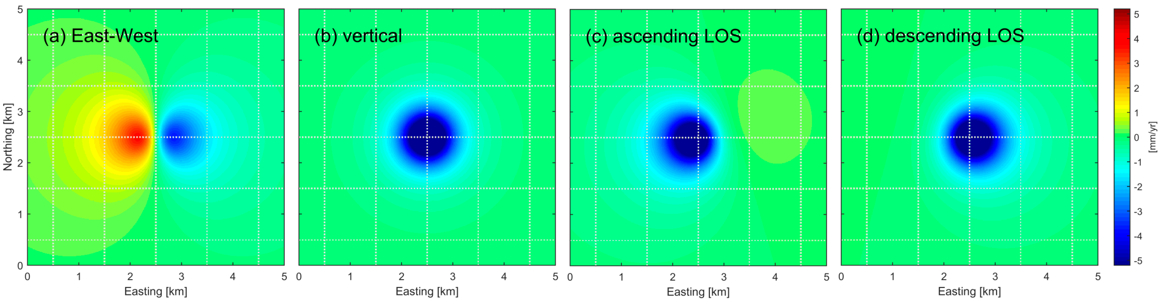
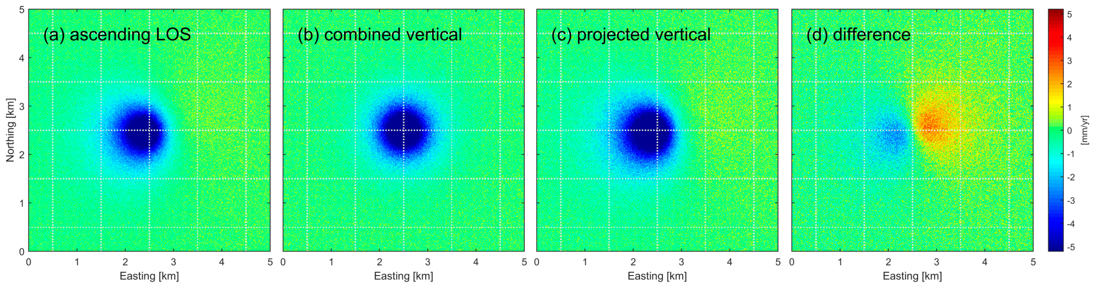
3.2. Fusion of Simulated Displacement Data

From the deformation model described in Section 3.1, we derive a 3D velocity field with signal components in the E, N and U directions. In order to simulate a multi-geometry fusion of InSAR data, we convert each 3D velocity vector $\left(\begin{array}{ccc}{v}_E& v_N& v_U\end{array}\right)$ into a LOS velocity $v_{LOS}$ using Equation (1). We consider LOS observations from different viewing geometries using the seven Envisat LOS geometries presented in Section 4. Furthermore, different levels of noise are added to the simulated LOS velocity observations by drawing random numbers from a Gaussian distribution with a defined standard deviation in order to investigate the performance of the LSA under different noise conditions. While a single InSAR interferogram usually exhibits non-Gaussian noise characteristics [74,75], spatially correlated nuisance terms are largely reduced in time series InSAR analysis (e.g., by spatio-temporal filtering of atmospheric effects). Therefore it can be shown that the resulting set of LOS velocity observations are usually close to a Gaussian distribution ([76] or [77], p. 141). Figure 4 displays the E and U components of the simulated velocity field along with the resulting velocity fields for one ascending and one descending Envisat LOS geometry. The descending geometry has a steeper incidence angle and is hence more similar to the vertical velocity field. A lateral shift of the maximum LOS velocity from the centre (where the maximum vertical velocity resides) is visible in both ascending and descending LOS velocity fields.

Comparing the vertical signal component derived from projection of LOS to vertical to the original simulated vertical signal component reveals errors with a magnitude that depends on the incidence angle and the amount of horizontal deformation.

Table 1. Mean absolute difference (MAD) and maximum difference (MAX) between projected vertical velocities and simulated velocities (both without adding noise) for different incidence angles. The maximum vertical velocity of this simulation is −9.55 mm/yr.

Incidence Angle	MAD (mm/yr)	MAX (mm/yr)
15°	0.15	0.98
20°	0.20	1.34
25°	0.26	1.71
30°	0.32	2.12
35°	0.38	2.57
40°	0.46	3.08
45°	0.55	3.68
50°	0.65	4.38

lists the mean absolute difference (MAD) and maximum difference (MAX) for different incidence angles for the simulated Mogi velocity field (Figure 4).

From Equation (1) we can mathematically derive the maximum error in the projected vertical component $\Delta {\mathrm{v}}_{\mathrm{U},\mathrm{proj},\max }$ (the maximum difference between the projected vertical to the original simulated vertical signal component; see Appendix A for a full derivation):

$$\Delta v_{U,proj,max}=v_{H,max}·tan\theta$$

(10)

where $v_{H,max}$ represents the maximum horizontal deformation (in the look direction of the sensor if the horizontal deformation is not symmetrical; see also reference [78]). This error is consistent with the numbers in Table 1 resulting from our simulation. For a Mogi-like deformation phenomenon, Equation (10) results in $0.385·tan\theta$ of the maximum vertical velocity or displacement. For example, an incidence angle of 38° and a maximum vertical displacement of 10 mm results in a maximum difference of 3 mm. Consequently, large errors are introduced when projecting LOS measurements to vertical by neglecting the horizontal component of the signal, particularly for viewing geometries with a shallow incidence angle ($\theta >30$°).

Now we combine the simulated LOS velocities using LSA as described in Section 2 to solve for 3D velocities. For the simulated LOS velocities with added random Gaussian noise, the LSA is repeated 1000 times (each with a different realisation of random noise) in order to derive statistically valid results. Furthermore, we use different combinations of available velocity observations (i.e., two, four and seven different LOS viewing geometries) to estimate velocity components in E, N and U directions or, when omitting the N component, in the E and U directions only. Figure 5 displays an example of a LOS velocity field with the addition of spatially un-correlated Gaussian noise (sigma: 0.5 mm/yr) along with the resulting vertical velocities derived from combining seven viewing geometries. For comparison, the projection of the LOS to vertical (by neglecting the horizontal signal component) and the residuals to the combined solution are also shown in Figure 5. From Figure 5d it becomes obvious that large errors are introduced to the vertical velocities when only a projection is used instead of rigorous data fusion. In our example the maximum difference between the two solutions are around 5 mm/yr, which is more than 50% of the maximum vertical velocity (around −11 mm/yr after noise has been added to the simulated observations).

When comparing the 3D velocities resulting from multi-geometry data fusion to the original velocity field derived from the Mogi deformation model, we find that without the presence of noise in the observations, LSA delivers the exact solution of the simulated input data when all three velocity components are estimated (see Figure 6a at zero noise level). However, if only the E and U components are estimated, a slight error is introduced which is greatest at locations where the surface velocities are mainly N–S directed (maximum difference of 0.7 mm/yr in the simulation with two tracks only for the U component, MAD: 0.1 mm/yr). This error is the result of neglecting the N–S component of deformation, but is acceptable in many cases with regards to the general noise level of InSAR measurements. However, for non-isotropic deformation phenomena, such as earthquakes or landslides, where the N–S component of deformation can be significantly larger than the E–W component, neglecting the N component may result in much larger errors compared to this simulation. The MAD of the estimated E, N and U velocities with respect to the model are shown in Figure 6 for the two cases when estimating all three components and when estimating only the E and U components. Using more viewing geometries in the data fusion results in lower MAD values. A linear increase of MAD values is observed when the noise level of the velocity observations increases. MAD and MAX values are summarised in

Table 2. Difference of estimated velocities to original model values for Gaussian noise level of 0.5 mm/yr, mean absolute difference (MAD) and maximum difference (MAX).

Type of Fusion	E (mm/yr)		N (mm/yr)		U (mm/yr)
	MAD	MAX	MAD	MAX	MAD	MAX
all three components
Seven tracks	0.37	2.12	3.21	18.41	0.48	2.73
Four tracks	0.45	2.61	4.60	26.32	0.63	3.63
Two tracks	-	-	-	-	-	-
E and U only
Seven tracks	0.33	1.84	-	-	0.20	1.23
Four tracks	0.45	2.51	-	-	0.24	1.43
Two tracks	0.53	3.02	-	-	0.36	2.14

for the Gaussian noise level of 0.5 mm/yr, which represents a typical noise level for C-band InSAR-derived velocities [62]. The MAD and MAX values of the N component are around a factor of 10 worse compared to the corresponding values of E and U components. From Figure 6 and Table 2 it also becomes obvious that in the presence of spatially un-correlated noise, it is better to omit the N velocity component and solve only for the E and U components of velocity when combining LOS velocities from three or more InSAR viewing geometries. In particular, the U component benefits from omitting the N component from the LSA, as evidenced by the fact that MAD and MAX values are better than a factor of two smaller (see Table 2).

4. Application to Observed Data

Within this section, we present the results of multi-geometry data fusion of InSAR-derived velocity observations from Envisat SAR data. We also compare the estimates of vertical velocities resulting from multi-geometry data fusion to those obtained by projecting the InSAR LOS to vertical and neglecting horizontal surface motions.

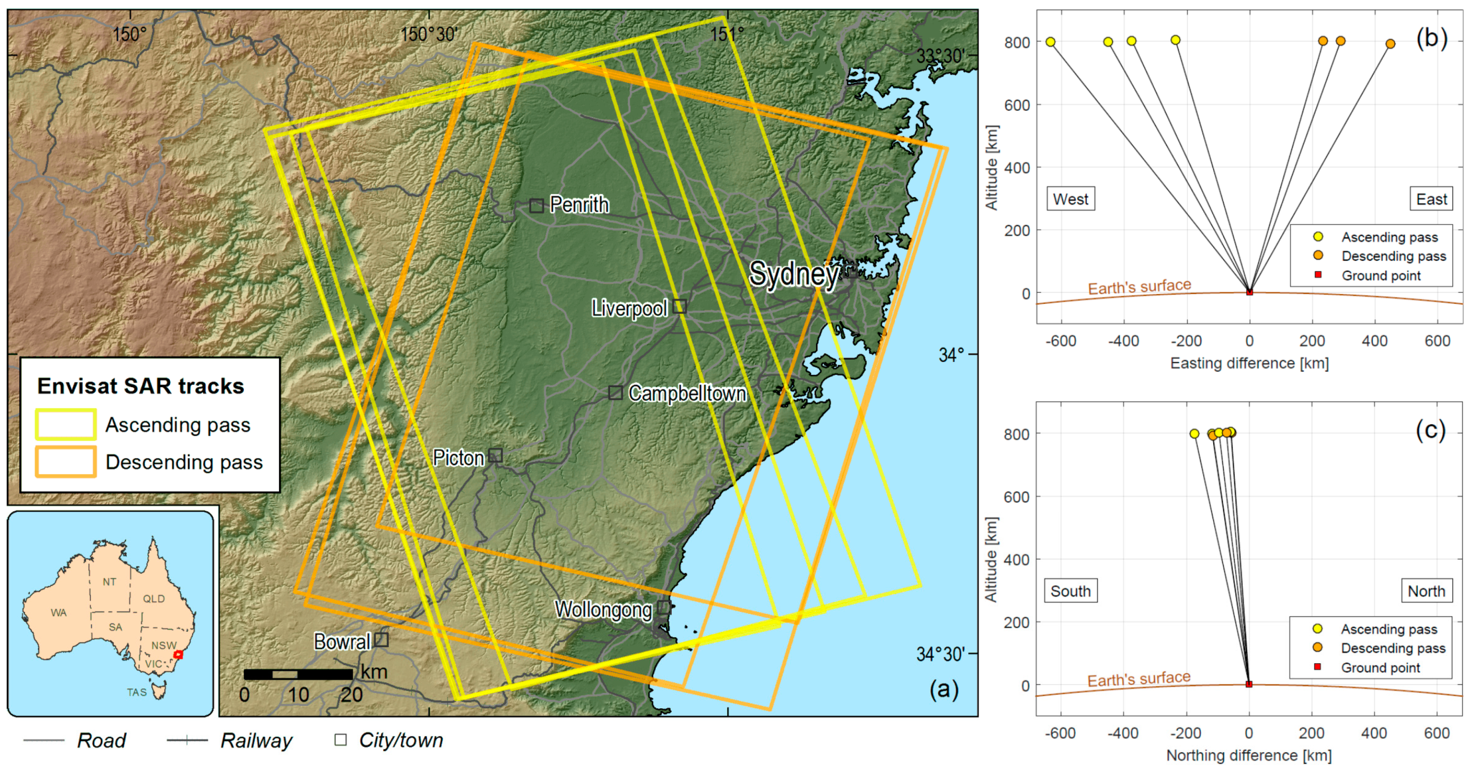
4.1. Envisat SAR Database in the Sydney Region

We use Envisat SAR data acquired in the Sydney region, on the east coast of Australia, between June 2006 and September 2010. This database is particularly suitable for an investigation of multi-geometry data fusion because a large number of images were acquired covering a similar ground area from four ascending and three descending orbital tracks (see Figure 7 and

Table 3. Overview of the seven Envisat data sets including information on the LOS geometries. A: ascending, D: descending.

Orbital Track	Pass Direction	Start Date	End Date	Number of Images Used	Number of Interferograms	Satellite Heading	Incidence Angle	Envisat Image Mode
338	A	15 June 2006	2 September 2010	42	109	−14.5°	19.0°	IS1
381	A	18 June 2006	5 September 2010	43	117	−15.5°	28.9°	IS3
152	A	2 June 2006	24 September 2010	36	97	−16.0°	33.9°	IS4
467	A	31 March 2007	31 October 2009	26	83	−17.3°	44.1°	IS7
173	D	8 July 2006	25 September 2010	31	81	−165.5°	18.9°	IS1
402	D	19 June 2006	6 September 2010	42	130	−165.1°	22.9°	IS2
359	D	16 June 2006	3 September 2010	41	129	−164.1°	33.8°	IS4

). From the different viewing geometry of each track, the pixels on the ground are observed with a different incidence angle and heading. Figure 7b,c visualise the different geometries by displaying the satellite positions in orbit at the time of acquisition with respect to a common position on the ground. The satellite positions are well distributed over the sky in the E–W plane (see Figure 7b). Multi-geometry data fusion is hence able to estimate E and U velocities when mathematically combining the LOS velocities from all seven viewing geometries. However, the variation of satellite positions in N–S plane is small (Figure 7c), meaning that any N–S directed motion will be poorly constrained even if a pixel on the ground is observed from all seven viewing geometries (cf. Equation (5)). Note that the situation shown in Figure 7 is similar for all space-borne SAR sensors since all past and current missions have a sun-synchronous low polar orbit. However, in most cases less data from different viewing geometries is available. The geometry slightly improves when data from both right- and left-looking geometries are available, which is a feature of some SAR sensors (ALOS-2, RADARSAT-2 and TerraSAR-X). However, the N–S signal component is still a factor of 4–5 worse compared to the E–W and vertical components [39,79].

Detailed information on the image acquisitions and properties of all seven Envisat viewing geometries are given in Table 3. Except for track 467, all tracks cover a similar time period of more than four years with image acquisitions regularly distributed over time (the minimum repeat time for Envisat was 35 days). Generally, more than 20 images are required to achieve high quality InSAR results [80]. The Envisat data sets in the seven viewing geometries contain between 26 and 43 usable images, which allows for a high quality InSAR analysis.

We apply the following processing strategy consistently and independently to all seven Envisat data sets:

• Calculation of a small baseline subset (SBAS) network of interferograms using the GAMMA software [81]. The SBAS network is generated based on coherence and the requirement for a minimum and maximum number of connections for each image. The results of this step are interferometric phase images with major orbital and topographic contributions to the phase signal removed.
• Time series analysis of interferometric phase using the SBAS approach [82] as implemented in the StaMPS software [83,84,85]. The results of this step are LOS displacement time series at a subset of image pixels with slowly-decorrelating phase observations.
• Quality check and outlier filtering of the resulting subset of image pixels, including the exclusion of pixels with phase unwrapping errors. Furthermore, a stable area (zero-mean and low variation of displacement values), common to all seven independent InSAR analyses is defined. The stable area then serves as a spatial reference for all InSAR-derived data sets.
• Interpolation of the LOS displacements at each measurement epoch to a regular 100 m grid (no interpolation is performed at grid nodes where no InSAR pixels are in the vicinity) and calculation of a linear displacement rate (velocity). This step is described in detail by references [62,77].

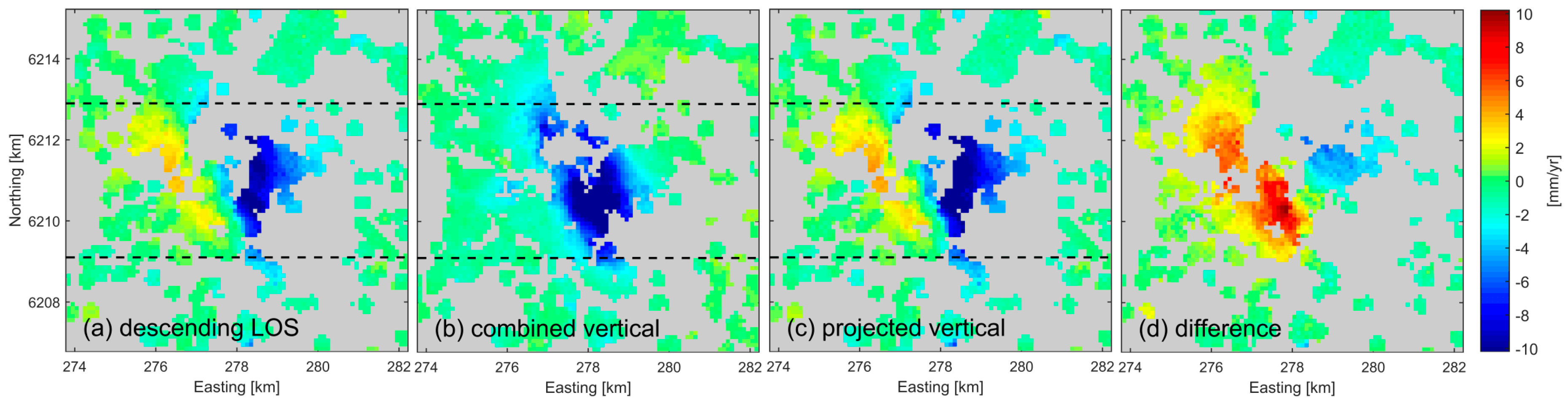
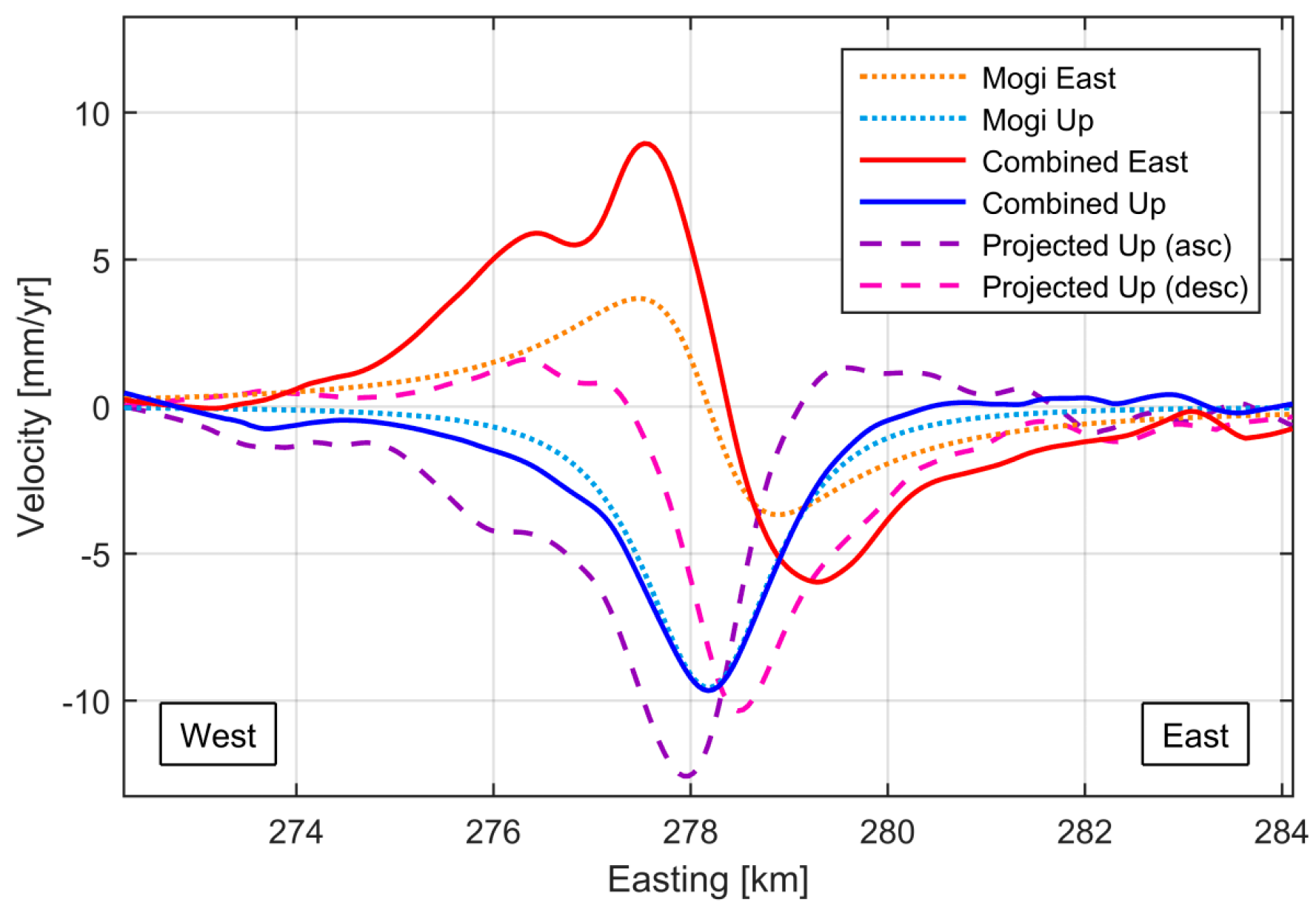
4.2. Fusion of Envisat Velocity Data

We combine the LOS velocities derived from the seven Envisat InSAR analyses by applying LSA at every interpolated grid node where there are at least three observations (for a particular grid node a LOS velocity is available from at least one ascending plus two descending geometries, or two descending plus one ascending geometries). As we demonstrated in Section 3.2, the estimated E and U velocities become more accurate when the N component is omitted from the LSA by discarding the second row of the design matrix in Equation (3). This is only valid for isotropic deformation phenomena where the N component is of the same order of magnitude as the E component. The N component should not be neglected if it is expected to be significantly greater than the E component (in the case of earthquake and landslide deformation).

Figure 8 shows the LOS velocities for one ascending and one descending geometry along with the derived E and U components derived by data fusion of the seven Envisat data sets. The northern part of the investigated area is stable, with velocities within a few millimetres per year. However, velocities of 10 mm/yr (or more) are observed in several locations in the southern part of the analysed area. Two localised patterns of surface motion can be clearly distinguished; the first southwest of Picton and the second east of Picton. In both cases, a different motion behaviour is revealed by the ascending and descending geometry. The ascending LOS velocities show negative values in the western part of the patterns and positive values in the eastern parts. The descending LOS velocities behave in the opposite fashion. These observations from different viewing geometries indicate the presence of horizontal motions in these locations. Multi-geometry data fusion of all seven data sets allows us to unravel and better understand the E and U components of these motion patterns. The E component of velocity (Figure 8c) displays the behaviour of a subsidence bowl (cf. Figure 2b and Figure 4a), with east-directed motion on the western side of the subsidence zone and west-directed motion in the eastern part. The U component reveals subsidence in both locations. In contrast to the ratio of vertical to horizontal velocities resulting from a Mogi model, the horizontal velocity field has a similar magnitude as the vertical velocity field. This indicates that the source of deformation that is causing the surface motion in these cases differs from the Mogi deformation model.

We now further investigate the deforming zone southwest of Picton. Figure 9 shows a close-up view of the descending LOS velocity field (Figure 8b), the U component derived by data fusion (Figure 8d) and the U component derived by projecting LOS to vertical (and neglecting horizontal signal components). Furthermore, we show the difference between the two derivations of the vertical velocity field (Figure 9d). The projected vertical velocities deviate from the combined vertical velocities derived from data fusion, similarly to the simulated results shown in Figure 5. However, because of the larger ratio of horizontal surface motion to vertical surface motion, the differences are larger than the simulation. In fact, the results of projecting LOS to vertical would erroneously indicate that surface uplift is occurring in the area with a velocity of up to 4.8 mm/yr (Figure 9c). The pixel-wise differences between projected vertical and combined vertical (shown in Figure 9d) range between −6.2 mm/yr and +10.2 mm/yr, which is up to 67% of the maximum absolute combined velocity (−15.2 mm/yr).

To further illustrate the implications for interpreting 3D surface motions from InSAR-derived measurements, in Figure 10 we show E–W profiles of the combined and projected velocities crossing the deforming zone shown in Figure 9. Furthermore, we compute (and show in Figure 10) a Mogi simulation that produces E and U velocities broadly matching the velocities observed in the Envisat data. The vertical velocities simulated by the Mogi model provide a good fit to the combined vertical velocity estimate, indicating that the chosen depth (500 m) and volume change rate (10,000 m³/yr) of the model are applicable to this deforming zone. However, as previously discussed, the horizontal velocities produced by this real-world deformation phenomenon exceed those of the Mogi model. This indicates that in this case the deformation source cannot be described by a single point source within an elastic half-space. Both projected U components (ascending and descending) can be seen to deviate significantly from the combined vertical and modelled vertical components. The maximum subsidence values of both projections exceed the combined ones and are shifted by several hundred metres to the west (ascending) or to the east (descending). The ascending track displayed in Figure 10 (track 467) has a relatively shallow incidence angle ($\theta =44$°), which further compounds the error effect on the projected vertical component (when compared to the descending track 359, with a steeper incidence angle, $\theta =34$°). Both ascending and descending projected U velocity estimates indicate uplift (ascending: east of the subsidence bowl, descending: west of the subsidence bowl), whereas the combined U component as well as the Mogi model indicate only subsidence. This example from a real-world data set demonstrates that projecting LOS measurements to vertical may result in misleading interpretation of InSAR-derived motions, particularly when a strong horizontal signal component is present.

5. Discussion

In Section 3 and Section 4 we have shown that projecting InSAR LOS measurements to the vertical direction whilst neglecting horizontal motion can ultimately lead to erroneous interpretation of InSAR results. Our investigations are based on velocities since these are mostly used to describe slow motion events measured with InSAR, but all results and conclusions are equally applicable to the case of displacement data. Deformation of the Earth’s crust results in surface displacements in three dimensions. The assumption of a purely vertical motion behaviour is usually only valid for a certain part of the deforming area (the central part of a subsidence bowl). Many natural and anthropogenic deformation phenomena follow a Mogi-like behaviour (to first order), which means that the maximum horizontal surface motion is around 38.5% of the maximum vertical surface motion. When projecting LOS measurements to the vertical direction by assuming there is no (or negligible) horizontal motion, an error is introduced with a magnitude that depends on the incidence angle and on the amount of horizontal motion. For an incidence angle of 26.5°, the error is 50% of the maximum horizontal motion, for an incidence angle of 45°, the error is 100% of the maximum horizontal motion. We therefore recommend not to project LOS measurements to vertical if only one image geometry is available, particularly if the incidence angle is shallow (above 30°). Instead the InSAR measurements should be interpreted in the LOS geometry, with the implications of the 1D viewing geometry clearly explained to stakeholders. When a projection of LOS to vertical is absolutely required, the maximum theoretical error can be calculated from Equation (10). This results in $0.385·tan\theta$ of the maximum vertical motion for a Mogi deformation source. However, depending on the deformation phenomenon, we find that this error can be much larger in the real world. For surface motions observed in the Sydney region in Envisat SAR data, an error of up to 67% of the maximum vertical motion is introduced when projecting LOS measurements at an incidence angle of 33.8°. Apart from incorrect magnitude and direction of resulting vertical surface motions (uplift instead of subsidence in some parts of the deformation field), the location of the maximum vertical motion was found (in the case of the deforming zone southwest of Picton) to be shifted by several hundred metres. These implications could lead to incorrect validation of InSAR observations with those derived from GNSS or other geodetic techniques, and ultimately may lead to a lack of trust in the InSAR technique. Instead of comparing a projected vertical InSAR displacement to the vertical GNSS component [30], we recommend transforming the 3D GNSS measurements into the corresponding InSAR LOS geometry for validation purposes [86].

If InSAR data is available on multiple tracks for the same area of interest, multi-geometry data fusion is the best way to gain insight into the 3D surface behaviour of subsurface deformation processes. Spatial interpolation is needed to provide LOS measurements from InSAR analysis of several viewing geometries at the same locations. Rigorous results of combined E–W and vertical motion estimates are then derived from LSA of LOS measurements and their uncertainties derived from single-geometry InSAR analysis. For the case of LOS measurements being available in three or more viewing geometries, we find that it is better to omit the N–S component from the LSA, as the poor condition of the design matrix introduces errors into the estimated parameters, particularly the vertical component. The usage of exact incidence angles for each grid pixel in the design matrix shown in Equation (3) becomes particularly important when combining Interferometric Wide Swath data from the European Space Agency’s Sentinel-1 mission [87] because of the large variation of the incidence angle from near-range to far-range. Sentinel-1 InSAR measurements are particularly suited to multi-geometry data fusion, since for many regions on Earth, data are available from both ascending and descending orbital passes and with a large overlap of images acquired from adjacent orbital tracks.

The approach we have described in this paper can also be used with input data from different SAR sensors, and measured over different time periods. Note that interpolation in time and fusion of displacements at different time steps (instead of velocities) is needed if the deformation is non-linear. Furthermore, the matrix notation used in the LSA can be extended to add in other geodetic data such as levelling or GNSS measurements [61,62]. In addition, surface motions derived from GNSS data are particularly valuable for validation of large-scale InSAR products and for incorporation of relative InSAR measurements derived on numerous adjacent orbital tracks into seamless mosaicked products [88,89,90,91] that can be used to add a much higher density of geodetic measurements to national geodetic products such as a height datum [86].

6. Conclusions

In this paper we have investigated the implications of the InSAR LOS geometry for measuring 3D surface motions. We have compared the results of multi-geometry InSAR data fusion of simulated and observed LOS velocities to the results of projecting LOS velocities to vertical (by neglecting the presence of horizontal motions). This comparison has demonstrated the advantages of fusing LOS measurements from several different viewing geometries. With regards to the research questions defined in Section 1, we give the following conclusions and recommendations:

• Projection of InSAR LOS measurements into the vertical direction without considering the impact of horizontal motion is generally not recommended. Instead, data from ascending and descending geometries should be combined whenever available in the area of interest. The error in the projected vertical measurement depends on the amount of horizontal motion as well as on the incidence angle $\theta$ of the LOS geometry. As a rule of thumb (assuming Mogi-like deformation), the maximum error introduced into the projected vertical measurement can be approximated by $0.385·tan\theta$ of the maximum vertical motion. Vertical measurements resulting from LOS projection can be wrong in terms of magnitude, direction and location.
• Multi-geometry data fusion of LOS InSAR measurements from several viewing geometries allows for robust estimation of horizontal and vertical motions. Weighted LSA can be applied when data from three or more viewing geometries are available with at least one ascending and one descending geometry. The matrix formulation for data fusion on a pixel-by-pixel basis allows for inclusion of data from different sensors (X-band, C-band, L-band, etc.) as well as independent data sources such as GNSS. Using exact incidence angles for each pixel is recommended, since large variations of incidence angle across range exist for most InSAR imaging geometries (17° over the full 250 km extent of a Sentinel-1 Interferometric Wide Swath image).
• The N–S component of motion resulting from multi-geometry data fusion of LOS InSAR measurements derived from past or current space-borne SAR sensors is poorly constrained, even if several different geometries are available (InSAR data from seven different tracks). If the N–S component is expected to be at a similar magnitude as the E–W component or smaller, less error is introduced into the combined results by omitting the N–S component from the LSA and only solving for the vertical and E–W components of motion.

References

1. Ferretti, A.; Prati, C.; Rocca, F. Nonlinear subsidence rate estimation using permanent scatterers in differential SAR interferometry. IEEE Trans. Geosci. Remote Sens. 2000, 38, 2202–2212. [Google Scholar] [CrossRef]
2. Ferretti, A.; Prati, C.; Rocca, F. Permanent scatterers in SAR interferometry. IEEE Trans. Geosci. Remote Sens. 2001, 39, 8–20. [Google Scholar] [CrossRef] [Green Version]
3. Adam, N.; Kampes, B.; Eineder, M.; Worawattanamateekul, J.; Kircher, M. The development of a scientific permanent scatterer system. In Proceedings of the ISPRS Workshop High Resolution Mapping from Space, Hannover, Germany, 23–25 December 2003. [Google Scholar]
4. Hooper, A.; Zebker, H.; Segall, P.; Kampes, B. A new method for measuring deformation on volcanoes and other natural terrains using InSAR persistent scatterers. Geophys. Res. Lett. 2004, 31. [Google Scholar] [CrossRef] [Green Version]
5. Kampes, B.M. Displacement Parameter Estimation Using Permanent Scatterer Interferometry. Ph.D. Thesis, Delft University of Technology, Delft, The Netherlands, 2005. [Google Scholar]
6. Hanssen, R.F. Radar Interferometry: Data Interpretation and Error Analysis; Kluwer Academic Publishers: Dordrecht, The Netherlands, 2001. [Google Scholar]
7. Teatini, P.; Tosi, L.; Strozzi, T.; Carbognin, L.; Wegmüller, U.; Rizzetto, F. Mapping regional land displacements in the Venice coastland by an integrated monitoring system. Remote Sens. Environ. 2005, 98, 403–413. [Google Scholar] [CrossRef]
8. Stramondo, S.; Bozzano, F.; Marra, F.; Wegmuller, U.; Cinti, F.R.; Moro, M.; Saroli, M. Subsidence induced by urbanisation in the city of Rome detected by advanced InSAR technique and geotechnical investigations. Remote Sens. Environ. 2008, 112, 3160–3172. [Google Scholar] [CrossRef]
9. Solari, L.; Ciampalini, A.; Raspini, F.; Bianchini, S.; Moretti, S. PSInSAR Analysis in the Pisa Urban Area (Italy): A Case Study of Subsidence Related to Stratigraphical Factors and Urbanization. Remote Sens. 2016, 8, 120. [Google Scholar] [CrossRef]
10. Yang, C.-S.; Zhang, Q.; Xu, Q.; Zhao, C.-Y.; Peng, J.-B.; Ji, L.-Y. Complex Deformation Monitoring over the Linfen–Yuncheng Basin (China) with Time Series InSAR Technology. Remote Sens. 2016, 8, 284. [Google Scholar] [CrossRef]
11. Zhou, L.; Guo, J.; Hu, J.; Li, J.; Xu, Y.; Pan, Y.; Shi, M. Wuhan Surface Subsidence Analysis in 2015–2016 Based on Sentinel-1A Data by SBAS-InSAR. Remote Sens. 2017, 9, 982. [Google Scholar] [CrossRef]
12. Zheng, M.; Deng, K.; Fan, H.; Du, S. Monitoring and Analysis of Surface Deformation in Mining Area Based on InSAR and GRACE. Remote Sens. 2018, 10, 1392. [Google Scholar] [CrossRef]
13. Galloway, D.L.; Hudnut, K.W.; Ingebritsen, S.E.; Phillips, S.P.; Peltzer, G.; Rogez, F.; Rosen, P.A. Detection of aquifer system compaction and land subsidence using interferometric synthetic aperture radar, Antelope Valley, Mojave Desert, California. Water Resour. Res. 1998, 34, 2573–2585. [Google Scholar] [CrossRef] [Green Version]
14. Amelung, F.C.; Galloway, D.L.; Bell, J.W.; Zebker, H.A.; Laczniak, R.J. Sensing the ups and downs of Las Vegas. Geology 1999, 27, 483–486. [Google Scholar] [CrossRef]
15. Schmidt, D.A.; Bürgmann, R. Time-dependent land uplift and subsidence in the Santa Clara valley, California, from a large interferometric synthetic aperture radar data set. J. Geophys. Res. Solid Earth 2003, 108. [Google Scholar] [CrossRef] [Green Version]
16. Wisely, B.A.; Schmidt, D. Deciphering vertical deformation and poroelastic parameters in a tectonically active fault-bound aquifer using InSAR and well level data, San Bernardino basin, California. Geophys. J. Int. 2010, 181, 1185–1200. [Google Scholar] [CrossRef] [Green Version]
17. Hung, W.-C.; Hwang, C.; Chen, Y.-A.; Chang, C.-P.; Yen, J.-Y.; Hooper, A.; Yang, C.-Y. Surface deformation from persistent scatterers SAR interferometry and fusion with leveling data: A case study over the Choushui River Alluvial Fan, Taiwan. Remote Sens. Environ. 2011, 115, 957–967. [Google Scholar] [CrossRef]
18. Wang, H.; Wright, T.J.; Yu, Y.; Lin, H.; Jiang, L.; Li, C.; Qiu, G. InSAR reveals coastal subsidence in the Pearl River Delta, China. Geophys. J. Int. 2012, 191, 1119–1128. [Google Scholar] [CrossRef]
19. Chaussard, E.; Amelung, F.; Abidin, H.; Hong, S.-H. Sinking cities in Indonesia: ALOS PALSAR detects rapid subsidence due to groundwater and gas extraction. Remote Sens. Environ. 2013, 128, 150–161. [Google Scholar] [CrossRef]
20. Ge, L.; Ng, A.H.-M.; Li, X.; Abidin, H.Z.; Gumilar, I. Land subsidence characteristics of Bandung Basin as revealed by ENVISAT ASAR and ALOS PALSAR interferometry. Remote Sens. Environ. 2014, 154, 46–60. [Google Scholar] [CrossRef]
21. Qu, F.; Lu, Z.; Zhang, Q.; Bawden, G.W.; Kim, J.-W.; Zhao, C.; Qu, W. Mapping ground deformation over Houston-Galveston, Texas using multi-temporal InSAR. Remote Sens. Environ. 2015, 169, 290–306. [Google Scholar] [CrossRef]
22. Du, Z.; Ge, L.; Li, X.; Ng, A. Subsidence Monitoring over the Southern Coalfield, Australia Using both L-Band and C-Band SAR Time Series Analysis. Remote Sens. 2016, 8, 543. [Google Scholar] [CrossRef]
23. Xu, B.; Feng, G.; Li, Z.; Wang, Q.; Wang, C.; Xie, R. Coastal Subsidence Monitoring Associated with Land Reclamation Using the Point Target Based SBAS-InSAR Method: A Case Study of Shenzhen, China. Remote Sens. 2016, 8, 652. [Google Scholar] [CrossRef]
24. Zhang, Y.; Wu, H.a.; Kang, Y.; Zhu, C. Ground Subsidence in the Beijing-Tianjin-Hebei Region from 1992 to 2014 Revealed by Multiple SAR Stacks. Remote Sens. 2016, 8, 675. [Google Scholar] [CrossRef]
25. Parker, A.; Filmer, M.; Featherstone, W. First Results from Sentinel-1A InSAR over Australia: Application to the Perth Basin. Remote Sens. 2017, 9, 299. [Google Scholar] [CrossRef]
26. Alshammari, L.; Large, D.; Boyd, D.; Sowter, A.; Anderson, R.; Andersen, R.; Marsh, S. Long-Term Peatland Condition Assessment via Surface Motion Monitoring Using the ISBAS DInSAR Technique over the Flow Country, Scotland. Remote Sens. 2018, 10, 1103. [Google Scholar] [CrossRef]
27. Gao, M.; Gong, H.; Chen, B.; Li, X.; Zhou, C.; Shi, M.; Si, Y.; Chen, Z.; Duan, G. Regional Land Subsidence Analysis in Eastern Beijing Plain by InSAR Time Series and Wavelet Transforms. Remote Sens. 2018, 10, 365. [Google Scholar] [CrossRef]
28. Hung, W.-C.; Hwang, C.; Chen, Y.-A.; Zhang, L.; Chen, K.-H.; Wei, S.-H.; Huang, D.-R.; Lin, S.-H. Land Subsidence in Chiayi, Taiwan, from Compaction Well, Leveling and ALOS/PALSAR: Aquaculture-Induced Relative Sea Level Rise. Remote Sens. 2018, 10, 40. [Google Scholar] [CrossRef]
29. Ng, A.; Wang, H.; Dai, Y.; Pagli, C.; Chen, W.; Ge, L.; Du, Z.; Zhang, K. InSAR Reveals Land Deformation at Guangzhou and Foshan, China between 2011 and 2017 with COSMO-SkyMed Data. Remote Sens. 2018, 10, 813. [Google Scholar] [CrossRef]
30. Tang, W.; Yuan, P.; Liao, M.; Balz, T. Investigation of Ground Deformation in Taiyuan Basin, China from 2003 to 2010, with Atmosphere-Corrected Time Series InSAR. Remote Sens. 2018, 10, 1499. [Google Scholar] [CrossRef]
31. Yang, M.; Yang, T.; Zhang, L.; Lin, J.; Qin, X.; Liao, M. Spatio-Temporal Characterization of a Reclamation Settlement in the Shanghai Coastal Area with Time Series Analyses of X-, C-, and L-Band SAR Datasets. Remote Sens. 2018, 10, 329. [Google Scholar] [CrossRef]
32. Raucoules, D.; Maisons, C.; Carnec, C.; Le Mouelic, S.; King, C.; Hosford, S. Monitoring of slow ground deformation by ERS radar interferometry on the Vauvert salt mine (France): Comparison with ground-based measurement. Remote Sens. Environ. 2003, 88, 468–478. [Google Scholar] [CrossRef]
33. Short, N.; LeBlanc, A.-M.; Sladen, W.; Oldenborger, G.; Mathon-Dufour, V.; Brisco, B. RADARSAT-2 D-InSAR for ground displacement in permafrost terrain, validation from Iqaluit Airport, Baffin Island, Canada. Remote Sens. Environ. 2014, 141, 40–51. [Google Scholar] [CrossRef]
34. Sun, H.; Zhang, Q.; Zhao, C.; Yang, C.; Sun, Q.; Chen, W. Monitoring land subsidence in the southern part of the lower Liaohe plain, China with a multi-track PS-InSAR technique. Remote Sens. Environ. 2017, 188, 73–84. [Google Scholar] [CrossRef]
35. Zhou, W.; Li, S.; Zhou, Z.; Chang, X. Remote Sensing of Deformation of a High Concrete-Faced Rockfill Dam Using InSAR: A Study of the Shuibuya Dam, China. Remote Sens. 2016, 8, 255. [Google Scholar] [CrossRef]
36. Zhou, C.; Gong, H.; Chen, B.; Li, J.; Gao, M.; Zhu, F.; Chen, W.; Liang, Y. InSAR Time-Series Analysis of Land Subsidence under Different Land Use Types in the Eastern Beijing Plain, China. Remote Sens. 2017, 9, 380. [Google Scholar] [CrossRef]
37. Chen, G.; Zhang, Y.; Zeng, R.; Yang, Z.; Chen, X.; Zhao, F.; Meng, X. Detection of Land Subsidence Associated with Land Creation and Rapid Urbanization in the Chinese Loess Plateau Using Time Series InSAR: A Case Study of Lanzhou New District. Remote Sens. 2018, 10, 270. [Google Scholar] [CrossRef]
38. Milillo, P.; Giardina, G.; DeJong, M.; Perissin, D.; Milillo, G. Multi-Temporal InSAR Structural Damage Assessment: The London Crossrail Case Study. Remote Sens. 2018, 10, 287. [Google Scholar] [CrossRef]
39. Wright, T.J.; Parsons, B.E.; Lu, Z. Toward mapping surface deformation in three dimensions using InSAR. Geophys. Res. Lett. 2004, 31. [Google Scholar] [CrossRef] [Green Version]
40. Teatini, P.; Castelletto, N.; Ferronato, M.; Gambolati, G.; Janna, C.; Cairo, E.; Marzorati, D.; Colombo, D.; Ferretti, A.; Bagliani, A.; et al. Geomechanical response to seasonal gas storage in depleted reservoirs: A case study in the Po River basin, Italy. J. Geophys. Res. Earth Surf. 2011, 116. [Google Scholar] [CrossRef] [Green Version]
41. Ferretti, A. Satellite InSAR data: Reservoir Monitoring from Space; EAGE Publications: Houten, The Netherlands, 2014. [Google Scholar]
42. Lundgren, P.; Casu, F.; Manzo, M.; Pepe, A.; Berardino, P.; Sansosti, E.; Lanari, R. Gravity and magma induced spreading of Mount Etna volcano revealed by satellite radar interferometry. Geophys. Res. Lett. 2004, 31. [Google Scholar] [CrossRef] [Green Version]
43. Borgia, A.; Tizzani, P.; Solaro, G.; Manzo, M.; Casu, F.; Luongo, G.; Pepe, A.; Berardino, P.; Fornaro, G.; Sansosti, E.; et al. Volcanic spreading of Vesuvius, a new paradigm for interpreting its volcanic activity. Geophys. Res. Lett. 2005, 32. [Google Scholar] [CrossRef] [Green Version]
44. Manzo, M.; Ricciardi, G.P.; Casu, F.; Ventura, G.; Zeni, G.; Borgström, S.; Berardino, P.; Del Gaudio, C.; Lanari, R. Surface deformation analysis in the Ischia Island (Italy) based on spaceborne radar interferometry. J. Volcanol. Geotherm. Res. 2006, 151, 399–416. [Google Scholar] [CrossRef]
45. Lanari, R.; Casu, F.; Manzo, M.; Zeni, G.; Berardino, P.; Manunta, M.; Pepe, A. An Overview of the Small BAseline Subset Algorithm: A DInSAR Technique for Surface Deformation Analysis. In Deformation and Gravity Change: Indicators of Isostasy, Tectonics, Volcanism, and Climate Change; Birkhäuser: Basel, Switherlands, 2007; pp. 637–661. [Google Scholar]
46. Fialko, Y.; Simons, M.; Agnew, D. The complete (3-D) surface displacement field in the epicentral area of the 1999 MW7.1 Hector Mine Earthquake, California, from space geodetic observations. Geophys. Res. Lett. 2001, 28, 3063–3066. [Google Scholar] [CrossRef]
47. de Michele, M.; Raucoules, D.; de Sigoyer, J.; Pubellier, M.; Chamot-Rooke, N. Three-dimensional surface displacement of the 2008 May 12 Sichuan earthquake (China) derived from Synthetic Aperture Radar: Evidence for rupture on a blind thrust. Geophys. J. Int. 2010, 183, 1097–1103. [Google Scholar] [CrossRef]
48. Raucoules, D.; de Michele, M.; Malet, J.P.; Ulrich, P. Time-variable 3D ground displacements from high-resolution synthetic aperture radar (SAR). application to La Valette landslide (South French Alps). Remote Sens. Environ. 2013, 139, 198–204. [Google Scholar] [CrossRef] [Green Version]
49. Wang, X.; Liu, G.; Yu, B.; Dai, K.; Zhang, R.; Ma, D.; Li, Z. An integrated method based on DInSAR, MAI and displacement gradient tensor for mapping the 3D coseismic deformation field related to the 2011 Tarlay earthquake (Myanmar). Remote Sens. Environ. 2015, 170, 388–404. [Google Scholar] [CrossRef]
50. Jo, M.-J.; Jung, H.-S.; Won, J.-S.; Lundgren, P. Measurement of three-dimensional surface deformation by Cosmo-SkyMed X-band radar interferometry: Application to the March 2011 Kamoamoa fissure eruption, Kīlauea Volcano, Hawai’i. Remote Sens. Environ. 2015, 169, 176–191. [Google Scholar] [CrossRef]
51. Jo, M.-J.; Jung, H.-S.; Won, J.-S. Measurement of precise three-dimensional volcanic deformations via TerraSAR-X synthetic aperture radar interferometry. Remote Sens. Environ. 2017, 192, 228–237. [Google Scholar] [CrossRef]
52. Hu, J.; Li, Z.W.; Ding, X.L.; Zhu, J.J.; Zhang, L.; Sun, Q. Resolving three-dimensional surface displacements from InSAR measurements: A review. Earth-Sci. Rev. 2014, 133, 1–17. [Google Scholar] [CrossRef]
53. Burgmann, R.; Hilley, G.; Ferretti, A.; Novali, F. Resolving vertical tectonics in the San Francisco Bay Area from permanent scatterer InSAR and GPS analysis. Geology 2006, 34, 221–224. [Google Scholar] [CrossRef]
54. Gourmelen, N.; Amelung, F.; Lanari, R. Interferometric synthetic aperture radar—GPS integration: Interseismic strain accumulation across the Hunter Mountain fault in the eastern California shear zone. J. Geophys. Res. Solid Earth 2010, 115. [Google Scholar] [CrossRef]
55. Hammond, W.C.; Blewitt, G.; Li, Z.; Plag, H.-P.; Kreemer, C. Contemporary uplift of the Sierra Nevada, western United States, from GPS and InSAR measurements. Geology 2012, 40, 667–670. [Google Scholar] [CrossRef]
56. Hussain, E.; Wright, T.J.; Walters, R.J.; Bekaert, D.P.S.; Lloyd, R.; Hooper, A. Constant strain accumulation rate between major earthquakes on the North Anatolian Fault. Nat. Commun. 2018, 9, 1392. [Google Scholar] [CrossRef] [PubMed] [Green Version]
57. Gudmundsson, S.; Gudmundsson, M.T.; Björnsson, H.; Sigmundsson, F.; Rott, H.; Carstensen, J.M. Three-dimensional glacier surface motion maps at the Gjálp eruption site, Iceland, inferred from combining InSAR and other ice-displacement data. Ann. Glaciol. 2002, 34, 315–322. [Google Scholar] [CrossRef]
58. Samsonov, S.; Tiampo, K. Analytical optimization of a DInSAR and GPS dataset for derivation of three-dimensional surface motion. IEEE Geosci. Remote Sens. Lett. 2006, 3, 107–111. [Google Scholar] [CrossRef]
59. Catalao, J.; Nico, G.; Hanssen, R.; Catita, C. Merging GPS and Atmospherically Corrected InSAR Data to Map 3-D Terrain Displacement Velocity. IEEE Trans. Geosci. Remote Sens. 2011, 49, 2354–2360. [Google Scholar] [CrossRef] [Green Version]
60. Hu, J.; Zhu, J.J.; Li, Z.W.; Ding, X.L.; Wang, C.C.; Sun, Q. Robust Estimating Three-Dimensional Ground Motions from Fusion of InSAR and GPS Measurements. In Proceedings of the 2011 International Symposium on Image and Data Fusion, Tengchong, China, 9–11 August 2011; pp. 1–4. [Google Scholar]
61. Caro Cuenca, M.; Hanssen, R.F.; Hooper, A.; Arikan, M. Surface Deformation of the Whole Netherlands After PSI Analysis. In Proceedings of the Fringe 2011 Workshop, Frascati, Italy, 19–23 September 2011; pp. 1–8. [Google Scholar]
62. Fuhrmann, T.; Caro Cuenca, M.; Knöpfler, A.; van Leijen, F.J.; Mayer, M.; Westerhaus, M.; Hanssen, R.F.; Heck, B. Estimation of small surface displacements in the Upper Rhine Graben area from a combined analysis of PS-InSAR, levelling and GNSS data. Geophys. J. Int. 2015, 203, 614–631. [Google Scholar] [CrossRef]
63. Mogi, K. Relations between the eruptions of various volcanoes and the deformations of the ground surfaces around them. Bull. Earthq. Res. Inst. 1958, 36, 99–134. [Google Scholar]
64. Van Leijen, F.J. Persistent Scatterer Interferometry Based on Geodetic Estimation Theory. Ph.D. Thesis, Delft University of Technology, Delft, The Netherlands, 2014. [Google Scholar]
65. ESA. EnviSat ASAR Product Handbook, Issue 2.2. 2007, p. 564. Available online: https://earth.esa.int/pub/ESA_DOC/ENVISAT/ASAR/asar.ProductHandbook.2_2.pdf (accessed on 24 January 2019).
66. ESA. Sentinel-1 SAR User Guide—Interferometric Wide Swath. 2018. Available online: https://sentinels.copernicus.eu/web/sentinel/user-guides/sentinel-1-sar/acquisition-modes/interferometric-wide-swath (accessed on 24 January 2019).
67. Li, J.; Heap, A.D. A Review of Spatial Interpolation Methods for Environmental Scientists; Record 2008/23 Geoscience Australia: Canberra, Australia, 2008.
68. Dai, K.; Liu, G.; Li, Z.; Li, T.; Yu, B.; Wang, X.; Singleton, A. Extracting Vertical Displacement Rates in Shanghai (China) with Multi-Platform SAR Images. Remote Sens. 2015, 7, 9542. [Google Scholar] [CrossRef]
69. Tarantola, A. Inverse Problem Theory and Methods for Model Parameter Estimation; Society for Industrial and Applied Mathematics: Philadelphia, PA, USA, 2005; p. 348. [Google Scholar]
70. Mossop, A.; Segall, P. Subsidence at The Geysers Geothermal Field, N. California from a comparison of GPS and leveling surveys. Geophys. Res. Lett. 1997, 24, 1839–1842. [Google Scholar] [CrossRef] [Green Version]
71. Carnec, C.; Fabriol, H. Monitoring and modeling land subsidence at the Cerro Prieto Geothermal Field, Baja California, Mexico, using SAR interferometry. Geophys. Res. Lett. 1999, 26, 1211–1214. [Google Scholar] [CrossRef]
72. Lisowski, M. Analytical volcano deformation source models. In Volcano Deformation: Geodetic Monitoring Techniques; Springer: Berlin/Heidelberg, Germany, 2006; pp. 279–304. [Google Scholar] [CrossRef]
73. Segall, P. Earthquake and Volcano Deformation; Princeton University Press: Princeton, NJ, USA, 2010. [Google Scholar]
74. Dawson, J.; Tregoning, P. Uncertainty analysis of earthquake source parameters determined from InSAR: A simulation study. J. Geophys. Res. Solid Earth 2007, 112. [Google Scholar] [CrossRef] [Green Version]
75. Rocca, F. Modeling Interferogram Stacks. IEEE Trans. Geosci. Remote Sens. 2007, 45, 3289–3299. [Google Scholar] [CrossRef]
76. Gourmelen, N.; Amelung, F.; Casu, F.; Manzo, M.; Lanari, R. Mining-related ground deformation in Crescent Valley, Nevada: Implications for sparse GPS networks. Geophys. Res. Lett. 2007, 34. [Google Scholar] [CrossRef] [Green Version]
77. Fuhrmann, T. Surface Displacements from Fusion of Geodetic Measurement Techniques Applied to the Upper Rhine Graben Area. Ph.D. Thesis, Karlsruhe Institute of Technology (KIT), Karlsruhe, Germany, 2016. [Google Scholar]
78. Samieie-Esfahany, S.; Hanssen, R.F.; van Thienen-Visser, K.; Muntendam-Bos, A. On the effect of horizontal deformation on InSAR subsidence estimates. In Proceedings of the Fringe 2009 Workshop, Frascati, Italy, 30 November–4 December 2009; pp. 1–7. [Google Scholar]
79. Morishita, Y.; Kobayashi, T.; Yarai, H. Three-dimensional deformation mapping of a dike intrusion event in Sakurajima in 2015 by exploiting the right- and left-looking ALOS-2 InSAR. Geophys. Res. Lett. 2016, 43, 4197–4204. [Google Scholar] [CrossRef]
80. Adam, N.; Kampes, B.; Eineder, M. Development of a Scientific Permanent Scatterer System: Modifications for Mixed ERS/ENVISAT Time Series. In Proceedings of the Envisat Symposium 2004, Salzburg, Austria, 6–10 September 2004. [Google Scholar]
81. Wegmüller, U.; Werner, C. GAMMA SAR processor and interferometry software. In Proceedings of the Third ERS Symposium on Space at the Service of Our Environment, Florence, Italy, 14–21 March 1997. [Google Scholar]
82. Berardino, P.; Fornaro, G.; Lanari, R.; Sansosti, E. A new algorithm for surface deformation monitoring based on small baseline differential SAR interferograms. IEEE Trans. Geosci. Remote Sens. 2002, 40, 2375–2383. [Google Scholar] [CrossRef]
83. Hooper, A.; Segall, P.; Zebker, H. Persistent scatterer interferometric synthetic aperture radar for crustal deformation analysis, with application to Volcán Alcedo, Galápagos. J. Geophys. Res. Solid Earth 2007, 112. [Google Scholar] [CrossRef] [Green Version]
84. Hooper, A. A multi-temporal InSAR method incorporating both persistent scatterer and small baseline approaches. Geophys. Res. Lett. 2008, 35. [Google Scholar] [CrossRef] [Green Version]
85. Hooper, A.; Bekaert, D.; Spaans, K.; Arıkan, M. Recent advances in SAR interferometry time series analysis for measuring crustal deformation. Tectonophysics 2012, 514–517, 1–13. [Google Scholar] [CrossRef]
86. Fuhrmann, T.; Garthwaite, M.; Lawrie, S.; Brown, N. Combination of GNSS and InSAR for Future Australian Datums. In Proceedings of the IGNSS Symposium 2018, Sydney, Australia, 7–9 February 2018; pp. 1–13. [Google Scholar]
87. Torres, R.; Snoeij, P.; Geudtner, D.; Bibby, D.; Davidson, M.; Attema, E.; Potin, P.; Rommen, B.; Floury, N.; Brown, M.; et al. GMES Sentinel-1 mission. Remote Sens. Environ. 2012, 120, 9–24. [Google Scholar] [CrossRef]
88. Costantini, M.; Ferretti, A.; Minati, F.; Falco, S.; Trillo, F.; Colombo, D.; Novali, F.; Malvarosa, F.; Mammone, C.; Vecchioli, F.; et al. Analysis of surface deformations over the whole Italian territory by interferometric processing of ERS, Envisat and COSMO-SkyMed radar data. Remote Sens. Environ. 2017, 202, 250–275. [Google Scholar] [CrossRef]
89. De Luca, C.; Zinno, I.; Manunta, M.; Lanari, R.; Casu, F. Large areas surface deformation analysis through a cloud computing P-SBAS approach for massive processing of DInSAR time series. Remote Sens. Environ. 2017, 202, 3–17. [Google Scholar] [CrossRef]
90. Kalia, A.C.; Frei, M.; Lege, T. A Copernicus downstream-service for the nationwide monitoring of surface displacements in Germany. Remote Sens. Environ. 2017, 202, 234–249. [Google Scholar] [CrossRef]
91. Novellino, A.; Cigna, F.; Brahmi, M.; Sowter, A.; Bateson, L.; Marsh, S. Assessing the Feasibility of a National InSAR Ground Deformation Map of Great Britain with Sentinel-1. Geosciences 2017, 7, 19. [Google Scholar] [CrossRef]
Figure 1. Schematic view of the interferometric synthetic aperture radar (InSAR) viewing geometry for line of sight (LOS) measurements on ascending and descending satellite passes.
Remotesensing 11 00241 g001
Figure 2. Simulated velocity fields resulting from a Mogi deformation source with a volume change of 10,000 m3/yr at 500 m depth: (a) vertical surface velocity (subsidence rate) resulting from a negative rate of volume change, (b) E–W component of velocity resulting from the same rate of volume change. Top-view images of (a) and (b) are displayed in Figure 4b and a, respectively.
Remotesensing 11 00241 g002
Figure 3. Maximum vertical and horizontal displacement rates resulting from Mogi model simulations with varying source depths and volume changes. Displacement rate is expressed as velocity in mm/yr assuming a steady volume change resulting in a constant displacement rate. Three discrete rates of volume change are compared for vertical and horizontal motion in (a). Contours of maximum vertical (b) and horizontal (c) velocities in mm/yr plotted as a function of depth and volume change of the source.
Remotesensing 11 00241 g003
Figure 4. Simulated velocities from a Mogi deformation model: (a) E component, (b) U component, (c) ascending LOS with −16.0° heading and 33.9° incidence angle, (d) descending LOS with −165.5° heading and 18.9° incidence angle. Note that the colour scale saturates at ±5 mm/yr. The N–S component is equivalent to the E–W component due to the symmetry of the Mogi model, but rotated anti-clockwise by 90°.
Remotesensing 11 00241 g004
Figure 5. Simulated velocities at Gaussian noise level 0.5 mm/yr (one realisation from 1000 runs): (a) ascending LOS with −16.0° heading and 33.9° incidence angle, (b) estimated U component from fusion of seven viewing geometries, (c) U component from projection of LOS velocities, (d) difference between (b) and (c). Note that the colour scale saturates at ±5 mm/yr.
Remotesensing 11 00241 g005
Figure 6. Mean absolute difference (MAD) between estimated and modelled velocity components at different noise levels and for different combinations, i.e., all seven viewing geometries (solid lines), four viewing geometries (dashed lines), and two viewing geometries (dotted lines): (a) least-squares adjustment (LSA) of all three velocity components, (b) LSA of E and U velocity components only. Note that the y-scale is different in (a) and (b) to allow for visualisation of the smaller MAD values in the (b) case.
Remotesensing 11 00241 g006
Figure 7. Overview of the Envisat SAR database used within this paper: (a) footprint of ascending and descending Envisat SAR images in the Sydney region, and position of Envisat satellite at time of image acquisition from the seven orbital tracks in E–U plane (b) and in N–U plane (c).
Remotesensing 11 00241 g007
Figure 8. Multi-geometry data fusion of Envisat InSAR data: (a) ascending LOS velocities (track 152), (b) descending LOS velocities (track 359), (c) estimated E velocities, (d) estimated U velocities from data fusion of seven geometries. The circle indicates the defined stable area common to all seven InSAR analyses and used as spatial reference. Coordinate axes: UTM, zone 56.
Remotesensing 11 00241 g008
Figure 9. Velocities observed at the deforming zone southwest of Picton: (a) descending LOS (track 359), (b) estimated U component from fusion of seven tracks, (c) U component from projection of LOS velocities, (d) difference between (b) and (c). Dashed black lines denote the envelope of points used to derive the E–W profiles shown in Figure 10. Coordinate axes: UTM, zone 56.
Remotesensing 11 00241 g009
Figure 10. Profile through the deforming zone shown in Figure 9. E and U velocity components from Mogi model (dotted lines) and from multi-geometry data fusion (solid lines), projected U components from ascending (track 467) and descending (track 359) LOS velocities (dashed lines). Data gaps are reduced for the combined and projected signals by averaging the velocities of pixels falling within an envelope of 1.8 km width on either side of the profile line (see dashed black lines in Figure 9) and at intervals of 100 m along profile, and subsequently smoothing the profiles in the east direction.
Remotesensing 11 00241 g010