Mitigating the Impact of Field and Image Registration Errors through Spatial Aggregation


Abstract
1. Introduction
2. Materials and Methods
2.1. Theoretical Background
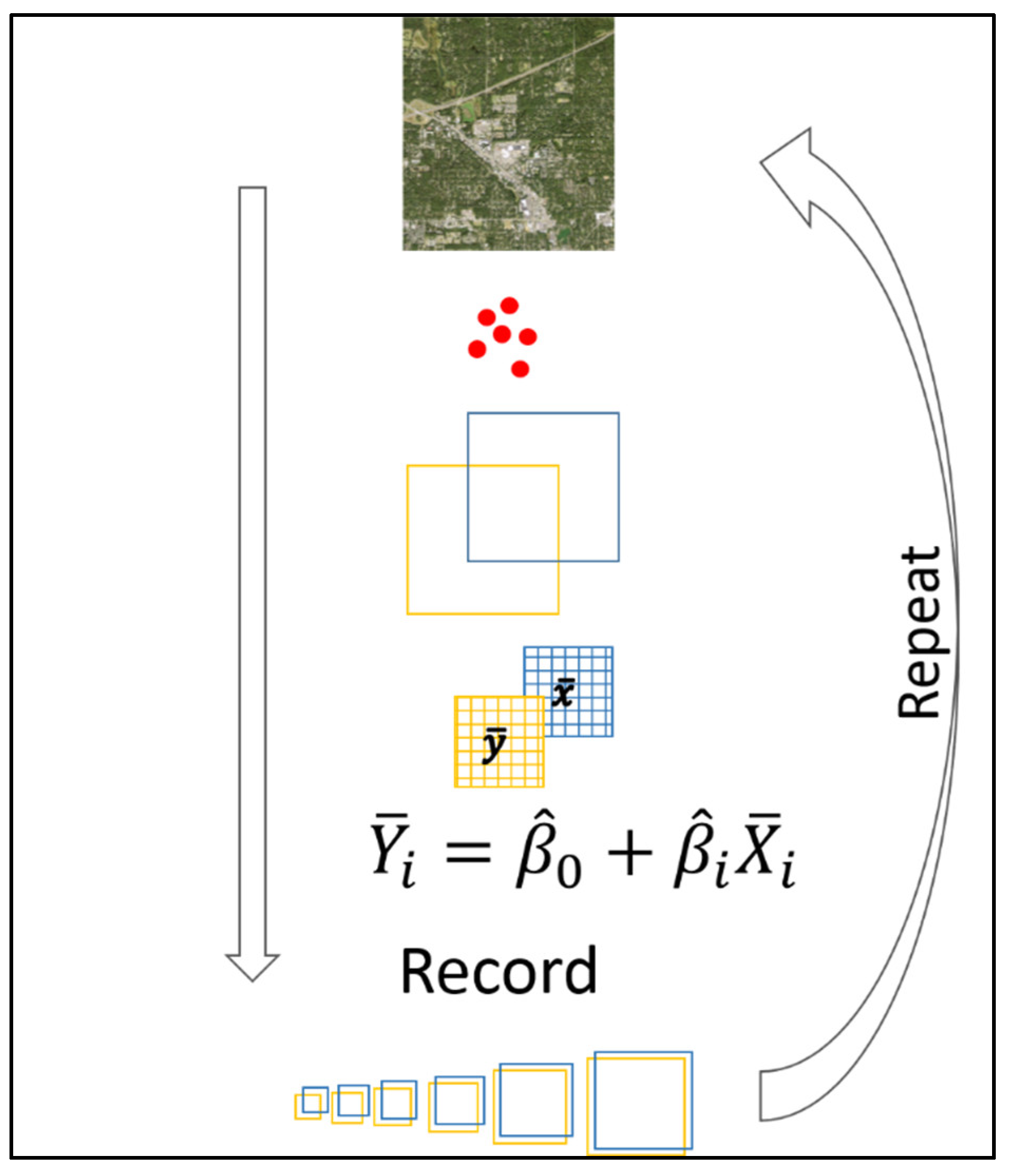
2.2. Overview
2.3. Stage I Simulations
2.4. Stage II Simulations
2.5. Modelling the Impacts of Co-Registration Error
3. Results
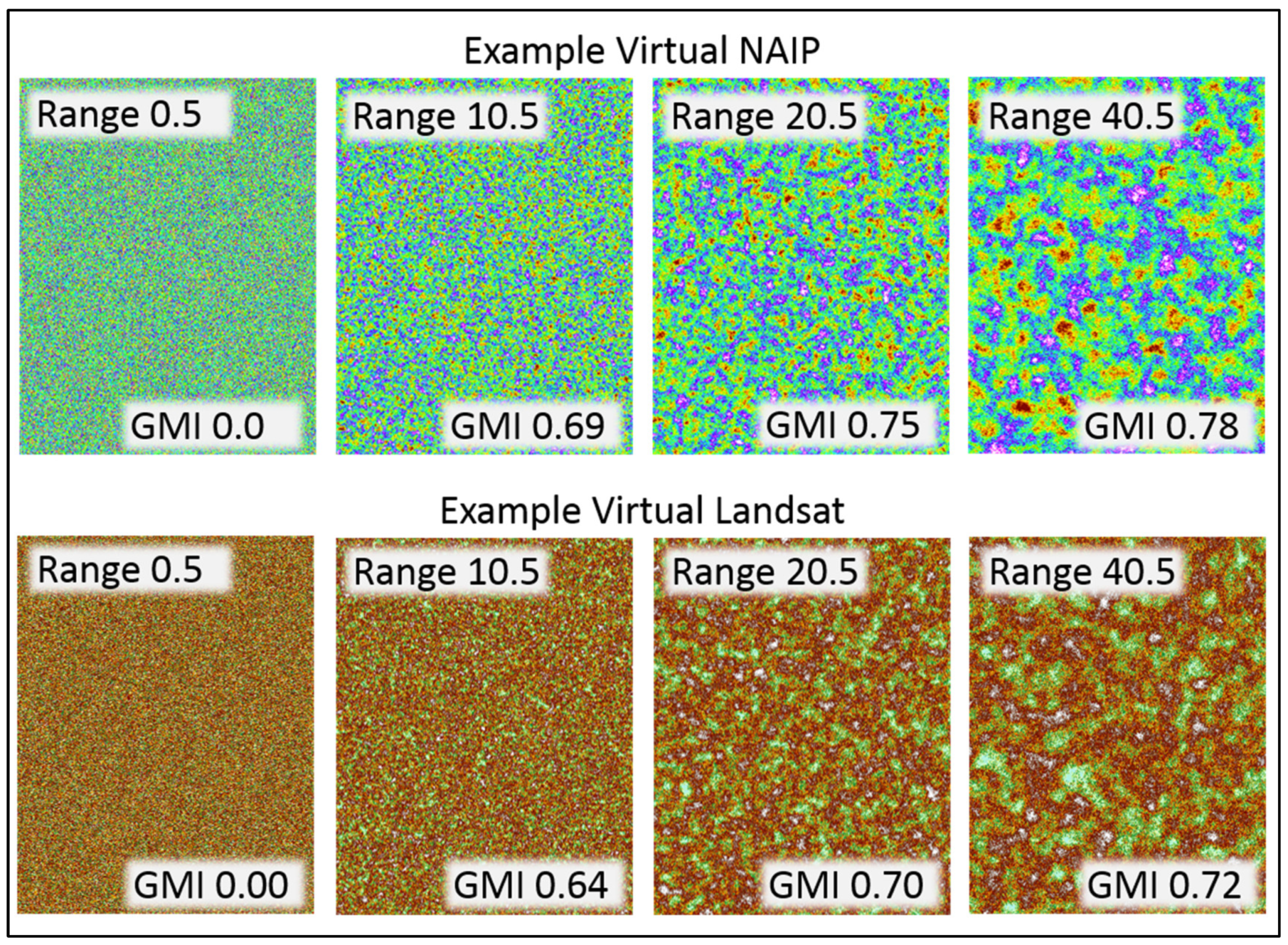
3.1. Datasets
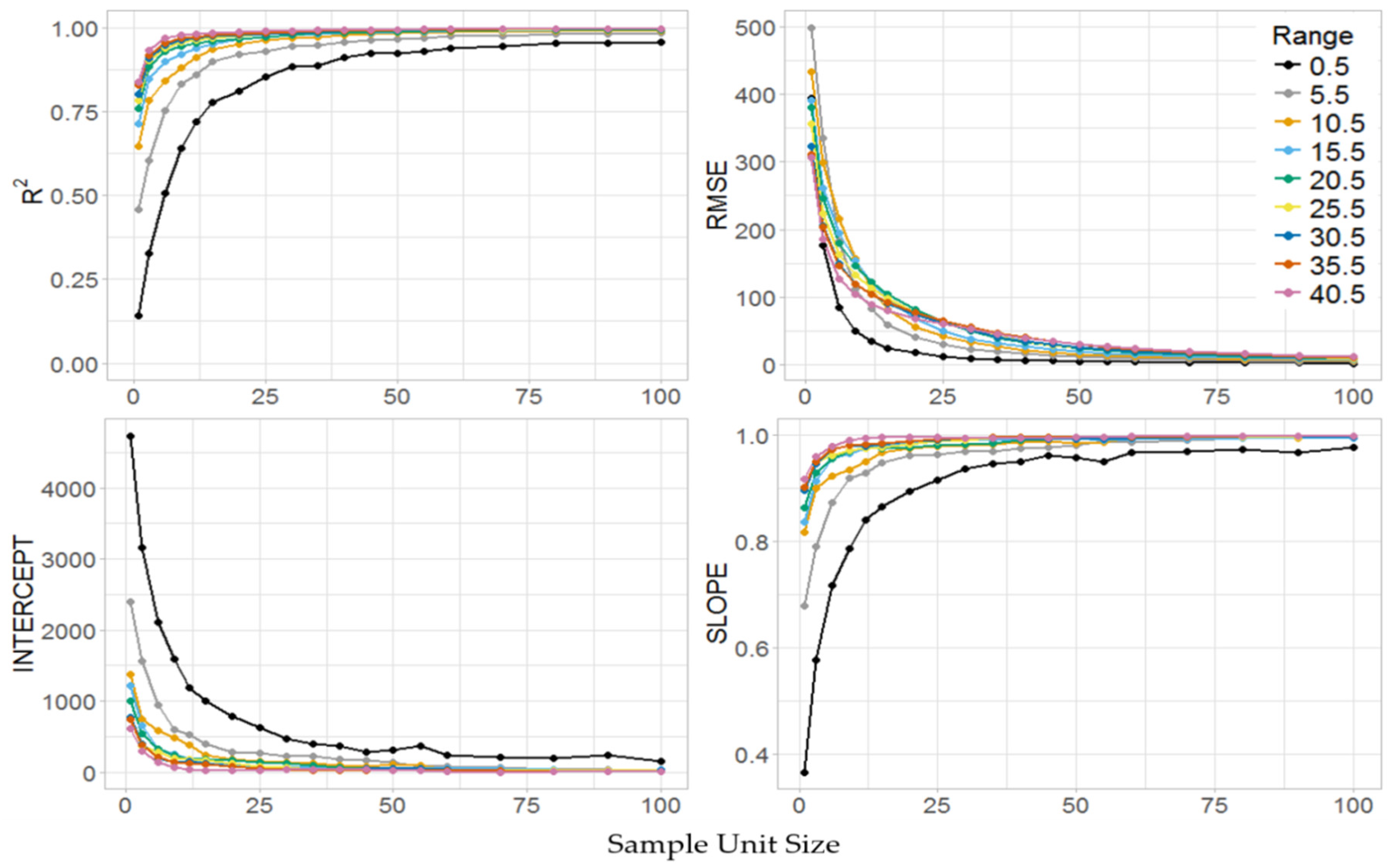
3.2. Stage I
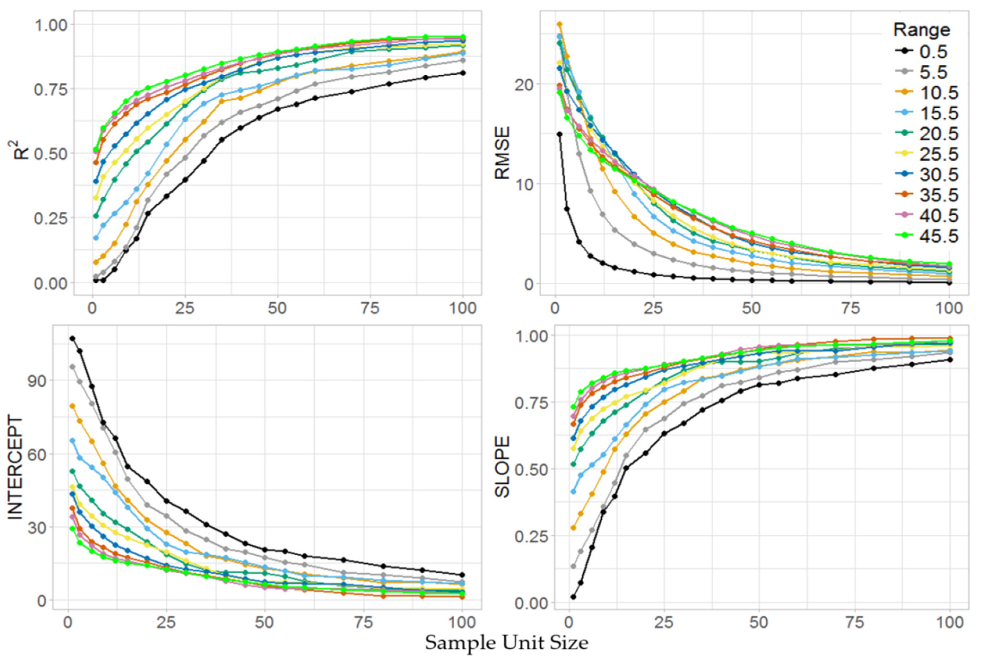
3.3. Stage II
3.4. Model Fitting
4. Discussion
5. Conclusions
Supplementary Materials
Supplementary File 1Author Contributions
Funding
Acknowledgments
Conflicts of Interest
Appendix A
Appendix B

Appendix C


| Application | Data Source | Impact on Model Fit and Estimates |
|---|---|---|
| Mapping forest characteristics using models derived from field data and remotely sensed data. | Landsat imagery | Attenuated estimates and reduction in model fit. The amount depends on the spatial correlation within the imagery, the co-registration error between imagery and field data, and the spatial extent of the field data observations (Table A2). |
| NAIP imagery | Attenuated estimates and reduction in model fit. The amount depends on the spatial correlation within the imagery, the co-registration error between imagery and field data, and the spatial extent of the field data observations (Table A2). | |
| Other remotely sensed data. | Attenuated estimates and reduction in model fit. The amount depends on the spatial correlation within the imagery, the co-registration error between imagery and field data, and the spatial extent of the field data observations. | |
| Change detection derived from multiple images of a given area. | Satellite and aerial based imagery | Attenuated estimates and reduction in model fit. |
| Image radiometric normalization | Satellite and aerial based imagery | Attenuated estimates and reduction in model fit. |
| Image segmentation | Attenuated outputs | Less variation in estimated values potentially reducing the accuracy of the segmentation process. |
| Practitioner use of attenuated spatial data products derived from field plots and remotely sensed imagery. | Attenuated outputs | Mean estimates derived from the entire surface will not be bias. Subsets of the derived surface will be biased and will either over estimate (values < mean) or under estimate (values > mean) the true values. |
| Source | Sample Unit Size (Cells Wide) | GMI | ∆R2 |
|---|---|---|---|
| Landsat 8 | 3 | 0.8 | 0.067 |
| Landsat 8 | 5 | 0.8 | 0.043 |
| Landsat 8 | 9 | 0.8 | 0.026 |
| Landsat 8 | 3 | 0.9 | 0.040 |
| Landsat 8 | 5 | 0.9 | 0.026 |
| Landsat 8 | 9 | 0.9 | 0.016 |
| Landsat 8 | 3 | 0.95 | 0.030 |
| Landsat 8 | 5 | 0.95 | 0.019 |
| Landsat 8 | 9 | 0.95 | 0.012 |
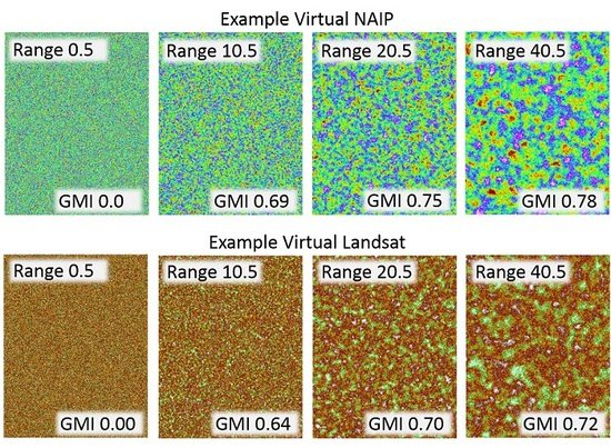
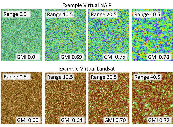
| NAIP | 20 | 0.8 | 0.226 |
| NAIP | 30 | 0.8 | 0.166 |
| NAIP | 40 | 0.8 | 0.131 |
| NAIP | 20 | 0.9 | 0.148 |
| NAIP | 30 | 0.9 | 0.109 |
| NAIP | 40 | 0.9 | 0.088 |
| NAIP | 20 | 0.95 | 0.116 |
| NAIP | 30 | 0.95 | 0.087 |
| NAIP | 40 | 0.95 | 0.070 |
References
- Jensen, J. Remote Sensing of the Environment: An Earth Resource Perspective; Prentice Hall: Upper Saddle River, NJ, USA, 2000; p. 544. [Google Scholar]
- Bechtold, W.A.; Patterson, P.L. (Eds.) The Enhanced Forest Inventory and Analysis Program—National Sampling Design and Estimation Procedures; General Technical Report, SRS-80; Department of Agriculture, Forest Service, Southern Research Station: Asheville, NC, USA, 2005; p. 85. [Google Scholar]
- Omernik, J.; Griffith, G. Ecoregions of the conterminous United States: Evolution of a hierarchical spatial framework. Environ. Manag. 2014, 54, 1249–1266. [Google Scholar] [CrossRef] [PubMed]
- Gesch, D.; Oimoen, M.; Greenlee, S.; Nelson, C.; Steuck, M.; Tyler, D. The National Elevation Dataset. Photogr. Eng. Remote Sens. 2002, 68, 5–11. [Google Scholar]
- Homer, C.; Dewitz, J.; Yang, L.; Jin, S.; Danielson, P.; Xian, G.; Coulston, J.; Herold, N.; Wickham, J.; Megown, K. Completion of the 2011 National Land Cover Database for the conterminous United States-Representing a decade of land cover change information. Photogr. Eng. Remote Sens. 2015, 81, 345–354. [Google Scholar]
- Gandhi, G.; Parthiban, S.; Thummalu, N.; Christy, A. Ndvi: Vegetation Change Detection Using Remtoe Sensing and Gis—A Case Study of Vellori District. Procedia Comput. Sci. 2015, 57, 1199–1210. [Google Scholar] [CrossRef]
- LANDFIRE. Existing Vegetation Type Layer, LANDFIRE 1.1.0, U.S. Department of the Interior, Geological Survey. 2008. Available online: http://landfire.cr.usgs.gov/viewer/ (accessed on 28 April 2018).
- Lowry, J.; Ramsey, R.; Boykin, K.; Bradford, D.; Comer, P.; Falzarano, S.; Kepner, W.; Kirby, J.; Langs, L.; Prior-Magee, J. Southwest Regional Gap Analysis Project: Final Report on Land Cover Mapping Methods; RS/GIS Laboratory, Utah State University: Logan, UT, USA, 2005. [Google Scholar]
- Escuin, S.; Navarro, R.; Fernandez, P. Fire severity assessment buy using NBR (Normalized Burn Ratio) and NDVI (Normalized Difference Vegetation Index) derived from LANDSAT TM/ETM images. Int. J. Remote Sens. 2008, 29, 1053–1073. [Google Scholar] [CrossRef]
- Davids, C.; Doulgeris, A. Unsupervised change detection of multitemporal Landsat imagery to identify changes in land cover following the Chernobyl accident. In Proceedings of the Geoscience and Remote Sensing Symposium, Barcelona, Spain, 8–11 July 2008; pp. 3486–3489. [Google Scholar]
- Weng, Q.; Fu, P.; Gao, F. Generating daily land surface temperature at Landsat resolution by fusing Landsat and MODIS data. Remote Sens. Environ. 2014, 145, 55–67. [Google Scholar] [CrossRef]
- Turner, M.; Gardner, G.; O’Neil, R. Landscape Ecology in Theory and Practice: Pattern and Process; Springer: New York, NY, USA, 2001; p. 406. [Google Scholar]
- Pietsch, M. Contribution of connectivity metrics to the assessment of biodiversity—Some methodological considerations to improve landscape planning. Ecol. Indic. 2018, 94, 116–127. [Google Scholar] [CrossRef]
- Stancioiu, P.; Nita, M.; Lazar, G. Forestland connectivity in Romania—Implications for policy and management. Land Use Policy 2018, 76, 487–499. [Google Scholar] [CrossRef]
- Lechner, M.; Harris, R.; Doerr, V.; Doerr, E.; Drielsma, M.; Lefroy, E. From static connectivity modelling to scenario-based planning at local and regional scales. J. Nat. Conserv. 2015, 28, 78–88. [Google Scholar] [CrossRef]
- Shafer, G. Land use planning: A potential force for retaining habitat connectivity in the Greater Yellowstone Ecosystem an dBeyon. Glob. Ecol. Conserv. 2015, 3, 256–278. [Google Scholar] [CrossRef]
- Ersoy, E.; Jorgensen, A.; Warren, P. Identifying multispecies connectivity corridors and the spatial pattern of the landscape. Urban For. Urban Green. 2018. [Google Scholar] [CrossRef]
- Hogland, J.; Anderson, N. Function Modeling Improves the Efficiency of Spatial Modeling Using Big Data from Remote Sensing. Big Data Cogn. Comput. 2017, 1, 3. [Google Scholar] [CrossRef]
- Hogland, J.; Anderson, N.; St. Peters, J.; Drake, J.; Medley, P. Mapping Forest Characteristics at Fine Resolution across Large Landscapes of the Southeastern United States Using NAIP Imagery and FIA Field Plot Data. Int. J. Geo-Inf. 2018, 7, 140. [Google Scholar] [CrossRef]
- Masek, J.; Hayes, D.; Hughes, M.; Healey, S.; Turner, D. The role of remote sensing in process-scaling studies of managed forest ecosystems. For. Ecol. Manag. 2015, 355, 109–123. [Google Scholar] [CrossRef]
- Hogland, J.; Anderson, N.; Chung, W. New Geospatial Approaches for Efficiently Mapping Forest Biomass Logistics at High Resolution over Large Areas. Int. J. Geo-Inf. 2018, 7, 156. [Google Scholar] [CrossRef]
- St. Peters, J.; Hogland, J.; Anderson, N.; Drake, J.; Medley, P. Fine resolution probabilistic land cover classification of landscapes in the southeastern United States. Int. J. Geo-Inf. 2018, 7, 107. [Google Scholar] [CrossRef]
- Graves, S.; Caughlin, T.; Asner, G.; Bohlman, S. A tree-based approach to biomass estimation from remote sensing data in a tropical agricultural landscape. Remote Sens. Environ. 2018, 218, 32–43. [Google Scholar] [CrossRef]
- Faga, M.; Morton, D.; Cook, B.; Masek, J.; Zhao, F.; Nelson, R.; Huang, C. Mapping pine plantation sin the southeastern U.S. using structural, spectral, and temporal remote sensing data. Remote Sens. Environ. 2018, 216, 415–426. [Google Scholar] [CrossRef]
- Cheshner, A. The effect of measurement error. Biometrika 1991, 78, 451–462. [Google Scholar] [CrossRef]
- Fuller, W. Measurement Error Models; Wiley: New York, NY, USA, 1987; p. 500. [Google Scholar]
- Greenberg, J.; Dobrowski, S.; Ustin, S. Shadow allometry: Estimating tree structural parameters using hyperspatial image analysis. Remote Sens. Environ. 2005, 97, 15–25. [Google Scholar] [CrossRef]
- Sheridan, R.; Popescu, S.; Gatziolis, D.; Morgan, C.; Ku, W. Modeling Forest Above ground Biomass and Volume Using Airborne LiDAR metrics and Forest Inventory and Analysis Data in the Pacific Northwest. Remote Sens. 2015, 7, 229–255. [Google Scholar] [CrossRef]
- Frazer, G.; Magnussen, S.; Wulder, M.; Niemann, K. Simulated impact of sample plot size and co-registration error on the accuracy of and uncertainty of LiDAR-derived estimates of forest stand biomass. Remote Sens. Envrion. 2011, 115, 636–649. [Google Scholar] [CrossRef]
- Bobakken, T.; Naesset, E. Assessing effects of positioning errors and sample plot size on biophysical stand properties derived from airborne laser scanner data. Can. J. For. Res. 2009, 39, 1036–1052. [Google Scholar] [CrossRef]
- Saarela, S.; Schnell, S.; Tuominen, S.; Balazs, A.; Hyyppa, J.; Grafstrom, A.; Stahl, G. Effects of positional errors in model–assisted and model-based estimation of growing stock volume. Remote Sens. Environ. 2016, 172, 101–108. [Google Scholar] [CrossRef]
- Van Niel, T.; McVicar, T.; Li, L.; Gallant, J.; Yang, Q. The impact of misregistration on SRTM and DEM image differences. Remote Sens. Environ. 2008, 112, 2430–2442. [Google Scholar] [CrossRef]
- Moran, P. Notes on Continuous Stochastic Phenomena. Biometrika 1950, 37, 17–23. [Google Scholar] [CrossRef] [PubMed]
- Core Team. R: A Language and Environment for Statistical Computing; R Foundation for Statistical Computing: Vienna, Austria, 2014; Available online: http://www.R-project.org/ (accessed on 28 April 2018).
- Hijmans, R.; Etten, J. Raster: Geographic Analysis and Modeling with Raster Data. R Package Version 2.0-12. 2012. Available online: http://CRAN.R-project.org/package=raster (accessed on 24 September 2018).
- Pebesma, E. Multivariable geostatistics in S: The gstat package. Comput. Geosci. 2004, 30, 683–691. [Google Scholar] [CrossRef]
- Gräler, B.; Pebesma, E.; Heuvelink, G. Spatio-Temporal Interpolation using gstat. R J. 2016, 8, 204–218. [Google Scholar]
- Landsat. Landsat Project Description. 2018. Available online: https://landsat.usgs.gov/landsat-project-description (accessed on 27 April 2018).
- National Agriculture Imagery Program [NAIP]. National Agriculture Imagery Program (NAIP) Information Sheet. Available online: http://www.fsa.usda.gov/Internet/FSA_File/ naip_info_sheet_2013.pdf (accessed on 14 May 2014).
- Cressie, N. Statistics for Spatial Data Revised Edition; Wiley Classics Library, John Wiley: Hoboken, NJ, USA, 2015; p. 928. [Google Scholar]
- Loveland, T.; Irons, J. Landsat 8: The plans, the reality, and the legacy. Remote Sens. Environ. 2016, 185, 1–6. [Google Scholar] [CrossRef]
- Beyerhelm, C. Head-to-Head Comparison of Four SiRF-Based GPS Receivers. 2009 Report. Available online: https://www.fs.fed.us/database/gps/documents/SiRFComp.pdf (accessed on 24 September 2018).
- Forest Inventory and Analysis Program [FIA]. Forest Inventory and Analysis National Core Field Guide: Field Data Collection Procedures for Phase 2 Plots. Version 6.0. Vol. 1; Internal Report; U.S. Department of Agriculture Forest: Washington, DC, USA, 2012. Available online: http://www.fia.fs.fed.us/library/field-guides-methods-proc/docs/2013/Core%20FIA%20P2%20field%20guide_6-0_6_27_2013.pdf (accessed on 5 June 2014).
- Cribari-Neto, F.; Zeileis, A. Beta Regression in R. J. Stat. Softw. 2010, 34. [Google Scholar] [CrossRef]
- Akaike, H. Information theory and an extension of the maximum likelihood principle. In Selected Papers of Hirotugu Akaike; Petrov, B.N., Csake, F., Eds.; Springer: New York, NY, USA, 1973; pp. 267–281. [Google Scholar]
- Akaike, H. A new look at the statistical model identification. IEEE Trans. Autom. Control 1974, 19, 716–723. [Google Scholar] [CrossRef]
- Patterson, P.L.; Williams, M.S. Effects of registration error between remotely sensed and ground data on estimators of forest area. For. Sci. 2003, 49, 110−118. [Google Scholar]
- Zhang, M.; Lin, H.; Zeng, S.; Li, J.; Shi, J.; Wang, G. Impacts of plot location errors on accuracy of mapping and scaling up aboveground forest carbon using sample plot and landsat tm data. IEEE Geosci. Remote Sens. Lett. 2013, 10, 1483–1487. [Google Scholar] [CrossRef]
- Frost, C.; Thompson, S. Correcting for regression dilution bias: Comparison of methods for a single predictor. J. R. Statist. Soc. A 2000, 163, 173–189. [Google Scholar] [CrossRef]


| Name | Label | MDN | Sill | Range | Nugget | GMI |
|---|---|---|---|---|---|---|
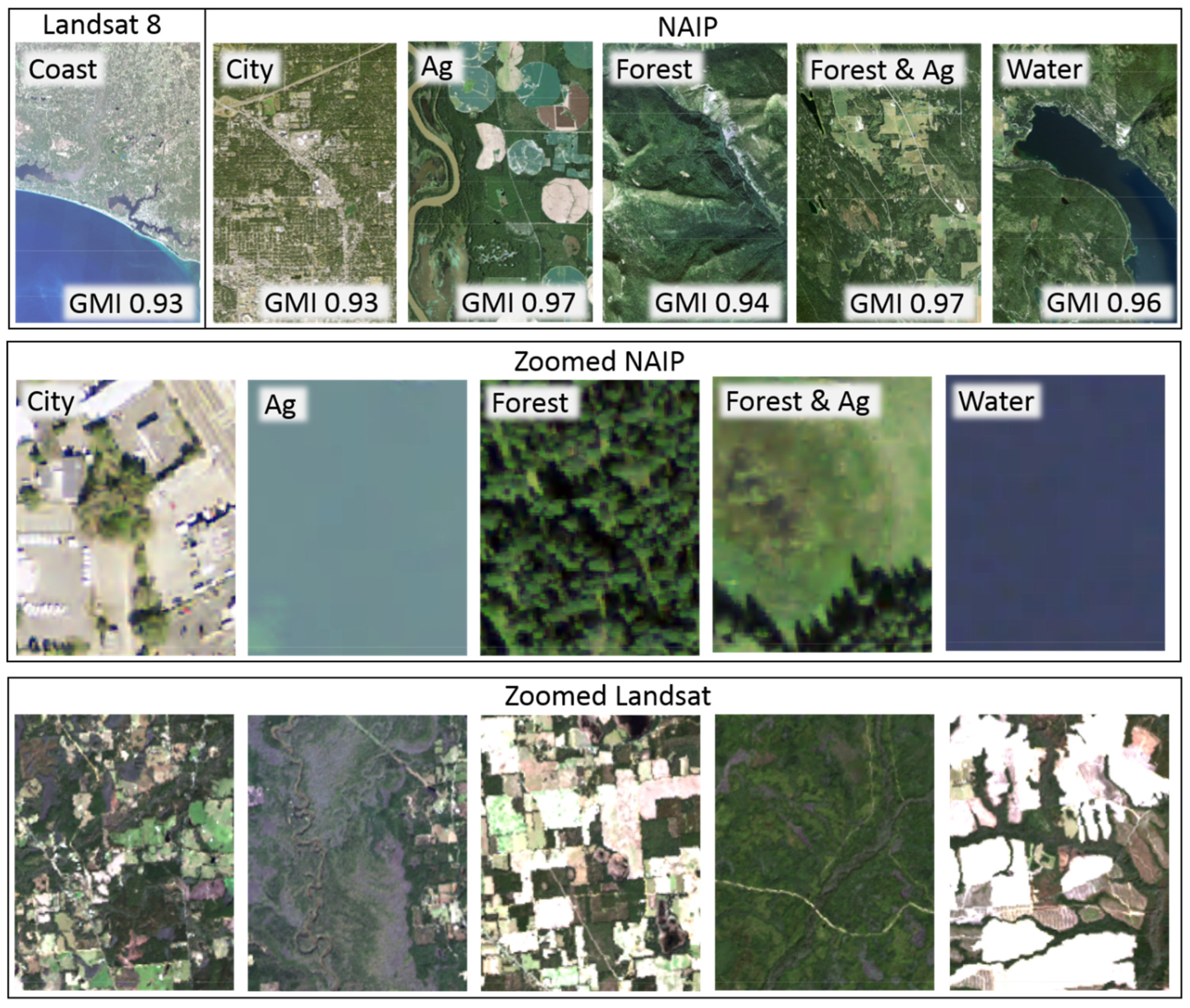
| Landsat 8 Coast | Coast | 7478.1 | 552,790.7 | 40.5 | 180,321.3 | 0.93 |
| NAIP City | City | 140.2 | 1630.3 | 30.1 | 348.7 | 0.93 |
| NAIP Agriculture | Ag | 115.7 | 449.3 | 46.0 | 161.0 | 0.97 |
| NAIP Forest | Forest | 86.3 | 525.0 | 31.2 | 187.4 | 0.94 |
| NAIP Forest & Agriculture | Forest & Ag | 119.0 | 593.9 | 41.9 | 78.7 | 0.97 |
| NAIP Forest & Water | Water | 88.9 | 548.3 | 33.8 | 113.9 | 0.96 |
| Model | Equation | Slope | R2 | RSE | F-Stat | P-Value |
|---|---|---|---|---|---|---|
| Landsat 8 | 1.008 | 0.9984 | 0.03456 | 11440 | <0.001 | |
| NAIP | 1.035 * | 0.9983 | 0.02364 | 10330 | <0.001 |
| Model | Rank | Source | Predictors | AIC | ΔAIC |
|---|---|---|---|---|---|
| 1 | 6 | Landsat 8 | −1723.823 | −651.018 | |
| 2 | 4 | Landsat 8 | −1920.781 | −454.06 | |
| 3 | 3 | Landsat 8 | −1938.580 | −436.261 | |
| 4 | 5 | Landsat 8 | −1870.267 | −504.574 | |
| 5 | 2 | Landsat 8 | −2368.824 | −6.017 | |
| 6 | 1 | Landsat 8 | −2374.841 | 0 | |
| 1 | 6 | NAIP | −1086.606 | −681.595 | |
| 2 | 5 | NAIP | −1469.469 | −298.732 | |
| 3 | 3 | NAIP | −1494.508 | −273.693 | |
| 4 | 4 | NAIP | −1193.989 | −574.212 | |
| 5 | 2 | NAIP | −1728.674 | −39.527 | |
| 6 | 1 | NAIP | −1768.201 | 0 |
| Model | N | Intercept + | LSS + | EGIM + | EGMI * LSS + | Pseudo R2 [45] | P-Value |
|---|---|---|---|---|---|---|---|
| Landsat 8 | 304 | −3.743 | 1.089 | 2.423 | −0.085 | 0.918 | <0.001 |
| NAIP | 570 | −9.364 | 1.883 | 3.481 | −0.419 | 0.8255 | <0.001 |
© 2019 by the authors. Licensee MDPI, Basel, Switzerland. This article is an open access article distributed under the terms and conditions of the Creative Commons Attribution (CC BY) license (http://creativecommons.org/licenses/by/4.0/).
Share and Cite
Hogland, J.; Affleck, D.L.R. Mitigating the Impact of Field and Image Registration Errors through Spatial Aggregation. Remote Sens. 2019, 11, 222. https://doi.org/10.3390/rs11030222
Hogland J, Affleck DLR. Mitigating the Impact of Field and Image Registration Errors through Spatial Aggregation. Remote Sensing. 2019; 11(3):222. https://doi.org/10.3390/rs11030222
Chicago/Turabian StyleHogland, John, and David L.R. Affleck. 2019. "Mitigating the Impact of Field and Image Registration Errors through Spatial Aggregation" Remote Sensing 11, no. 3: 222. https://doi.org/10.3390/rs11030222
APA StyleHogland, J., & Affleck, D. L. R. (2019). Mitigating the Impact of Field and Image Registration Errors through Spatial Aggregation. Remote Sensing, 11(3), 222. https://doi.org/10.3390/rs11030222