Article

Methane Mapping with Future Satellite Imaging Spectrometers

1
Department of Geography, University of California Santa Barbara, Santa Barbara, CA 93106, USA
2
Department of Geography, University of Utah, Salt Lake City, UT 84112, USA
3
Jet Propulsion Laboratory, California Institute of Technology, Pasadena, CA 91109, USA
4
Scientific Computing and Imaging Institute, University of Utah, Salt Lake City, UT 84112, USA
5
Office for Research, Innovation and Impact, University of Arizona, Tucson, AZ 85721, USA
*
Author to whom correspondence should be addressed.
Remote Sens. 2019, 11(24), 3054; https://doi.org/10.3390/rs11243054
Submission received: 14 November 2019 / Revised: 6 December 2019 / Accepted: 13 December 2019 / Published: 17 December 2019
(This article belongs to the Special Issue State-of-the-Art Remote Sensing in North America 2019)

Abstract

:
This study evaluates a new generation of satellite imaging spectrometers to measure point source methane emissions from anthropogenic sources. We used the Airborne Visible and Infrared Imaging Spectrometer Next Generation(AVIRIS-NG) images with known methane plumes to create two simulated satellite products. One simulation had a 30 m spatial resolution with ~200 Signal-to-Noise Ratio (SNR) in the Shortwave Infrared (SWIR) and the other had a 60 m spatial resolution with ~400 SNR in the SWIR; both products had a 7.5 nm spectral spacing. We applied a linear matched filter with a sparsity prior and an albedo correction to detect and quantify the methane emission in the original AVIRIS-NG images and in both satellite simulations. We also calculated an emission flux for all images. We found that all methane plumes were detectable in all satellite simulations. The flux calculations for the simulated satellite images correlated well with the calculated flux for the original AVIRIS-NG images. We also found that coarsening spatial resolution had the largest impact on the sensitivity of the results. These results suggest that methane detection and quantification of point sources will be possible with the next generation of satellite imaging spectrometers.

Graphical Abstract

1. Introduction

Methane is a prominent greenhouse gas and is responsible for about 20% of all atmospheric radiative forcing [1,2]. As our planet continues to warm due to radiative forcing caused by greenhouse gases, understanding, monitoring, and reducing these emissions will become increasingly important. However, there remains a high level of uncertainty regarding the magnitude of methane sources and sinks globally [2,3]. Anthropogenic sources, which make up 50–65% of all methane emissions, mostly come from the energy, waste, and agriculture sectors [2,4]. These are generally point sources, or emissions emanating from a single easily identifiable source like a gas storage tank or a landfill [5,6]. Although these sectors can also contain diffuse sources, or emissions coming from a larger area, a few point sources can dominate the emissions budget. Identifying emission sources and quantifying their rates can improve regional greenhouse gas budgets and mitigation strategies [6,7].
This study investigates the potential to use a future generation of Earth observing satellites to map methane emissions. Past and present satellite missions measure atmospheric methane, but lack the fine spatial resolution needed to measure individual point sources. These sensors, such as the Atmospheric Infrared Sounder (AIRS), SCanning Imaging Absorption SpectroMeter for Atmospheric CHartographY (SCIAMACHY), TROPOspheric Monitoring Instrument (TROPOMI), and the Greenhouse gas Observing Satellite (GOSAT), can accurately characterize the global and regional distributions of methane, but only at spatial resolutions between 7 and 60 km [8,9,10,11,12]. More recently, GHGsat demonstrated the ability to map methane plumes at a resolution as fine as 50 m [13,14]. Future satellites may be able to detect methane at even finer spatial resolutions.
In the coming decade, there is strong interest in a new generation of Earth observing satellites equipped with Visible and Shortwave Infrared (VSWIR) imaging spectrometers [15]. VSWIR imaging spectrometers typically measure between 380 and about 2500 nm with between 5 to 10 nm spectral spacing [6,16,17,18,19]. These imaging spectrometers are sensitive to gas absorption features, which allows for the detection and quantitative mapping of methane, carbon dioxide, and water vapor [16,20,21,22]. In 2019, the Italian space agency launched the Hyperspectral Precursor and Application Mission (PRISMA), a medium resolution imaging spectrometer [23,24]. In 2020, the German space agency plans to launch the Environmental Mapping and Analysis Program (EnMAP) [25] and the Japanese government plans to launch the Hyperspectral Imager Suite (HISUI) [26], both of which are spaceborne imaging spectrometers.The National Aeronautics and Space Administration (NASA) plans to launch the Earth Surface Mineral Dust Source Investigation (EMIT) to the International Space Station (ISS) in 2021. NASA’s Surface Biology and Geology investigation is likely to include an imaging spectrometer that could launch as early as 2025 [27]. None of these sensors are being designed for gas mapping, but if these instruments can be used for methane mapping, the global monitoring of greenhouse gases will drastically improve.
Recent work with a current satellite VSWIR imaging spectrometer and airborne imaging spectrometer data have provided a testbed for evaluating point source methane detection and measurements with these types of instruments [16,18,20,22,28]. The Hyperion imaging spectrometer on board the EO-1 satellite successfully detected the accidental methane release at Aliso Canyon [28], despite the age of the sensor and low signal-to-noise ratio (SNR). The Airborne Visible and Infrared Imaging Spectrometer Next Generation instrument (AVIRIS-NG), detected, geolocated, and quantified over 500 methane point sources throughout California from the oil and gas, manure management, and waste management sectors [7]. Across each sector, a small number of point sources contributed the majority of observed methane emissions, demonstrating the importance of observing point sources.
While none of the proposed future imaging spectrometers are explicitly designed to map greenhouse gases, given their design and the prior successful work using similar airborne sensors to map methane, the upcoming generation of spaceborne imaging spectrometers has great potential for global mapping of near-surface methane emissions. This study examines the possibility of using these future sensors to monitor emissions from three of the largest anthropogenic methane sectors: oil/gas, waste management, and agriculture.

2. Methods

In order to test the capability of future sensors for methane mapping, we resampled AVIRIS-NG data to create a simulated satellite product (Figure 1) and then tested methane retrievals using this new product. We based our simulated satellite data on the sensor design for the upcoming EMIT mission [29]. The EMIT sensor design favors radiometric sensitivity over spatial resolution, leading to a 60 m spatial sampling that is slightly coarser than the 30 m spatial sampling slated for many orbital VSWIR sensors. Therefore, we simulated two sensor designs. The first was characteristic of a hypothetical future NASA mission after EMIT as well as those already operating or planned for launch by other space agencies. It has a 30 m spatial resolution with lower SNR. The second was a direct analogue of the EMIT instrument, with a 60 m spatial resolution and a higher SNR. Both simulations are important for understanding the methane mapping potential for NASA’s future generation of sensors. The following section describes the original AVIRIS-NG data used, the process to resample it to a simulated satellite product, and the methane retrieval algorithm.

2.1. Imagery

AVIRIS-NG is an airborne imaging spectrometer that measures radiance in the visible through shortwave-infrared (SWIR). It measures in the spectral range from about 380 to 2500 nm with a 5 nm spectral sampling [30,31,32]. AVIRIS-NG has a 34° field of view and a one milliradian instantaneous field-of-view that results in spatial resolutions ranging between approximately 1 and 8 meters, depending on the height of the aircraft. The AVIRIS-NG data used in this study were collected in 2016 and 2017 throughout California as part of the California Methane Survey and an image from a 2018 controlled release experiment [33]. We selected images of plumes from a landfill, a dairy, a dairy digester, a wastewater treatment facility, and oil/gas infrastructure. In this study, eight examples of plumes (Table 1), one or more from each source, were resampled to satellite specifications using the methods described below.

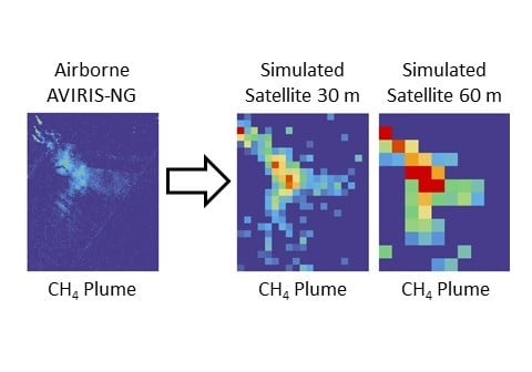
2.2. Simulated Satellite Images

2.2.1. Aircraft to Top-of-Atmosphere

To simulate the additional atmosphere between the original aircraft height and the top of the atmosphere (TOA), we used MODerate resolution atmospheric TRANsmission 6 (MODTRAN6) to simulate one-way transmittance between the two heights [34]. Each transmittance simulation was generated with the aircraft height, latitude, longitude, day, and time of day of the original AVIRIS-NG flight. In addition, we assumed a background carbon dioxide, methane, and water vapor profile. Pixel radiance values from each image were multiplied by each simulated transmittance spectrum. For more details on the MODTRAN6 inputs and an example of a radiance spectrum adjusted to TOA, please see Appendix A.

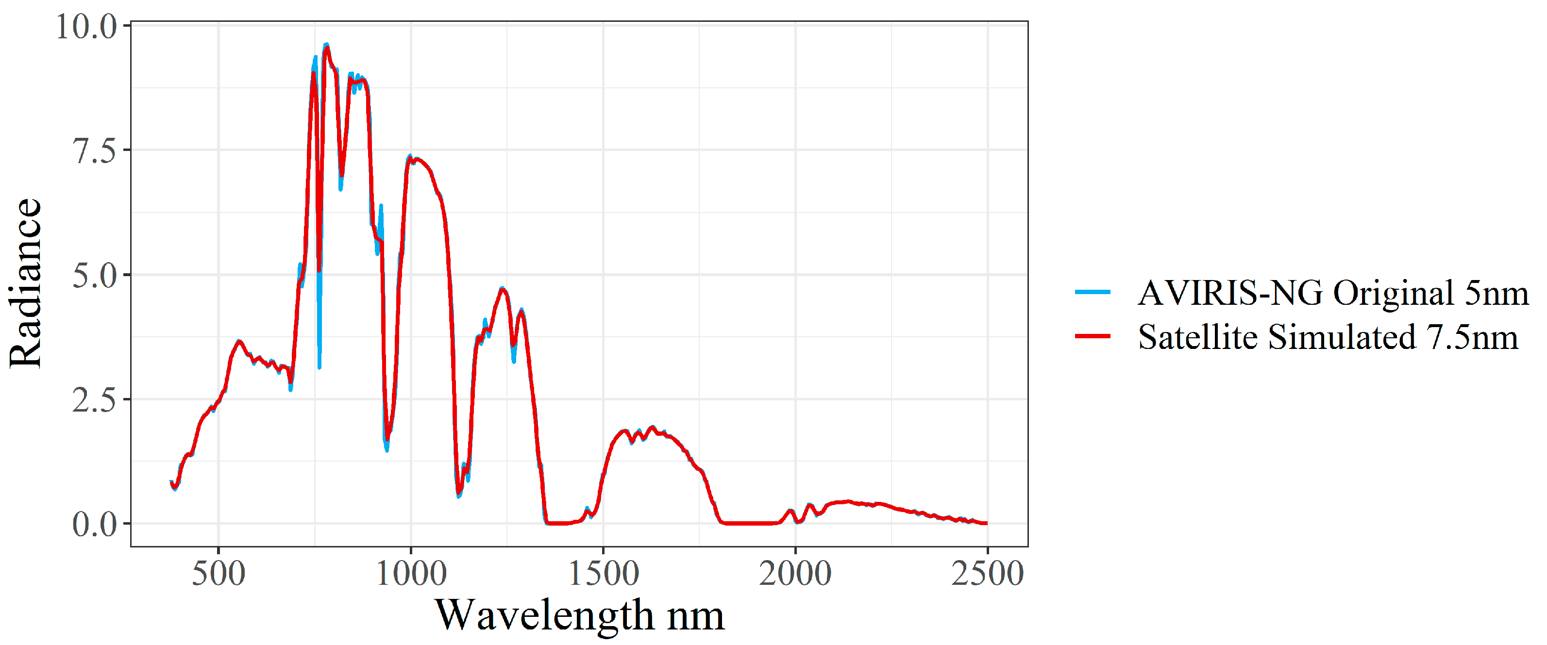
2.2.2. Spectral Resampling

The exact band centers and full width half maximum (FWHM) for EMIT are still to be determined. However, EMIT will most likely have a 7.4 nm spectral sampling with an 8.2 to 8.8 nm FWHM. We resampled spectra from AVIRIS-NG radiance images using a Gaussian convolution with band centers and FWHM based on these specifications. In total, the resampled spectra had 288 bands between 376.4 and 2500 nm.

2.2.3. Resample Spatial Resolution

Each image was resampled to 30 m and 60 m spatial resolutions using Gaussian resampling. The stated spatial resolution represents the full-width half maximum of the Gaussian function, with the x-y coordinates for each AVIRIS-NG pixel center used to calculate each pixel’s weighting for resampling. The original unorthorectified AVIRIS-NG images were used for resampling, but pixel coordinate information allowed the creation of orthorectified 30 m and 60 m output images.

2.2.4. Sensor Noise

The SNR from AVIRIS-NG is higher than the proposed SNR for the EMIT sensor and in addition, after spatial and spectrally resampling the data, some of the noise from the original AVIRIS-NG data is reduced through averaging. Therefore, adding sensor noise back into the data is critical for accurately modeling satellite data. To properly model the SNR of the satellite sensors, a noise component aimed at mimicking expected sensor noise was added to the radiance. Modeled sensor noise comes from two main components: photon noise (PN) and constant noise (CN). PN increases as the number of photons hitting a detector increases, and scales with the square root of radiance. CN is mainly associated with electronics and quantization in the signal chain. A primary contributor is “read noise”, caused by the analog-to-digital conversion as the instrument digitally records the signal, and this parameter can be modeled as constant across wavelengths and pixels. To calculate PN, we first converted the spectral radiance to the total number of photons and then multiplied it by the etendue (G), which is calculated based on the area of the emitting source (in this case, the Sun) times the solid angle, band FWHM, integration time (τ), and the system transmittance factor (T):
P N = L λ   ×   ( λ h c )   ×   G   ×   FWHM   ×   τ   ×   T
where PN is the photon noise; Lλ is the radiance at each wavelength in each pixel; λ is the wavelength; and hc is Planck’s constant times the speed of light. The AVIRIS-NG CN is 100 photons, therefore the same value was used for this simulation. The total noise was calculated as follows:
T N = ( P N 2 + C N 2 )
where TN is the total noise. The total noise was then converted back to radiance units by substituting TN for PN in Equation (1) and inverting. TN converted to radiance was then multiplied by a random number from a Gaussian distribution with a mean of 0 and standard deviation of 1, then added to the original radiance for each wavelength for each pixel. PN increases with increasing radiance; for low radiance values, CN dominates the total noise and for higher radiance values, PN dominates. For the 60 m image, we multiplied PN by the square root of 2. The SNR was calculated by dividing the signal by the noise. In this case, the signal was the number of photons and the noise is the total noise. The resulting average SNR for the 30 m simulated satellite images in the SWIR (2100 nm–2500 nm) was 214 and the average SNR for the 60 m simulated satellite images in the SWIR was 484. Figure 2 shows the full spectrum SNR for the two simulations.

2.3. Matched Filter Methane Retrieval

The methane enhancement above the background for each pixel was estimated using an iterative matched filter technique tuned with a methane unit absorption spectrum [19,35,36,37]. This iterative method included additional optimization factors that correct for spatially varying surface albedo. In addition, a 1 sparsity prior was included to reflect the expectation that methane enhancement is a rare occurrence within an image. This sparse approach is similar to methods employed in compressed sensing techniques for the reduction of acquisition time or improved resolution in fields as varied as medical imaging, radio astronomy, and electron microscopy [38,39,40,41,42]. The iterative technique required for solving this sparse optimization problem additionally produces the explicit removal of any methane absorption signal from the background covariance matrix; failure to remove this signal is detrimental to matched filter techniques [36,37,43,44].
This iterative matched filter with sparsity and albedo correction was applied to the AVIRIS-NG images and simulated 30 m and 60 m images. For all scenes, the sparse matched filter was run for 30 iterations, which includes an additional 50% margin over the 20 iterations that produced initial observable convergence of the optimization energy. The number of iterations was based on observations of convergence from a test dataset. The methane unit absorption spectrum for each scene was computed from the change in radiance corresponding to a change in methane concentration in MODTRAN6 with each scene’s sensor height and solar zenith angle. The albedo correction factor was estimated by the ratio of a pixel’s radiance to the mean radiance in the scene. For the original AVIRIS-NG data, the matched filter was applied to groups of five adjacent columns, corresponding to adjacent detectors of the AVIRIS-NG instrument. This grouping improved the covariance estimate used by the matched filter to describe the background by suppressing artifacts from non-uniformity among detector elements [19]. For the simulated satellite images, column artifacts were averaged out by spatial resampling, and therefore the matched filter was applied to the entire image.
The resulting methane enhancement image is measured in ppm-m, where ppm represents concentration and m represents the path length over which absorption occurs. Due to this algorithm’s sparsity prior, many pixels are reported to have no methane enhancement above the background. This allows for interpreting the enhancement values as a detection result (presence/absence of methane for a positive/zero enhancement value). We also consider the resulting images as a quantitative retrieval directly from the per-pixel methane concentration. For more information on the retrieval algorithm please see Foote et. al., In Review [45].

2.4. Integrated Mass Enhancement

The integrated mass enhancement (IME) is the sum of all the methane enhancement above the background concentration present in each plume. To calculate the IME, we first need to identify the pixels associated with the plume and filter out spurious signals. We applied a 200 ppm-m threshold to filter out any potential spurious signals. The 200 ppm-m threshold was determined by reviewing the mean and standard deviation for the matched filter outputs. A 200 ppm-m value represents a round average of one standard deviation below the average mean of the enhanced pixels. To further filter out spurious signals, we calculated the number of pixels in contiguous clusters, any clusters below a certain threshold were filtered out. For the original AVIRIS-NG images, any clusters below 350 contiguous pixels were filtered out. For the 30 m satellite simulation, clusters below four pixels were filtered out and for the 60 m satellite simulation, clusters below two pixels were filtered out. Different thresholds were used for some cases based on empirical adjustments and are documented in Appendix A. We then calculated an integrated mass enhancement (IME) or the sum of the methane present in each plume [6] as follows:
IME   =   k i = 0 n α ( i ) S ( i )
where α is the methane value in ppm-m for the n pixels in the plume over the pixel area S and the constant k is used to convert to methane mass units [6].

2.5. Flux Estimate

A simple flux estimate can be calculated using the IME, the length of the plume, and the wind speed. The methods for calculating the IME are listed above. To calculate the length of the plume, we identified the two pixels in the plume with the furthest distance and calculated the Euclidean distance between the two pixels. HRRRv3 10 m wind fields in forecast mode were used to estimate wind speeds for the location and time of each AVIRIS-NG scene [46,47]. Using the 3 km grid product, an average wind speed and standard deviation was calculated using a total of 27 HRRRv3 grid cells, a 3 × 3 box centered on the source for three time-steps (plume detection time ±1 hour). The equation for the flux is as follows:
F l u x   =   IME l s
where IME is the amount of methane in kg (calculated above); l is the plume length in meters; s is the wind speed meter/hour; and the resulting flux in the units of kg/hour. The uncertainties for the flux estimates result from uncertainties in the wind speeds.

3. Results and Discussion

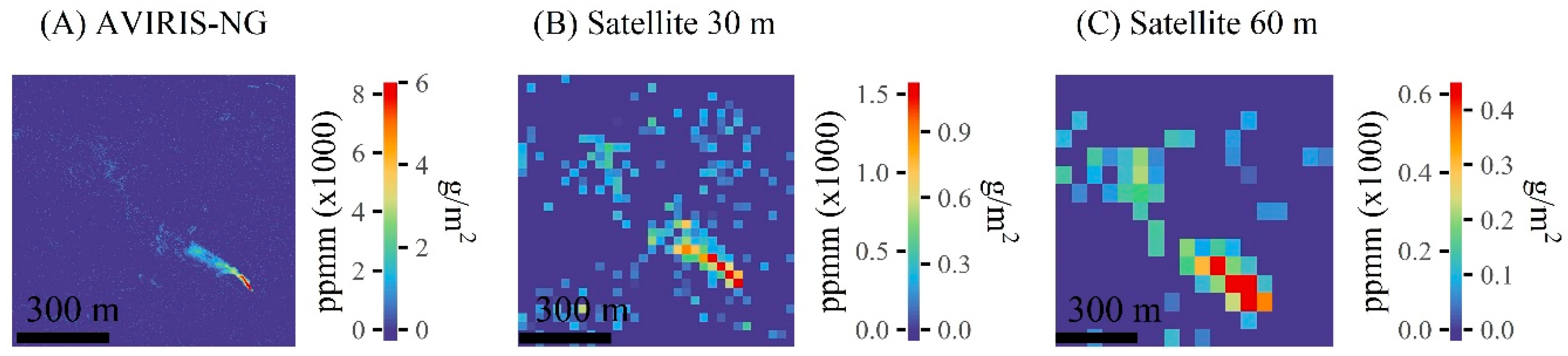
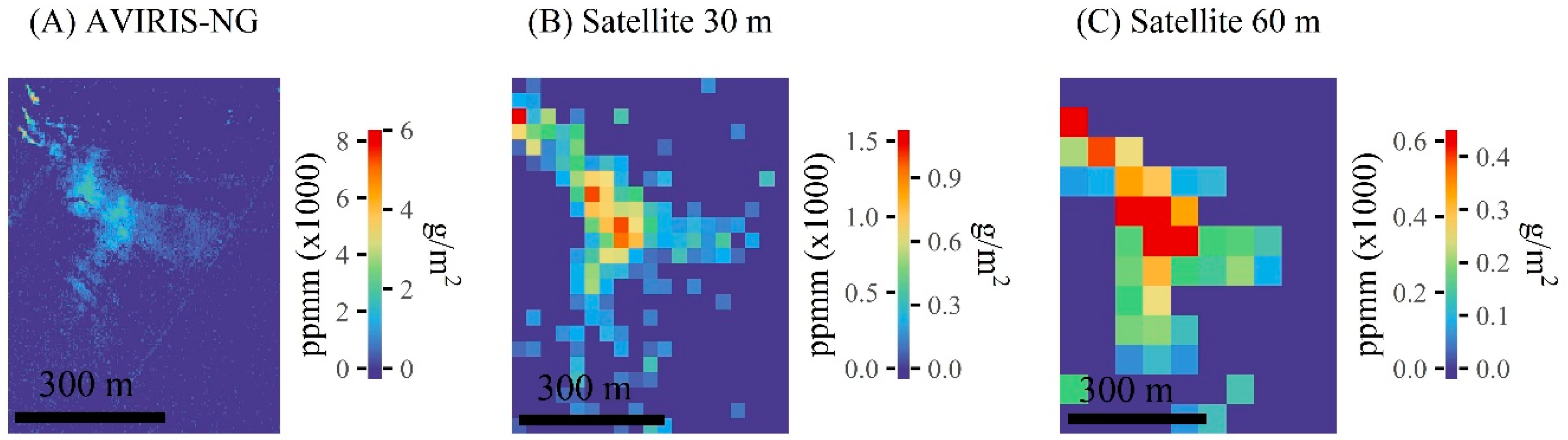
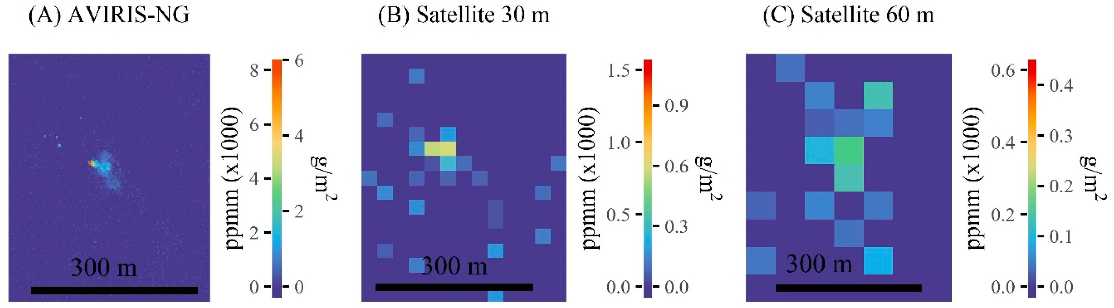
3.1. Methane Plumes by Sector

One advantage of using a satellite system to detect methane plumes is the ability to observe a large diversity of methane emitting sectors. Plumes from different sectors have different shapes, sizes, and underlying land cover that can influence how well a plume is detected. Here, we look at plumes from the three largest anthropogenic methane emitting sectors to understand how well a satellite system would perform in each sector. The following sections present the matched filter methane retrieval results for the AVIRIS-NG, 30 m, and 60 m satellite simulations.

3.1.1. Petroleum and Natural Gas

The natural gas and petroleum industry represents about 30%–35% of all anthropogenic methane emissions globally [2,4,48]. Methane emissions from this sector can be challenging to characterize, given the significant variability in source type, plume shape and size, and intermittence. Here, we present three examples from different sources. The first is a gas storage facility that has two emission sources, the second is a well with a methane plume, and the third is a leak from a natural gas distribution line in a neighborhood [7]. All plumes were detectable from the 30 m and 60 m simulated satellite images.
Figure 3 depicts the results of two plumes at the Honor Ranch gas storage facility. The source for the top plume is an emergency shutdown stack and for the bottom plume, it is a compressor unit. In the AVIRIS-NG image, these two plumes were distinct, which allows the plumes to be attributed to their exact sources. In the 30 m image, some of the detail of the plume is lost, but two distinct plumes are still visible. At 60 m, the methane enhancement is visible, but the distinction between the two plumes disappears. At the 30 m and 60 m resolution, we could easily attribute the plume to the facility, but not to the exact locations within the facility as we could with the original AVIRIS-NG image.
Figure 4 shows the matched filter results from a methane plume from a well. Given the sheer quantity and high density of wells throughout the United States, a satellite system would be well suited to identify those that are emitting methane. This particular example is from a hydrocarbon extraction site within the Aliso Canyon gas storage facility. The details of the plume are most distinct in the original AVIRIS-NG image. In the 30 m and 60 m satellite images, the plume is still clearly detectable, but becomes increasingly less detailed.
One concern in the natural gas and petroleum sector are leaks and other fugitive emissions. Not only do these emissions contribute to the overall greenhouse gas budget, but they also represent lost revenue and in sufficiently large amounts can pose a public safety hazard. The ability to detect leaks over large areas could help improve the mitigation of greenhouse gas emissions and hazards. Figure 5 is an example of an underground natural gas distribution line leak that was detected in 2016 in the Chino Hills neighborhood, CA. This particular leak was detected using the real time methane mapping capability of AVIRIS-NG and the results were shared with the local gas company who quickly confirmed and repaired the leak [19]. The plume is clearly visible in the AVIRIS-NG image and a distinct methane enhancement is visible in the 30 m and 60 m simulated images.
Current and past satellite sensors, like SCIAMACY and TROPOMI, are able to detect regional methane enhancements over areas with heavy oil and gas production, like the methane anomaly over the Four Corners areas in the Western United Sates [49], but cannot identify the exact location of individual point sources. Currently, the only way to locate a specific source is through a ground or airborne campaign, which can be costly, time consuming, and have a limited geographic extent [6]. Therefore, a higher spatial resolution satellite sensor that could identify point sources would help us understand the dynamics of oil and natural gas methane emissions. Other studies have looked into the possibility of using spaceborne sensors to do fine scale methane plume detection. Varon et al. [13] performed a sensitivity study indicating that individual plumes could be mapped with a sufficiently sensitive constellation of point source monitoring satellites, similar to the planned GHGSat fleet. In addition, Cusworth et al. showed that plumes from oil/gas facilities could be detected with the upcoming EnMAP mission [50]. The future generation of imaging spectrometers will help us to improve our understanding of methane emissions from the oil and natural gas sectors.

3.1.2. Landfill/Wastewater Treatment

The waste sector, which includes landfills and wastewater treatment, is thought to make up about 16% of global anthropogenic methane emissions, with the majority coming from landfills [2,4,47]. Globally, landfills take on many different forms, and factors like the composition of the waste, the temperature, the age, and management system can all influence the amount of methane emitted from a landfill [51,52,53]. Of those landfills exhibiting plumes during the California Methane Survey, plumes appeared persistent across multiple years, therefore making them an excellent target for spaceborne studies [7]. Satellite monitoring of these sites can help understand emissions from this under sampled sector, assess gas capture systems, and generally provide a better understanding of landfill emissions.
Figure 6 shows the matched filter results from the Newby Island landfill in San Jose, CA. In this image, a very large plume is present, originating from multiple places in the landfill. Note the scale on (C) Satellite 60 m is higher than the other figures, which is due to the large size of the plume. The plume remains visible in all simulated satellite images. Large plumes have been detected with AVIRIS-NG from other landfills in California and a large landfill in India, indicating that this type of methane source can be studied from space.
Adjacent to the landfill is a wastewater treatment facility. Figure 7 shows a small plume that is evidently emanating from one of the tanks. The plume is clearly visible in the AVIRIS-NG image, but less so in the 30 m and 60 m images. Given this result, the detection of a methane plume from this particular source will be difficult for the satellite instruments modeled here.

3.1.3. Dairies

Enteric fermentation and manure management make up about 28% of global anthropogenic methane emissions [2,4,48]. This is a significant anthropogenic methane source, but the most difficult to map using this method. Enteric fermentation is an area source and does not produce methane from a single easily identifiable point. This makes mapping methane from cattle with imaging spectroscopy more difficult. However, there is an exception for some methods of manure management. Many manure lagoons from large dairies and some digesters in California produce small yet detectable plumes. Figure 8 shows the matched filter results of a plume from a typical dairy manure lagoon. It is clearly visible in the AVIRIS-NG images and remains detectable in the 30 m and 60 m images.
An anaerobic digester is an enclosed area where the breakdown of organic material (manure) is promoted and the biogas is then captured and used as an energy source. Many studies have measured the potential biogas produced from digesters in order to estimate gas production [54,55]. However, few studies have looked at the gas lost due to leaks. In addition, emissions from manure can be well constrained with isotopic measurements, but this does not allow for the distinction between an open manure lagoon and a digester [56]. Regular satellite measurements of large dairy production areas like California’s San Joaquin Valley would improve understanding of the dynamics of methane emission from manure management. Figure 9 shows the matched filter results of three plumes in the upper left corner coming off a digester in California. In the 30 m and 60 m simulated images, the plume is still visible, but has blended into one larger plume instead of three smaller ones.

3.1.4. Controlled Release
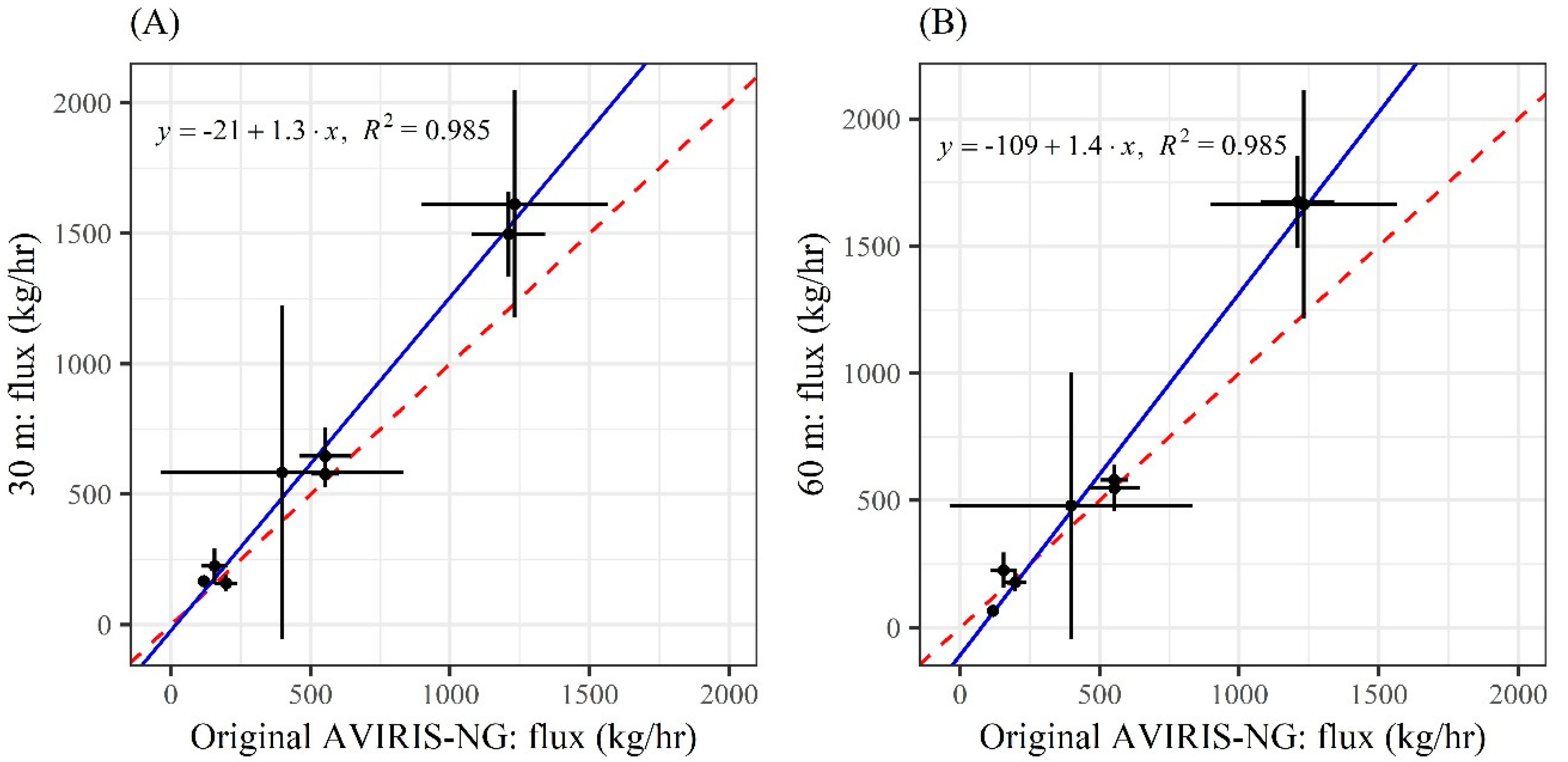
In September 2018, a controlled release experiment was performed to test the accuracy of the AVIRIS-NG methane retrievals. Natural gas was released by a pipeline operator at a known flux while AVIRIS-NG flew over. We analyzed one scene from this experiment to verify that our methods were producing reasonable results (Figure 10). The flux during this flight was 103.71 kg/h and the retrieval from AVIRIS-NG with our methods was 117.59 ± 15.53 kg/h. The agreement between the AVIRIS-NG flux and actual flux was good, however, the agreement for the 30 m and 60 m images was not as close (Table 2). This was a smaller plume and the entire plume spanned one or two pixels in the 60 m satellite simulation, therefore calculating an accurate flux was more difficult. Regardless, the plumes were visible in both the 30 m and 60 m, which indicates that plumes with a flux as small as ~100 kg/h will be visible with the next generation of satellite imaging spectrometers.

3.2. Flux

The fluxes for the AVIRIS-NG, 30 m, and 60 m images were calculated using the methods presented above. Calculating the flux allows the scientific community to quantitatively assess the volume of methane emitted per source and sector. We tested an image from a controlled release experiment (presented above) to empirically validate our flux estimates. We calculated a flux estimation of 117.59 ± 15.53 kg/h for the AVIRIS-NG image of the controlled release experiment. The reported flux at the time of the image was 103.71 kg/h. These results are close enough that we feel confident that the AVIRIS-NG images provide a good estimation of the magnitude of the flux. We can therefore compare the results from the satellite simulations to the original AVIRIS-NG image to understand how well a satellite system would perform. In general, the flux estimates from the satellite simulations are consistent with the flux estimations from the AVIRIS-NG image. Table 2 provides the results of the flux estimates for the AVIRIS-NG, the 30 m, and 60 m images. Figure 11 shows the flux results from the 30 m and 60 m image plotted against the flux results from the AVIRIS-NG image. The relationship between the satellite simulations and the AVIRIS-NG image was strong (R2 = 0.98), although the linear regression line did not match the 1:1 line, the error bars crossed or came close to the 1:1 line. The satellite simulations tended to overestimate the flux for both simulations. In addition, the overestimation appears to become larger as the size of the methane plume increases, however, when the error is normalized by the size of the plume, this relationship breaks down. One explanation for the overestimation is that the coarser spatial resolution inflates the spatial extent of the plume, which increases the IME and plume length. However, the IME tends to increase more than the plume length, causing the flux to also increase. In a similar study, Cusworth et al. found that the satellite simulation underestimated the AVIRIS-NG retrieval, but they used a different retrieval algorithm, a different plume mask, and did not simulate a 60 m instrument [50]. More work will be needed to be done to understand precisely how increasing spatial resolution changes the IME and therefore the flux.

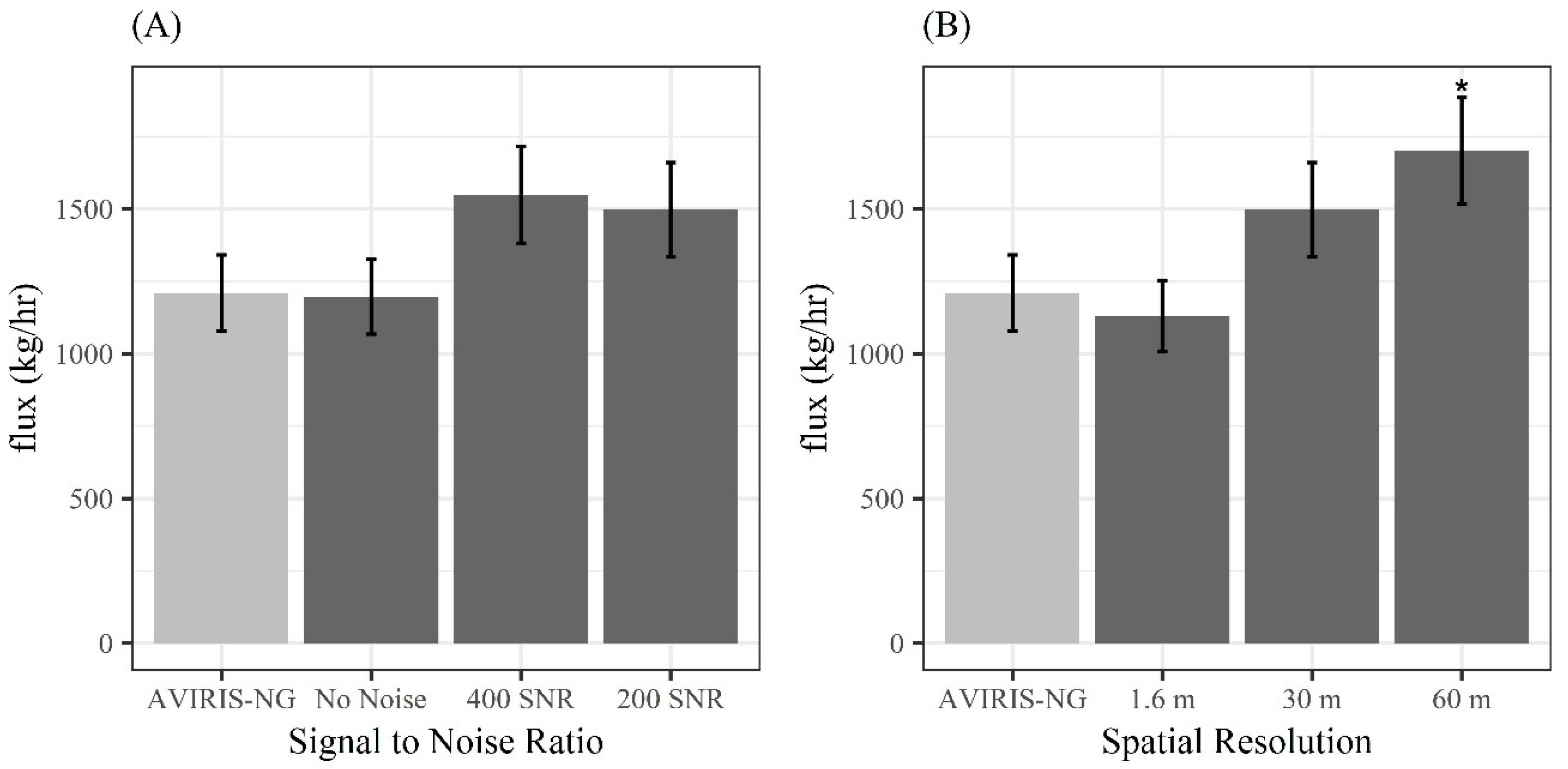
3.3. Spatial Resolution and Signal-to Noise Ratio

In this analysis, the spatial resolution and SNR are the two variables that distinguish the 30 m and 60 m satellite simulations. Sensor design often requires compromises between different performance measures. For example, designers may sacrifice SNR for finer spatial resolution and vice versa. We looked at which of these factors had the largest impact on methane gas mapping. We used the Honor Ranch gas storage facility as an example and tested how our retrieval changed with different noise levels; no added noise, ~400 SNR, and ~200 SNR. We found that visually, the plume became less distinct from the background and the presence of spurious signals increased, which in turn slightly increased the flux estimate (Figure 12). We also tested the image with the same SNR at the native resolution (1.6 m), 30 m, and 60 m. We found that the plume became less detailed with coarsening spatial resolution, indicating that spatial resolution, rather than SNR, had a larger influence on detecting plumes. In addition, we performed an Analysis of Variance (ANOVA) with a Tukey post hoc using the flux and standard deviation, and found that the only image that was significantly different (p ≤ 0.05) from the original AVIRIS-NG was the 60 m image. More plumes as well as a larger range in SNR and pixel size will be needed to accurately quantify how noise versus spatial resolution effects plume retrieval. However, these results indicate that changing the spatial resolution has a larger impact than changing the noise.

3.4. Limitations

The satellite simulations indicate that point source methane mapping will be possible with the future generation of satellite imaging spectrometers. However, there are some limitations with the simulations presented here. While the specifications for the simulation represent the best available knowledge about the design of a future spectrometer (EMIT), there remains a possibility that specifications will change before launch. Other satellite designs might include different spectral, spatial, or SNR characteristics not modeled here, however these are unlikely to be drastically different. In addition, this study did not account for other factors associated with satellite sensors including potential orbits, cloud cover, sun angles, and surface brightness. In particular, surface brightness has proven to have a large influence on methane retrievals [50,57]. While there is inherent variability in surface brightness in the AVIRIS-NG scenes, we were not able to control this variable. Finally, while the flightlines from this study represent a range of emissions over variable surface terrain, more challenging examples containing lower fluxes were not tested.
Other limitations in the study include the methods we used to create a plume mask and the flux estimate. The plume mask is intended to isolate the plume and filter out spurious signals or false positives. Spurious signals were present in both the airborne data and the satellite simulations (Figure 3, Figure 4, Figure 5, Figure 6, Figure 7, Figure 8, Figure 9 and Figure 10). For this study, we attempted to be as consistent as possible and therefore generally used consistent thresholds to isolate the plume. It should be noted, however, that more tailored thresholding could produce better results in future studies. The thresholding and segmentation can have a large impact on the results, more work is needed to determine the best practices for how to approach this. Additional work is required to assess the impact that these spurious signals may have on our IME and flux estimates. This study also used a simple method to estimate the flux of the plumes. More robust flux calculations could lead to more accurate results.

4. Conclusions

We tested the potential to use future Earth observing satellites such as EMIT or SBG to map and measure methane plumes from the three main anthropogenic emission sectors. These particular future satellites will measure in the SWIR with 7–10 nm spectral sampling, the spatial resolution will range from 30 m to 60 m pixels, and will have a SNR in the SWIR between 200 and 400. To test the potential of using these instruments for high resolution methane mapping, we simulated two proposed satellite designs from the AVIRIS-NG data. The first was a 30 m pixel resolution with a ~200 SNR in the SWIR, the second was a 60 m pixel resolution with ~400 SNR in the SWIR. We then ran a matched filter methane retrieval algorithm on the simulated satellite images and compared it to the original AVIRIS-NG.
We found that for almost all plumes, the methane enhancement remained visible at the coarser spatial resolutions. This indicated that most point source emissions from the largest anthropogenic sources should be detectable, at minimum, in a 30 m resolution image. We found that when we quantified the flux of the plume in the simulated images, it correlated well with the flux calculated from the AVIRIS-NG results. In addition, for the controlled release experiment, the flux calculated from the AVIRIS-NG data was similar to the known flux. Within the limits of our study, we also found that the spatial resolution had a larger impact on the results than the SNR. We conclude that a satellite system will be able to map and quantify the biggest of the point source emitters and should be able to detect plumes as small as ~100 kg/h, although accurate quantification of flux may be more difficult. These plumes may only be a small fraction of the total number of plumes, but likely represent up to 40% of emitted methane.
While the future generation of satellite imaging spectrometers were not designed for high resolution gas mapping, this work indicates that they will be able to map methane plumes and quantify emission rates. However, imaging spectrometer concepts have been developed that would utilize finer spectral resolution to improve gas sensitivities [50,58]. Eventually, these sensors will become integrated into larger greenhouse gas monitoring schemes and will help scientists better understand global methane emissions.

Author Contributions

A.K.A. created the model, performed the analysis, and was the main author. P.E.D., D.A.R., and A.K.T. helped conceive the experimental design and methodological approach. M.F., P.E.D., and S.J. developed and assisted with the methane retrieval algorithm. A.K.T. and R.M.D. provided the AVIRIS-NG data and contributed supporting material. R.O.G. and D.R.T. provided information on the design for the satellite simulations.

Funding

This research was funded by the National Aeronautics and Space Administration (NASA), grant number 80NSSC17K0575.

Acknowledgments

A portion of this research was supported by the Chevron Energy Technology Company and performed at the Jet Propulsion Laboratory, California Institute of Technology, under contract with the National Aeronautics and Space Administration (NASA). US Government support is acknowledged. Data for this research was provided by the California Methane Survey funded by NASA, the California Air Resources Board, the California Energy Commission, and NASA’s Carbon Monitoring System.

Conflicts of Interest

The authors declare no conflicts of interest.

Appendix A

Table A1. MODerate resolution atmospheric TRANsmission (MODTRAN) inputs for simulating the atmosphere from the aircraft to the top-of-atmosphere (TOA).
AttributeValues
Wavelengths350–2500 nm
Carbon dioxide405 ppm
Water Vapor1245.3 atm-cm
Visibility30 km
Methane1.7 ppm
Figure A1. Example a radiance spectrum for the original AVIRIS-NG (red) and example of the same spectrum adjusted for TOA (blue).
Remotesensing 11 03054 g0a1
Figure A2. Example of a radiance spectrum at 5 nm sampling (blue) and the same example at 7.5 nm sampling (red). Note the decreased detail in the gas absorption bands.
Remotesensing 11 03054 g0a2
Table A2. Integrated Mass Enhancements (IME) and lengths for all plumes.
SourceIME (kg)Length (m)
AVIRIS-NG30 m60 mAVIRIS-NG30 m60 m
Gas Storage Facility70.23116.51128.23671.50900.00885.89
Well ***13.3028.6014.63314.87550.73349.86
Gas Distribution Line6.9911.5414.51224.79258.07323.11
Landfill *325.73442.21469.162123.182200.662264.16
Wastewater Treatment 5.542.023.22208.9794.87134.16
Dairy Manure Lagoon **12.519.7810.05360.80192.09240.00
Dairy Digester23.9628.6024.40483.04550.73468.62
Controlled Release1.621.590.5897.7167.0862.92
* 600 pixel threshold for the AVIRIS-NG image, eight pixels for the 30 m, and four for the 60 m; ** 2000 pixel threshold for the AVIRIS-NG image, 15 pixels for the 30 m, and four for the 60 m; *** 25 pixel threshold for the 30 m image and four pixels for the 60 m; A 300 ppm-m threshold was used for the 30 m and 60 m images.
Table A3. Mean wind speed and standard deviation for each plume from the High-Resolution Rapid Refresh (HRRR) reanalysis product.
SourceMean Wind Speed (m/s)Standard Deviation Wind Speed (m/s)
Gas Storage Facility1.3950.430
Pump Jack3.2130.348
Pipeline Leak3.1873.479
Landfill3.0940.267
Wastewater Treatment2.0750.423
Dairy Manure Lagoon2.2300.602
Dairy Digester3.6370.610
Controlled Release1.9590.258

References

  1. Ciais, P.; Sabine, C.; Bala, G.; Bopp, L.; Brovkin, V.; Canadell, J.; Chhabra, A.; DeFries, R.; Galloway, J.; Heimann, M.; et al. “Carbon and Other Biogeochemical Cycles.”. In Climate Change 2013 – The Physical Science Basis: Working Group I Contribution to the Fifth Assessment Report of the Intergovernmental Panel on Climate Change; Cambridge University Press: Cambridge, UK, 2014; pp. 465–570. [Google Scholar] [CrossRef] [Green Version]
  2. Saunois, M.; Bousquet, P.; Poulter, B.; Peregon, A.; Ciais, P.; Canadell, J.G.; Janssens-Maenhout, G.; Giuseppe, E.; David, B.; Houweling, S.; et al. The global methane budget 2000–2012. Earth Syst. Sci. Data 2016, 8, 697–751. [Google Scholar] [CrossRef] [Green Version]
  3. Kirschke, S.; Bousquet, P.; Ciais, P.; Saunois, M.; Canadell, J.G.; Dlugokencky, E.J.; Bergamaschi, P.; Bergmann, D.; Blake, D.R.; Bruhwiler, L.; et al. Three decades of global methane sources and sinks. Nat. Geosci. 2013, 6, 813–823. [Google Scholar] [CrossRef]
  4. Inventory of US Greenhouse Gas Emissions and Sinks: 1990–2014; U.S. Environmental Protection Agency: Washington, DC, USA, 2016.
  5. Allen, D.T.; Pacsi, A.P.; Sullivan, D.W.; Zavala-araiza, D.; Harrison, M.; Keen, K.; Fraser, M.P.; Hill, A.D.; Sawyer, R.F.; Seinfeld, J.H. Methane Emissions from Process Equipment at Natural Gas Production Sites in the United States: Pneumatic Controllers. Environ. Sci. Technol. 2015, 49, 641–648. [Google Scholar] [CrossRef] [PubMed]
  6. Frankenberg, C.; Thorpe, A.K.; Thompson, D.R.; Hulley, G.; Kort, E.A.; Vance, N.; Borchardt, J.; Krings, T.; Gerilowski, K.; Sweeney, C.; et al. Airborne methane remote measurements reveal heavy-tail flux distribution in Four Corners region. Proc. Natl. Acad. Sci. USA 2016, 113, 9734–9739. [Google Scholar] [CrossRef] [PubMed] [Green Version]
  7. Duren, R.M.; Thorpe, A.K.; Foster, K.T.; Rafiq, T.; Hopkins, F.M.; Yadav, V.; Bue, B.D.; Thompson, D.R.; Conley, S.; Colombi, N.; et al. California’s Methane Super-Emitters. Nature 2019, 575, 180–184. [Google Scholar] [CrossRef] [Green Version]
  8. Hu, H.; Aben, I.; Landgraf, J.; Detmers, R.; Borsdorff, T.; Butz, A. Toward Global Mapping of Methane With TROPOMI: First Results and Intersatellite Comparison to GOSAT. Geophys. Res. Lett. 2018, 45, 3682–3689. [Google Scholar] [CrossRef]
  9. Xiong, X.; Barnet, C.; Maddy, E.; Sweeney, C.; Liu, X.; Zhou, L.; Goldberg, M. Characterization and validation of methane products from the Atmospheric Infrared Sounder (AIRS). J. Geophys. Res. Biogeosci. 2008, 113, 1–14. [Google Scholar] [CrossRef]
  10. Frankenberg, C.; Meirink, J.F.; van Weele, M.; Platt, U.; Wagner, T. Assessing Methane Emissions from Global Space-Borne Observations. Science 2005, 308, 1010–1014. [Google Scholar] [CrossRef] [Green Version]
  11. Turner, A.J.; Frankenberg, C.; Wennberg, P.O.; Jacob, D.J. Ambiguity in the causes for decadal trends in atmospheric methane and hydroxyl. Proc. Natl. Acad. Sci. 2017, 114, 5367–5372. [Google Scholar] [CrossRef] [Green Version]
  12. Cusworth, D.H.; Jacob, D.J.; Sheng, J.; Benmergui, J.; Turner, A.J.; Brandman, J.; White, L.; Randles, C.A. Detecting high-emitting methane sources in oil/gas fields using satellite observations. Atmos. Chem. Phys. 2018, 16885–16896. [Google Scholar] [CrossRef] [Green Version]
  13. Varon, D.J.; Jacob, D.J.; Mckeever, J.; Jervis, D.; Durak, B.O.A.; Xia, Y. Quantifying methane point sources from fine-scale ( GHGSat ) satellite observations of atmospheric methane plumes. Atmos. Meas. Tech. 2018, 11, 5673–5686. [Google Scholar] [CrossRef] [Green Version]
  14. Varon, D.J.; Mckeever, J.; Jervis, D.; Maasakkers, J.D.; Pandey, S.; Houweling, S. Satellite discovery of anomalously large methane point sources from oil/gas production. Geophys. Res. Lett. 2019. [Google Scholar] [CrossRef] [Green Version]
  15. Rast, M.; Painter, T.H. Earth Observation Imaging Spectroscopy for Terrestrial Systems: An Overview of Its History, Techniques, and Applications of Its Missions. Surv. Geophys. 2019, 40, 303–331. [Google Scholar] [CrossRef]
  16. Roberts, D.A.; Bradley, E.S.; Cheung, R.; Leifer, I.; Dennison, P.E.; Margolis, J.S. Mapping methane emissions from a marine geological seep source using imaging spectrometry. Remote Sens. Environ. 2010, 114, 592–606. [Google Scholar] [CrossRef]
  17. Thorpe, A.K.; Roberts, D.A.; Bradley, E.S.; Funk, C.C.; Dennison, P.E.; Leifer, I. High resolution mapping of methane emissions from marine and terrestrial sources using a Cluster-Tuned Matched Filter technique and imaging spectrometry. Remote Sens. Environ. 2013, 134, 305–318. [Google Scholar] [CrossRef]
  18. Thorpe, A.K.; Frankenberg, C.; Thompson, D.R.; Duren, R.M.; Aubrey, A.D.; Bue, B.; Green, R.O.; Gerilowski, K.; Krings, T.; Borchard, J.; et al. Airborne retrievals of methane, carbon dioxide, and water vapor concentrations at high spatial resolution: application to AVIRIS-NG. Atmos. Meas. Tech. 2017, 10, 3833–3850. [Google Scholar] [CrossRef] [Green Version]
  19. Thompson, D.R.; Leifer, I.; Bovensmann, H.; Eastwood, M.; Fladeland, M.; Frankenberg, C.; Gerilowski, K. Real-time remote detection and measurement for airborne imaging spectroscopy: a case study with methane. Atmos. Meas. Tech. 2015, 8, 4383–4397. [Google Scholar] [CrossRef] [Green Version]
  20. Bradley, E.S.; Leifer, I.; Roberts, D.A.; Dennison, P.E.; Washburn, L. Detection of marine methane emissions with AVIRIS band ratios. Geophys. Res. Lett. 2011, 38. [Google Scholar] [CrossRef]
  21. Gao, B.-C.; Goetz, A.F.H. Column atmospheric water vapor and vegetation liquid water retrievals from Airborne Imaging Spectrometer data. J. Geophys. Res. 1990, 95, 3549. [Google Scholar] [CrossRef]
  22. Thorpe, A.K.; Roberts, D.A.; Dennison, P.E.; Bradley, E.S.; Funk, C.C. Point source emissions mapping using the Airborne Visible/Infrared Imaging Spectrometer (AVIRIS). In Proceedings of the SPIE Proceedings-Algorithms Technol. Multispectral, Hyperspectral, Ultraspectral Imag. XVIII, Baltimore, MD, USA, 15 May 2012. [Google Scholar] [CrossRef]
  23. Stefano, P.; Angelo, P.; Simone, P.; Filomena, R.; Federico, S.; Umberto, A.; Vincenzo, C.; Roberto, D.B.; Giovanni, L.; La, R.; et al. The PRISMA hyperspectral mission: science activities and opportunities for agriculture and land monitoring. In Proceedings of the 2013 IEEE International Geoscience and Remote Sensing Symposium(IGARSS), Melbourne, VIC, Australia, 21–26 July 2013; pp. 4558–4561. [Google Scholar]
  24. Loizzo, R.; Guarini, R.; Longo, F.; Scopa, T.; Formaro, R.; Facchinetti, C.; Varacalli, G. PRISMA: THE Italian hyperspectral mission. In Proceedings of the 2018 IEEE International Geoscience and Remote Sensing Symposium, Valencia, Spain, 22–27 July 2018; pp. 175–178. [Google Scholar]
  25. Guanter, L.; Kaufmann, H.; Segl, K.; Foerster, S.; Rogass, C.; Chbrillat, S.; Fischer, S.; Schrader, S.; Storch, T.; Heiden, U.; et al. The EnMAP Spaceborne Imaging Spectroscopy Mission for Earth Observation. Remote Sens. 2015, 7, 8830–8857. [Google Scholar] [CrossRef] [Green Version]
  26. Matsunaga, T.; Iwasaki, A.; Tsuchida, S.; Iwao, K.; Tanii, J.; Kashimura, O.; Nakamurac, R.; Yamamotoc, H.; Katoc, S.; Obatac, K.; et al. Hisui Status Toward Fy2019 Launch. IEEE Int. Geosci. Remote Sens. Symp. 2018, 160–163. [Google Scholar]
  27. Thriving on Our Changing Planet: A Decadal Strategy for Earth Observation from Space; National Academies of Sciences Engineering and Medicine: Washington, DC, USA, 2018; ISBN 9780309467575.
  28. Thompson, D.R.; Thorpe, A.K.; Frankenberg, C.; Green, R.O.; Duren, R.; Guanter, L.; Hollstein, A.; Middleton, E.; Ong, L.; Ungar, S. Space-based Remote Imaging Spectroscopy of the Aliso Canyon CH4 Super-emitter. Geophys. Res. Lett. 2016, 43, 6571–6578. [Google Scholar] [CrossRef] [Green Version]
  29. Green, R.O.; Mahowald, N.M.; Clark, R.N.; Ehlmann, B.L.; Ginoux, P.A.; Kalashnikova, O.V.; Miller, R.L.; Okin, G.; Painter, T.H.; Pérez García-Pando, C.; et al. NASA’s Earth Surface Mineral Dust Source Investigation. Proceedings of AGU Fall Meeting 2018, Washington, DC, USA, 10–14 December 2018. [Google Scholar]
  30. Hamlin, L.; Green, R.O.; Mouroulis, P.; Eastwood, M.; Wilson, D.; Dudik, M.; Paine, C. Imaging spectrometer science measurements for terrestrial ecology: AVIRIS and new developments. In Proceedings of the 2011 Aerospace Conference, Big Sky, MT, USA, 5–12 March 2011; 2011; pp. 1–7. [Google Scholar]
  31. Green, R.O.; Eastwood, M.L.; Sarture, C.M.; Chrien, T.G.; Aronsson, M.; Chippendale, B.J.; Faust, J.A.; Pavri, B.E.; Chovit, C.J.; Solis, M.; et al. Imaging spectroscopy and the Airborne Visible/Infrared Imaging Spectrometer (AVIRIS). Remote Sens. Environ. 1998, 65, 227–248. [Google Scholar] [CrossRef]
  32. Chapman, J.W.; Thompson, D.R.; Helmlinger, M.C.; Bue, B.D.; Green, R.O.; Eastwood, M.L.; Geier, S.; Olson-duvall, W.; Lundeen, S.R. Spectral and Radiometric Calibration of the Next Generation Airborne Visible Infrared Spectrometer (AVIRIS-NG). Remote Sens. 2019, 11, 2129. [Google Scholar] [CrossRef] [Green Version]
  33. Duren, R.; Thorpe, A.; Sander, S. California Baseline Methane Survey-Interim Phase 1 report. In Proceedings of the 2017 AGU Fall Meeting, New Orleans, LA, USA, 11–15 December 2017. [Google Scholar]
  34. Berk, A.; Conforti, P.; Kennett, R.; Perkins, T.; Hawes, F.; Van Den Bosch, J. MODTRAN® 6: A major upgrade of the MODTRAN® radiative transfer code. In Proceedings of the 2014 6th Workshop on Hyperspectral Image and Signal Processing: Evolution in Remote Sensing (WHISPERS), Lausanne, Switzerland, 24–27 June 2014. [Google Scholar]
  35. Funk, C.C.; Theiler, J.; Roberts, D.A.; Borel, C.C. Clustering to improve matched filter detection of weak gas plumes in hyperspectral thermal imagery. IEEE Trans. Geosci. Remote Sens. 2001, 39, 1410–1420. [Google Scholar] [CrossRef] [Green Version]
  36. Theiler, J.; Foy, B.R. Effect of signal contamination in matched-filter detection of the signal on a cluttered background. IEEE Geosci. Remote Sens. Lett. 2006, 3, 98–102. [Google Scholar] [CrossRef]
  37. Manolakis, D.; Lockwood, R.; Cooley, T.; Jacobson, J. Robust Matched Filters for Target Detection in Hyperspectral Imaging Data. In Proceedings of the 2007 IEEE International Conference on Acoustics, Speech and Signal Processing - ICASSP ’07, Honolulu, HI, USA, 15–20 April 2007. [Google Scholar]
  38. Donoho, D.L. Compressed sensing. IEEE Trans. Inf. Theory 2006, 52, 1289–1306. [Google Scholar] [CrossRef]
  39. Candès, E. Compressive sampling. In Proceedings of the International Congress of Mathematicians, Madrid, Spain, 22–30 August 2006; pp. 1433–1452. [Google Scholar]
  40. Lustig, M.; Donoho, D.; Pauly, J.M. Sparse MRI: The application of compressed sensing for rapid MR imaging. Magn. Reson. Med. 2007, 58, 1182–1195. [Google Scholar] [CrossRef]
  41. Wiaux, Y.; Jacques, L.; Puy, G.; Scaife, A.M.M.; Vandergheynst, P. Compressed sensing imaging techniques for radio interferometry. Mon. Not. R. Astron. Soc. 2009, 395, 1733–1742. [Google Scholar] [CrossRef]
  42. Stevens, A.; Kovarik, L.; Abellan, P.; Yuan, X.; Carin, L.; Browning, N.D. Applying compressive sensing to TEM video: a substantial frame rate increase on any camera. Adv. Struct. Chem. Imaging 2015, 1, 10. [Google Scholar] [CrossRef] [Green Version]
  43. Beck, A.; Teboulle, M. A Fast Iterative Shrinkage-Thresholding Algorithm for Linear Inverse Problems. SIAM J. Imaging Sci. 2009, 2, 183–202. [Google Scholar] [CrossRef] [Green Version]
  44. Theiler, J.; Foy, B.R.; Fraser, A.M. Nonlinear signal contamination effects for gaseous plume detection in hyperspectral imagery. In Proceedings of the Defense and Security Symposium, Orlando, FL, USA, 17–21 April 2006. [Google Scholar]
  45. Foote, M.; Dennison, P.; Thorpe, A.; Thompson, D.; Jongaramrungruang, S.; Frankenberg, C.; Joshi, S. Fast and Accurate Retrieval of Methane Concentration from Imaging Spectrometer Data Usinf Sparsity Prior. IEEE TGRS. in press.
  46. Blaylock, B.K.; Horel, J.D.; Liston, S.T. Computers and Geosciences Cloud archiving and data mining of High-Resolution Rapid Refresh forecast model output. Comput. Geosci. 2017, 109, 43–50. [Google Scholar] [CrossRef]
  47. Horel, J.; Blaylock, B. Archive of the High Resolution Rapid Refresh model. Available online: https://hive.utah.edu/concern/datasets/47429912h (accessed on 6 January 2019).
  48. EPA. Global Mitigation of Non-CO 2 Greenhouse Gases: 2010–2030. 2013. Available online: https://www.epa.gov/sites/production/files/2016-06/documents/mac_report_2013.pdf (accessed on 1 February 2017).
  49. Kort, E.A.; Frankenberg, C.; Costigan, K.R.; Lindenmaier, R.; Dubey, M.K.; Wunch, D. Four corners: The largest US methane anomaly viewed from space. Geophys. Res. Lett. 2014, 41, 6898–6903. [Google Scholar] [CrossRef]
  50. Cusworth, D.H.; Jacob, D.J.; Varon, D.J.; Miller, C.C.; Liu, X.; Chance, K. Potential of next-generation imaging spectrometers to detect and quantify methane point sources from space. Atmos. Meas. Tech. 2019, 12, 5655–5668. [Google Scholar] [CrossRef] [Green Version]
  51. Bingemer, H.G.; Crutzen, P.J. The production of methane from solid wastes. J. Geophys. Res. 1987, 92, 2181. [Google Scholar] [CrossRef] [Green Version]
  52. Themelis, N.J.; Ulloa, P.A. Methane generation in landfills. Renew. Energy 2007, 32, 1243–1257. [Google Scholar] [CrossRef]
  53. Goldsmith, C.D.; Chanton, J.; Abichou, T.; Swan, N.; Green, R.; Hater, G. Methane emissions from 20 landfills across the United States using vertical radial plume mapping. J. Air Waste Manage. Assoc. 2012, 62, 183–197. [Google Scholar] [CrossRef] [Green Version]
  54. Jiang, Y.; Banks, C.; Zhang, Y.; Heaven, S.; Longhurst, P. Quantifying the percentage of methane formation via acetoclastic and syntrophic acetate oxidation pathways in anaerobic digesters. Waste Manag. 2018, 71, 749–756. [Google Scholar] [CrossRef] [PubMed]
  55. Westerholm, M.; Moestedt, J.; Schnürer, A. Biogas production through syntrophic acetate oxidation and deliberate operating strategies for improved digester performance. Appl. Energy 2016, 179, 124–135. [Google Scholar] [CrossRef] [Green Version]
  56. Townsend-Small, A.; Tyler, S.C.; Pataki, D.E.; Xu, X.; Christensen, L.E. Isotopic measurements of atmospheric methane in Los Angeles, California, USA: Influence of “fugitive” fossil fuel emissions. J. Geophys. Res. Atmos. 2012, 117, 1–11. [Google Scholar] [CrossRef]
  57. Ayasse, A.K.; Thorpe, A.K.; Roberts, D.A.; Frankenberg, C.; Aubrey, A.D.; Dennison, P.E.; Funk, C.C.; Teffke, A. Evaluating the effects of surface properties on methane retrievals using a synthetic airborne visible/infrared imaging spectrometer next generation (AVIRIS-NG) image. Remote Sens. Environ. 2018, 215, 386–397. [Google Scholar] [CrossRef]
  58. Thorpe, A.K.; Frankenberg, C.; Green, R.O.; David, R.; Aubrey, A.D.; Mouroulis, P.; Eastwood, M.L. The Airborne Methane Plume Spectrometer ( AMPS ): Quantitative Imaging of Methane Plumes in Real Time. In Proceedings of the IEEE Aerospace Conference, Big Sky, MT, USA, 5–12 March 2016. [Google Scholar]
Figure 1. Flow chart of the steps for creating the simulated satellite data.
Remotesensing 11 03054 g001
Figure 2. Signal-to-Noise Ratio (SNR) for the 30 m simulated satellite data (blue) and for the 60 m simulated satellite data (red).
Remotesensing 11 03054 g002
Figure 3. Matched filter methane retrieval for a plume from a 4 November, 2016 AVIRIS-NG image. The plume is from the Honor Ranch gas storage facility, where there are two plumes, one from an emergency shutdown stack and the other from a compressor unit. (A) Results from the original AVIRIS-NG image. (B) Results from the 30 m simulated satellite image with ~200 SNR. (C) Results from the 60 m simulated satellite image with about ~400 SNR. The left side of the scale bar are units in parts per million per meter (ppm-m) above the background. The right side of the scale bar are methane units in g/m2.
Remotesensing 11 03054 g003
Figure 4. Matched filter methane retrieval results from a plume from a 18 September, 2017 AVIRIS-NG image. The plume is from an oil producing well in Aliso Canyon. (A) Results from the original AVIRIS-NG image. (B) Results from the 30 m simulated satellite image with ~200 SNR. (C) Results from the 60 m simulated satellite image with about ~400 SNR. The left side of the scale bar are units in parts per million per meter (ppm-m) above the background. The right side of the scale bar are methane units in g/m2.
Remotesensing 11 03054 g004
Figure 5. Matched filter methane retrieval results for a plume from a 15 September, 2016 AVIRIS-NG image. The plume is from a low pressure natural gas distribution line leak in the Chino Hills neighborhood. (A) Results from the original AVIRIS-NG image. (B) Results from the 30 m simulated satellite image with ~200 SNR. (C) Results from the 60 m simulated satellite image with about ~400 SNR. The left side of the scale bar are units in parts per million per meter (ppm-m) above the background. The right side of the scale bar are methane units in g/m2.
Remotesensing 11 03054 g005
Figure 6. Matched filter methane retrieval results for a plume from a 18 June, 2017 AVIRIS-NG image. The plume is from Newby Island Land fill in San Jose, CA. (A) Results from the original AVIRIS-NG image. (B) The matched filter results from the 30 m simulated satellite image with ~200 SNR. (C) Results from the 60 m simulated satellite image with about ~400 SNR. The left side of the scale bar are units in parts per million per meter (ppm-m) above the background. The right side of the scale bar are methane units in g/m2.
Remotesensing 11 03054 g006
Figure 7. Matched filter methane retrieval results for a plume from a 18 Jun, 2017 AVIRIS-NG image. The plume a wastewater treatment plant south of the Newby Island Landfill. (A) The matched filter results from the original AVIRIS-NG image. (B) Results from the 30 m simulated satellite image with ~200 SNR. (C) Results from the 60 m simulated satellite image with about ~400 SNR. The left side of the scale bar are units in parts per million per meter (ppm-m) above the background. The right side of the scale bar are methane units in g/m2.
Remotesensing 11 03054 g007
Figure 8. Matched filter methane retrieval results for a plume from a 16 June, 2017 AVIRIS-NG image. The plume is from a typical manure lagoon on a California dairy. (A) The matched filter results from the original AVIRIS-NG image. (B) The matched filter results from the 30 m simulated satellite image with ~200 SNR. (C) The matched filter results from the 60 m simulated satellite image with about ~400 SNR. The left side of the scale bar are units in parts per million per meter (ppm-m) above the background. The right side of the scale bar are methane units in g/m2.
Remotesensing 11 03054 g008
Figure 9. Matched filter methane retrieval results of a plume from a 16 June, 2017 AVIRIS-NG image. The plume is from a covered lagoon digester in California. (A) The matched filter results from the original AVIRIS-NG image. (B) The matched filter results from the 30 m simulated satellite image with ~200 SNR. (C) The matched filter results from the 60 m simulated satellite image with about ~400 SNR. The left side of the scale bar are units in parts per million per meter (ppm-m) above the background. The right side of the scale bar are methane units in g/m2.
Remotesensing 11 03054 g009
Figure 10. Matched filter methane retrieval results from a controlled release experiment on 17 September, 2018. (A) The matched filter results from the original AVIRIS-NG image. (B) The matched filter results from the 30 m simulated satellite image with ~200 SNR. (C) The matched filter results from the 60 m simulated satellite image with about ~400 SNR. The left side of the scale bar are units in parts per million per meter (ppm-m) above the background. The right side of the scale bar are methane units in g/m2.
Remotesensing 11 03054 g010
Figure 11. (A) The 30 m flux plotted against the original AVIRIS-NG. The error bars represent uncertainty in the wind speed estimate, which in turn leads to uncertainty in the flux estimate. The R2 = 0.98, the slope = 1.3, and the y-intercept = −21. (B) The 60 m flux is plotted against the original AVIRIS-NG. The errors bars represent error due to wind speed. The R2 = 0.98, the slope = 1.4, and the y-intercept = −109. For both figures, the red dashed line is the one-to-one line and the blue line is the best fit linear regression.
Remotesensing 11 03054 g011
Figure 12. (A) The y-axis is the flux in kg/h and each bar on the x-axis represents an image. The spatial resolution is held constant (30 m) but the SNR varies from no additional noise, ~400 SNR in the SWIR, and ~200 SNR in the SWIR. (B) The y-axis is the flux (kg/h) and the bars on the x-axis represent images where the SNR is constant (200 SNR) but the spatial resolution is the native 1.6 m, 30 m, and 60 m. The 60 m image is the only image that is significantly different from the AVIRIS-NG, p = 0.019. The light gray bar in both charts is the original AVIRIS-NG for reference and the error bars represent the flux error due to wind speed uncertainty.
Remotesensing 11 03054 g012
Table 1. The Airborne Visible and Infrared Imaging Spectrometers Next Generation (AVIRIS-NG) flight lines used in this study. The methane source type, time, date, and spatial resolution of each flight line.
Line NameSource TypeDate of FlightTime of Flight (UTC)Spatial Resolution
ang20161104t183025Gas Storage Facility11/4/201618:30:251.6 m
ang20160915t185210Gas Distribution Line9/15/201618:52:101.7 m
ang20170618t194516Landfill6/18/201719:45:163.3 m
ang20170918t201542Well9/18/201720:15:423.3 m
ang20170618t193955Wastewater Treatment6/18/201719:39:553.3 m
ang20170616t210522Dairy Manure Lagoon6/16/201721:05:223.0 m
ang20170616t212046Dairy Digester6/16/201721:20:463.0 m
ang20180917t201723Controlled Release9/17/201820:17:232.3 m
Table 2. The flux and uncertainty due to wind for the selected plumes.
SourceFlux (kg/h)
AVIRIS-NG30 m60 m
Gas Storage Facility1209.97 ± 131.111497.54 ± 162.261674.46 ± 181.43
Well553.03 ± 92.76578.53 ± 108.46547.73 ± 91.87
Gas Distribution Line156.20 ± 48.17224.63 ± 69.28225.62 ± 69.58
Landfill1231.67 ± 332.781613.23 ± 435.871663.51 ± 449.45
Wastewater Treatment198.00 ± 40.38159.42 ± 32.51179.11 ± 36.53
Dairy Manure Lagoon397.89 ± 434.38584.28 ± 637.86480.28 ± 524.33
Dairy Digester552.65 ± 47.75578.53 ± 49.98580.00 ± 20.11
Controlled Release117.59 ± 15.53167.20 ± 22.0965.42 ± 8.64

