Changes in Lake Area in Response to Climatic Forcing in the Endorheic Hongjian Lake Basin, China

Abstract

Endorheic lakes are key components of the water cycle and the ecological system in endorheic basins. The endorheic Hongjian Lake wetland is China’s national nature reserve for protecting the vulnerable species of Relict Gull. The Hongjian Lake, once China’s largest desert freshwater lake, has been suffering from severe shrinkage in the last two decades, yet the variations in the lake area and its responses to climate change are poorly understood due to a lack of in situ observations. In this study, using Landsat remote sensing images, the Modified Normalized Difference Water Index, and nonparametric tests, we obtained the Hongjian Lake area changes on the annual, seasonal, and quasi-monthly scales during 1988–2014, analyzed the corresponding variations of the six climatic factors in the Hongjian Lake Basin (HJLB) using satellite-based products, and investigated the multi-scale response characteristics of lake area to climatic forcing using correlation analysis. The results showed that the lake area decreased during 1988–2014, and this process can be divided into two sub-stages, namely the first slight increasing sub-phase in 1988–1999 and the second significant declining sub-phase in 2000–2014. The shifts in patterns of the seasonal cycle had three types: as the natural rhythm of the lake changes has been broken by intensive human activities since the late 1990s, the natural bimodal type I has obviously changed into non-natural bimodal type II and unimodal type III, featured by a declining peak in July–September. The climatic wet/dry regime on multi-scales during 1988–2014 in the HJLB was generally warming and drying, mainly reflected by the increase in temperature (T), arid index (AI) and evaporation (ET₀, ET_a), and the decrease in the precipitation (Pre) and actual water difference (AWD). There were large differences in the climatic factors at different time scales, especially in the wet and dry seasons. When the lagged effect, the cumulative effect, and the lagged and cumulative combined effect were gradually considered, the correlation coefficient significantly increased, and the direction of the correlation coefficient became coincident with common sense. The correlation analysis identified a lag period of approximately 1–3 years on an annual scale, and a lag period of approximately 1–3 months on a monthly scale. This study could provide a certain scientific reference for climate change detection, water resource management, and species habitat protection in the HJLB and similar endorheic basins or inland arid regions.

1. Introduction

Endorheic lakes or inland lakes refer to either permanent or seasonal lakes formed in an endorheic (hydrologically landlocked) basin, which is a closed drainage basin lacking any water outflow to an ocean or a sea through a network of exorheic rivers or streams [1,2]. About 18% of the Earth’s land surface area drains into endorheic lakes [2,3]. Based on continental and climatic similarities, the endorheic basins and endorheic lakes worldwide can be grouped into six primary zones (i.e., Central Eurasia, Sahara and Arabia, Great Rift Valley and Southern Africa, Western North America, Dry Andes and Patagonia, and Australia) [3]. Some famous endorheic lakes are in these primary zones, such as the Caspian and Aral Seas in Central Asia, Lake Chad in Africa, the Great Salt Lake and Utah Lake in North America, Lake Titicaca in South America, and Lake Eyre and Lake George in Australia [2,4]. Endorheic lakes, as key components of the water cycle and the ecological system in endorheic basins, have a vital role in providing water resources, regulating regional climate, and supporting diverse habitat and biodiversity [5,6,7,8]. Endorheic lakes have been very sensitive to climate warming and intensive human activities in recent decades, and most endorheic lakes in arid and semi-arid regions have been suffering from severe lake shrinkage and associated ecological degradation [3,9,10], such as in the Caspian and Aral Seas in Central Asia [11,12,13], Lake Urmia in Iran [14,15], Lake Chad in Africa [16,17], and the dried-up Lop Nur and Bosten Lake in northwest China [18,19]. These water and ecological crises pose great challenges to water resource management and environmental protection in the water-limited endorheic basins.

Endorheic lakes have drawn increasing attention due to their intensified environmental challenges and vulnerability. With the rapid development of technologies such as satellite remote sensing and models, as well as the highlighting of ecological environment issues in the context of global change, hydrologic studies on endorheic lakes worldwide in recent several decades have mainly focused on estimating lake water levels, areas, and storage variations, simulating the change processes, and evaluating the responses to the changing environment [3,9,20,21]. It is worth noting that, compared with exorheic (outflow) basins or regions with more intensive observation sites or station networks, most endorheic lake basins belong to remote ungauged or poorly-gauged basins that lack meteorological and hydrological stations, and it is, therefore, difficult to quickly obtain long time-series data of lake dynamics and to quantify the lakes’ responses to climate change. However, the advance of satellite remote sensing has offered a unique opportunity for the rapid monitoring of lake dynamics [6,20,21]. Studies on endorheic or inland lakes using satellite remote sensing methods have been performed widely worldwide both at a global scale and regional scale. For example, Berry et al. [22] showed that global inland water height can be well monitored by retracking multi-mission altimeter data. By integrating satellite observations and hydrological modelling, Wang et al. [3] revealed that the global endorheic system during 2002–2016 experienced a widespread water loss of about 106.3 Gt/year, in which the loss of surface water accounted for 36.08 ± 9.89%. Some useful global lakes databases have been constructed using remote sensing and other related methods [5,23,24]. On the regional scale, satellite remote sensing provides strong support for obtaining long-term dynamic changes in endorheic lakes; some notable endorheic lakes have been well monitored, such as the Aral Seas in Central Asia [25], Lake Urmia in Iran [15], and Lake Chad in Africa [26].

Due to technical limitations before the 1970s, hydrologic studies on lakes (including endorheic lakes) in China mainly focused on conventional hydrological survey, lake geometry measurement, in situ gauge observation, water balance experiment and calculation, water quality sampling analysis and lake water resource utilization [27]. In recent decades, the remote sensing of lake hydrology and its response to environmental changes have become research hotspots. Endorheic or inland lakes in China are mainly distributed in the remote northwestern inland region and the inflow regions of the Qinghai–Tibet Plateau, and corresponding hydrologic studies on endorheic or inland lakes have also focused on these major inland regions. For example, Zhang et al. [28] revealed lake area, level, and volume variations in the Tibetan Plateau’s endorheic basin, using multi-source satellite remote sensing data. Qinghai Lake, as one of the largest of inland lakes in China, has been well monitored using remote sensing [29]. These endorheic lakes in the Qinghai–Tibet Plateau in the past few decades have been undergoing an obvious increase, which is the opposite of the declining changes in endorheic lakes in the northwestern China, such as Lop Nur [18], Bosten Lake [19], and Ebinur Lake [30] in Xinjiang. However, compared to these major inland lake basins, the Ordos endorheic basin of the Yellow River Basin has not received sufficient attention for a long time, and related studies are still insufficient. Hongjian Lake is the largest lake in the endorheic basin of the Yellow River Basin, and it was once the largest desert freshwater lake in China [31]. Since 2003, the Hongjian Lake has been supporting the largest colonies of Relict Gull (also called Larus relictus, a “vulnerable” species on the IUCN Red List) [32,33], and Hongjian Lake was selected in the list of important wetlands in China in 2008, listed as a provincial-level nature reserve in 2014, and officially upgraded to a national-level nature reserve in 2018 [34]. Existing hydrologic studies on Hongjian Lake have mainly focused on the ecological water demand [31], the water quality change [35], the water balance analysis [31,36,37], and the remote sensing lake area variation on interannual and annual scales [34,38,39,40,41]. These studies revealed that the Hongjian Lake area decreased and suffered a severe water shortage. However, the more detailed change process of the lake area and its multi-scale responses to climate change have not been well quantified investigated due to a lack of in-situ observation data. In this study, we aim to investigate the variations of lake area on annual, seasonal, and quasi-monthly scales, and to identify the relationships between the lake change and the main climatic factors in the endorheic Hongjian Lake basin (HJLB). This study could provide a baseline for water resource management, species habitat protection, ecological restoration, and climate change detection in the HJLB and similar endorheic basins or inland arid regions.

2. Materials and Methods

2.1. Study Area

The Hongjian Lake Basin (HJLB), with a longitude of 109°30′38″ E−110°5′46″ E and latitude of 38°51′10″ N−39°20′20″ N, is located in the Ordos endorheic basin in the Yellow River Basin, China [34,42]. The HJLB spans the Inner Mongolia Autonomous Region and Shaanxi Province, with four towns (i.e., Xinjie, Taigesumu, Zhongji, and Erlintu) within the HJLB (Figure 1). The Hongjian Lake, shaped like an irregular triangle, is located in the center of the HJLB. Seven seasonal rivers without in situ hydrometric stations flow into the central Hongjian Lake, namely the Maogaitu River, the Zhashake River, the Mudushili River, the Songdao River in the Inner Mongolia Autonomous Region, and the Qibosu River, the Erlintu River, and the Haolai River in Shaanxi Province (Figure 1) [34,39,42]. Based on the hydrological analysis under the projected coordinate system projection of Beijing_1954_GK_Zone_19N, the area of HJLB is approximately 1513.10 km², with an elevation from 1337 m to 1640 m [42]. The HJLB is a typical inland semi-arid and arid region, with an average annual precipitation of 393.0 mm in 1960–2014 and an average annual temperature from −10.0 °C in January to 7.4 °C in July [42]. The primary vegetation types in the HJLB are grassland, desert, woodland, cropland, and lake water surface [34,42,43].

The Hongjian Lake (Figure 1) was officially recognized as a provincial scenic spot in 1995, built as a nature reserve at a county level in 1996, listed as an important wetland in the “Chinese Wetland Protection Motion Plan” in 2000, incorporated in the list of important wetlands in Shaanxi province and the list of important wetlands in China in 2008, upgraded to a national 4A-level scenic spot in 2012, became a provincial-level nature reserve in 2014 [34], and was officially recognized as a national-level nature reserve in 2018. The Hongjian Lake, as the locality with the largest colonies of Relict Gull since 2003, has been playing a key role in saving the Ordos Relict Gull’s breeding population [32,33,34]. Relict Gull (Larus relictus) was listed as an endangered species in Annex A of the Convention on International Trade in Endangered Species of Wild Fauna and Flora (CITES) in 1997 [44], the Chinese red list of endangered animal species in 1998 [45], and as a “vulnerable” species on the Red List of the International Union for the Conservation of Nature (IUCN) since 2000 [32]. Relict Gull restrictedly breeds only on islands in saline and slightly saline lakes with fluctuating water-levels, and it is very sensitive to the changes in lake water level and lake area [32].

2.2. Remote Sensing Lake Area

In the poorly-gauged endorheic HJLB, satellite remote sensing images play a vital role in the rapid and accurate extraction of long-term lake areas. In this study, we used Landsat images to extract lake areas. First, we downloaded Landsat images with path/row numbers of 127/33 from the 1980s to 2014 from the United States Geological Survey’s (USGS) remote sensing image database (http://earthexplorer.usgs.gov/). Because there were not many remote sensing images available in the early 1980s in HJLB, we chose to use level 1 Terrain-Corrected (L1T) Landsat TM image during 1988−1999, Landsat TM/ETM+ images during 2000−2012, and Landsat OLI images in 2013 and 2014. In total, we chose about 324 remote sensing images, in which more than 300 images had clear skies or only slight cloud contamination around the lake regions. Of these images, 144 were used in 1988–1999 and 180 were used in 2000–2014. The detailed acquisition dates for the Landsat remote sensing images used for the HJLB are provided in the reference of Liang and Yan [34]. Second, based on the available Landsat TM/ETM+ and OLI images, we further applied the Modified Normalized Difference Water Index (MNDWI) method proposed by Xu [46] to measure the water area of Hongjian Lake. The MNDWI method has been widely used to extract water bodies [34,47,48,49], which is a modification of the Normalized Difference Water Index (NDWI) [50]. The MNDWI is expressed as

$$MNDWI=\frac{Green-MIR}{Green+MIR},$$

(1)

where Green is a green band and MIR is a middle infrared band. Different MNDWI threshold values from 0.30 to 0.40 were tested, and an empirical threshold of 0.35 was finally selected to segment the MNDWI images into lake water area and non-water area in this study. The detailed three-step procedure used to measure the lake water area and the corresponding error analysis are provided in the reference of Liang and Yan [34].

2.3. Climatic Factors, Site’s Meteorological Data, and Satellite-Based Products

Surface flow is scarce in endorheic lake basins which spatially concur with arid and semi-arid climate regions, with limited precipitation but high potential evaporation [3]. Precipitation is the most important source of water, and evaporation is the most important water consumption in endorheic basins. Temperature, as one of the most important factors for characterizing observed climate change [51], is the most important factor affecting evaporation. Therefore, precipitation, temperature, evaporation, and combined factors can be seen as important indicators of climate change in endorheic or inland basins. When considering the main sources of water resources in the closed HJLB, water consumption, major meteorological factors affecting water dissipation, as well as the availability of data with the same spatio-temporal resolution, we selected six indicators to characterize climate change in the HJLB. Basic information on the six climatic factors is shown in

Table 1. Basic information on the six climatic factors used in the Hongjian Lake Basin.

Indices	Names	Explanation	Data Sources	Period	Temporal Resolution	Spatial Resolution
Pre	Precipitation	Average precipitation in the basin	MSWEP v2.0 a	1980–2014	Monthly, seasonal, annual	0.25° × 0.25°
T	Temperature	Average temperature in the basin	Site interpolation	1980–2014	Monthly, seasonal, annual	0.25° × 0.25°
ET0	Potential evaporation	Average actual evaporation in the basin, using the Penman–Monteith equation	Site interpolation	1980–2014	Monthly, seasonal, annual	0.25° × 0.25°
ETa	Actual evaporation	Average actual evaporation in the basin	GLEAM v3.2 b	1980–2014	Monthly, seasonal, annual	0.25° × 0.25°
AI	Aridity index	AI = ET0/Pre	Same as Pre and ET0	1980–2014	Monthly, seasonal, annual	0.25° × 0.25°
AWD	Actual water difference	AWD = Pre − ETa	Same as Pre and ETa	1980–2014	Monthly, seasonal, annual	0.25° × 0.25°

^a This dataset of MSWEP v2.0 is the Multi-Source Weighted-Ensemble Precipitation version 2.0 (http://gloh2o.org/) [52]. ^b This dataset of GLEAM v3.2 is the Global Land Evaporation Amsterdam Model version 3.2 (https://www.gleam.eu/) [56].

. In these indices, the precipitation (Pre) represents the source and supply of water resources, the temperature (T) is the key factor affecting snowmelt and evaporation, the potential evaporation (ET₀) represents evaporation capacity, the actual evaporation (ET_a) represents actual water consumption, the aridity index (AI) stands for characterization index of dryness, and the actual water difference (AWD) stands for the natural difference between water supply and consumption.

The analysis of changes in the mentioned above six climatic factors at monthly, seasonal, and annual scales requires sufficient meteorological data. In the poorly-gauged endorheic HJLB, when taking into account the spatial and temporal resolution of satellite-based products and their applicability at these scales, we chose the following two remote sensing products to obtain the precipitation (Pre) and actual evaporation (ET_a) in the HJLB (Table 1). The Multi-Source Weighted-Ensemble Precipitation version 2.0 (MSWEP v2.0) [52] was determined to work well in capturing the monthly and annual scale precipitation characteristics in typical gauge-scarce basins in China [53,54]. The Global Land Evaporation Amsterdam Model version 3.2 (GLEAM v3.2) [55,56] achieved more consistent results with the monthly gauge observations in the Yellow River Basin and across China [57]. The MSWEP v2.0 and GLEAM v3.2 used in this study had the same spatial resolution of 0.25° × 0.25°. For the temperature (T) and potential evaporation (ET₀), we used the site’s interpolation data. There are no national meteorological stations inside the basin, and only ten national meteorological stations are around the HJLB [42]. We obtained the daily meteorological data during 1980–2014 at the ten national stations from the China Meteorological Data Service Center (CMDC) [58] and calculated the potential evaporation (ET₀) at the ten stations using the Penman–Monteith equation recommended by the Food and Agriculture Organization (FAO) [59], interpolated the stations’ ET₀ to grid data with a resolution of 0.25° × 0.25° using the thin plate spline method [60] in ANUSPLIN version 4.4 software (Australian National University, Canberra, Australia), and then extracted the targeted ET₀ by the mask of HJLB. Similarly, the average temperature (T) in the HJLB is also obtained by the same interpolating method on the basis of the ten stations’ data.

It is worth noting that, in order to better analyze the lagged response characteristics of the lake area to climatic factors, the time range of the meteorological factors (1980–2014) is longer than that of lake data (1988–2014). Furthermore, in this study, for the seasonal time scale, according to the actual conditions of rainfall and temperature in the HJLB, as well as the continuity of hydrologic time, the seasons are divided into the wet season (May−October) and the dry season (November−April).

2.4. Statistical Methods

2.4.1. Basic Statistical Measures

In this study, to describe the change characteristics of the lake area and the related climatic factors from the four aspects of mean, volatility, trend, and significance, we selected the mean value ($\overline{X}$), standard deviation (SD), coefficient of variation (CV), Sen’s slope of the nonparametric linear trend (S), and Mann–Kendall’s Z as basic statistics. In particular, considering the different units among the lake area and the climatic factors, we used the CV that has the advantage of comparing distributions obtained with different units to better compare the variability [61,62]. We used the IBM SPSS Statistics Version 19 software to calculate $\overline{X}$, SD, and CV. According to the definitions of S and Z and their calculation formulas (Section 2.4.2), we used the MATLAB R2017b (9.3.0.713579) software (The MathWorks, Inc., Natick, MA, USA) to calculate the S and Z.

2.4.2. Trend Analysis

We applied the nonparametric Sen’s slope estimator method [63] to obtain the slope of linear trends in the lake area and the climatic factors at annual, seasonal, and monthly scales during 1988–2014 and the two sub-periods (1988–1999 and 2000–2014). Sen’s slope estimator has been widely used in hydro-meteorological time series [64,65] due to its robustness for non-normally distributed data, and it is far less influenced by outlier and missing data. For the given data set X_i (i = 1, 2, ..., n), the slope is first computed by

$$S_i=\frac{X_j-X_k}{\mathrm{j}-\mathrm{k}}\mathrm{for}i=1,\dots ,n,$$

(2)

where X_j and X_k are data values at times j and k (j > k), respectively. The n is the data set length, which is different at different time scales in different periods. For example, in the study period of 1988–2014, n equals 27 at the annual and seasonal scale, and 324 at the monthly scale, respectively. The Sen’s slope (S), defined as the median of these n values of S_i, is finally estimated as

$$S=\{\begin{array}{cc}{S}_{\left[\left(n+1\right)/2\right]},& \mathrm{if} n \mathrm{is} \mathrm{odd}\\ \frac{S_{\left[n/2\right]}+S_{\left[\left(n+2\right)/2\right]}}{2},& \mathrm{if} n \mathrm{is} \mathrm{even}\end{array},$$

(3)

Then, we used the nonparametric Mann–Kendall test [66,67] to detect the significance of trends. The Mann–Kendall test is a widely used method for trend detection due to its robustness for non-normally distributed data [68,69,70,71]. For the same data set X_i (i = 1, 2, ..., n), their corresponding ranks are R₁, R₂…R_n, and the Mann–Kendall test statistic (Rs) is denoted as [64]

$$Rs={\displaystyle \sum }_{i=1}^{n-1}\left[{\displaystyle \sum }_{j=i+1}^n\mathrm{sign}\left(R_j-R_i\right)\right],$$

(4)

where the symbolic function is defined as

$$\mathrm{sign}\left(R_j-R_i\right)=\{\begin{array}{ll}+1& \left(R_j-R_i>0\right)\\ 0& \left(R_j-R_i=0\right)\\ -1& \left(R_j-R_i<0\right)\end{array},$$

(5)

Mann and Kendall [66,67] have shown that when the number of data set n ≥ 8, the variance of the Mann–Kendall test statistic is calculated by

$$Var\left(Rs\right)=\frac{1}{18}\left[n\left(n-1\right)\left(2n+5\right)-{\displaystyle \sum }_{i=1}^m{t}_i\left(t_i-1\right)\left(2t_i+5\right)\right]$$

(6)

where m is the number of tied groups and t_i is the numbers of ties of extent i. The standardized test statistic Z is calculated as

$$Z=\{\begin{array}{ll}\frac{Rs-1}{\sqrt{Var\left(Rs\right)}}& , \mathrm{if} Rs>0\\ 0& , \mathrm{if} Rs=0\\ \frac{Rs+1}{\sqrt{Var\left(Rs\right)}}& , \mathrm{if} Rs<0 ,\end{array}$$

(7)

A positive Z indicates increasing trends, while a negative Z indicates decreasing trends in the time series. When $\left|Z\right|>Z_{1-\mathsf{\alpha }/2}$, the null hypothesis is rejected and a significant trend exists in the time series. $Z_{1-\mathsf{\alpha }/2}$ is the critical value of Z from the standard normal distribution table. In this study, we chose α = 0.05 and α = 0.01 as the significance levels. The critical value of $Z_{1-\mathsf{\alpha }/2}$ is 1.960 at the 5% significance level and 2.576 at the 1% significance level.

2.4.3. Abrupt Change Point Detection

We applied the non-parametric Pettitt test [72] to detect the turning points in the series of the lake area and climatic factors. For the same given time series of X₁, X₂, …, X_n, the Pettitt test sets the series as two samples X₁, X₂…, X_t and X_t+1, X_t+2, …, X_n, and the corresponding Mann–Whitney statistic U_t,n is expressed as

$$U_{t,n}=U_{t-1,n}+{{\displaystyle \sum }}_{j=1}^n\mathrm{sign}\left(X_t-X_j\right)\mathrm{for}t=2,\dots ,n,$$

(8)

where the symbolic function sign(X_t−X_j) is defined as

$$\mathrm{sign}\left(X_t-X_j\right)=\{\begin{array}{ll}+1& \left(X_t-X_j>0\right)\\ 0& \left(X_t-X_j=0\right)\\ -1& \left(X_t-X_j<0\right)\end{array},$$

(9)

where n is the data set length. Then, the statistic K_t,n and the significance level are defined as

$$K_{t,n}={\max }_{1\le t\le n}\left|U_{t,n}\right|,$$

(10)

$$p\cong 2\exp \left[-6{\left(K_{t,n}\right)}^2/\left(n^3+n^2\right)\right],$$

(11)

When p < 0.05, a significant turning point exists at the 5% significance level. According to Equations (8)–(11), we used the MATLAB R2017b (9.3.0.713579) software to calculate the corresponding results.

2.4.4. Cumulative Anomaly Analysis

In this study, to analyze the cumulative effects of climatic factors on lake area changes, we used the cumulative anomaly analysis (CAA) to obtain the cumulative anomaly series of the lake area and the climatic factors on annual and monthly scales. The cumulative anomaly (CA) is calculated using the following formula [73,74]:

$$CA={{\displaystyle \sum }}_{i=1}^t\left(X_i-\overline{X}\right)\left(t=1,2,\dots ,n\right),\mathrm{and}\overline{X}=\frac{1}{n}{{\displaystyle \sum }}_{i=1}^n{X}_{i },$$

(12)

where $X_i$ is the time series and $\overline{X}$ is the mean value of all the time-series data.

2.4.5. Spearman Rank Correlation Analysis and Design

We used the Spearman rank correlation analysis to measure the strength of the relationships between the lake area and the climatic factors. The Spearman rank correlation analysis [75] is essentially a nonparametric correlation test to detect nonlinear (monotonic) trends between two variables, with the strengths that it does not require a particular data distribution and is not sensitive to outliers. Spearman’s rank correlation coefficient rho ($\rho$) is a nonparametric correlation coefficient ranging between −1.0 (perfect negative relationship) and 1.0 (perfect positive relationship). For a set of n sample pairs (X_i, Y_i), the data for the two variables are ranked independently among themselves. We denote the ranks of X_i as $R_{X_i}$, and ranks of Y_i as $R_{Y_i}$, and ties in X_i or Y_i are assigned average ranks. The Spearman’s rank correlation coefficient rho ($\rho$) is calculated as [75,76,77,78]

$$\rho =1-\frac{6{{\displaystyle \sum }}_{i=1}^n{\left(R_{X_i}-R_{Y_i}\right)}^2}{n\left(n^2-1\right)},$$

(13)

We applied Ramsey’s table of critical values for the Spearman’s rank correlation coefficient rho ($\rho$) to test significance [76]. Ramsey’s table [76] gives the exact critical values of $\rho$ for 3 ≤ n ≤ 18 and Edgeworth approximations for 19 ≤ n ≤ 100. For example, in this study, for n = 27 (i.e., the sample pairs at an annual scale during 1988–2014), the critical value is 0.383 for a significance level of α = 0.05 and 0.492 for α = 0.01 (two-tailed); when n = 12 during 1988–1999, the critical value is 0.587 for α = 0.05 and 0.727 for α = 0.01 (two-tailed); when n = 15 during 2000–2014, the critical value is 0.521 for α = 0.05 and 0.654 for α = 0.01 (two-tailed).

For n > 100, according to Nijsse and Zar [79,80], the following t-test can be used to test the significance of rho ($\rho$):

$$Z_{sp}=\rho \sqrt{\frac{n-2}{1-{\rho }^2}}\hspace{1em}\mathrm{for} n>100,$$

(14)

where $Z_{sp}$ is the Student’s t-distribution with ($n-2$) degree of freedom. For the significance level of α = 0.05 and α = 0.01 (two-tailed), the corresponding critical value of the Student’s t-distribution is defined as $t_{\left(n-2,\mathsf{\alpha }\right)}$. In this study, for n = 324 (i.e., the sample pairs at a monthly scale during 1988–2014), the critical value is 1.967 at α = 0.05 and 2.591 at α = 0.01 (two-tailed); when n = 144 during 1988–1999, the critical value is 1.977 at α = 0.05 and 2.610 at α = 0.01 (two-tailed); when n = 180 during 2000–2014, the critical value is 1.973 at α = 0.05 and 2.604 at α = 0.01 (two-tailed). If $\left|Z_{sp}\right|>t_{\left(n-2,\mathsf{\alpha }\right)}$, the Spearman’s rank correlation coefficient rho ($\rho$) is significant. We used the MATLAB R2017b (9.3.0.713579) software to calculate the $\rho$ and obtain its significance (two-tailed), and validated the results using the IBM SPSS Statistics Version 19 software.

In order to better gradually investigate the lagged response characteristics of the lake area to climate factors and the cumulative effect of climate factors on lake area changes, we designed a series of progressive correlation analysis schemes for the data pairs (lake area vs. climatic factor), including four cases (

Table 2. Schemes of the Spearman correlation analysis designed in the Hongjian Lake Basin.

Cases	Name	Time Series (Lake Area vs. Climatic Factor)
Case 1	Original correlation analysis	Original lake area series vs. original climatic factor series
Case 2	Lagged correlation analysis	Lagged lake area series vs. original climatic factor series
Case 3	Cumulative correlation analysis	Cumulative anomaly series of lake area vs. cumulative anomaly series of climatic factor
Case 4	Lagged and cumulative correlation analysis	Cumulative anomaly series of lagged lake area vs. cumulative anomaly series of climatic factor

). Case 1 is the original correlation analysis of the original data pairs, which is completely consistent in time (e.g., area in January vs. precipitation in January); case 2 is the lagged correlation analysis (e.g., the area in February (one month lag) vs. precipitation in January); case 3 is the cumulative correlation analysis (e.g., the cumulative anomaly of area in January–December vs. the cumulative anomaly of precipitation in January–December); case 4 is the lagged and cumulative correlation analysis, which is used first to perform the lag processing on the original area data (e.g., the area in February (one month lag) vs. precipitation in January), and then to carry out the cumulative anomaly processing on the lagged area sequence and the original precipitation sequence, and finally to do a correlation analysis of the data pairs of the transformed cumulative series.

3. Results

3.1. Variations in Lake Area at Multiple Time Scales

We sequentially analyzed the changes in the average lake area at annual, seasonal, monthly, and intra-annual scales, plotted the process line for the change in the lake area (Figure 2), and calculated the basic statistics (

Table 3. Basic statistics on changes in lake area on multi-time scales during 1988–2014 and the two sub-periods (1988–1999 and 2000–2014).

Period	Time Scale	Basic statisticsa
		$\overline{\mathit{X}}$	SD	CV	S	Zb
1988−2014	Annual	44.86	7.86	0.18	−1.01	−5.75 **
	Wet season	44.92	7.93	0.18	−0.99	−5.75 **
	Dry season	45.07	7.74	0.17	−0.97	−5.71 **
	Quasi-monthly	44.86	7.78	0.17	−0.99	−20.79 **
1988−1999	Annual	52.59	1.79	0.03	0.07	0.34
	Wet season	52.75	1.84	0.03	0.03	0.21
	Dry season	52.58	1.94	0.04	0.10	0.62
	Quasi-monthly	52.59	2.10	0.04	0.03	0.55
2000−2014	Annual	38.68	4.48	0.12	−1.00	−5.05 **
	Wet season	38.65	4.42	0.11	−0.97	−4.95 **
	Dry season	39.06	4.58	0.12	−1.00	−5.15 **
	Quasi-monthly	38.68	4.37	0.11	−0.98	−18.45 **

^a Basic statistics: $\overline{X}$—mean value (km²), SD—standard deviation (km²), CV—coefficient of variation, S—Sen’s slope (km²/year), and Z—Mann–Kendall test’s statistic Z value; ^b ** is significant at the 1% significance level, and the critical value is 2.576 (see Section 2.4.2).

) at each scale to analyze its variations and characteristics.

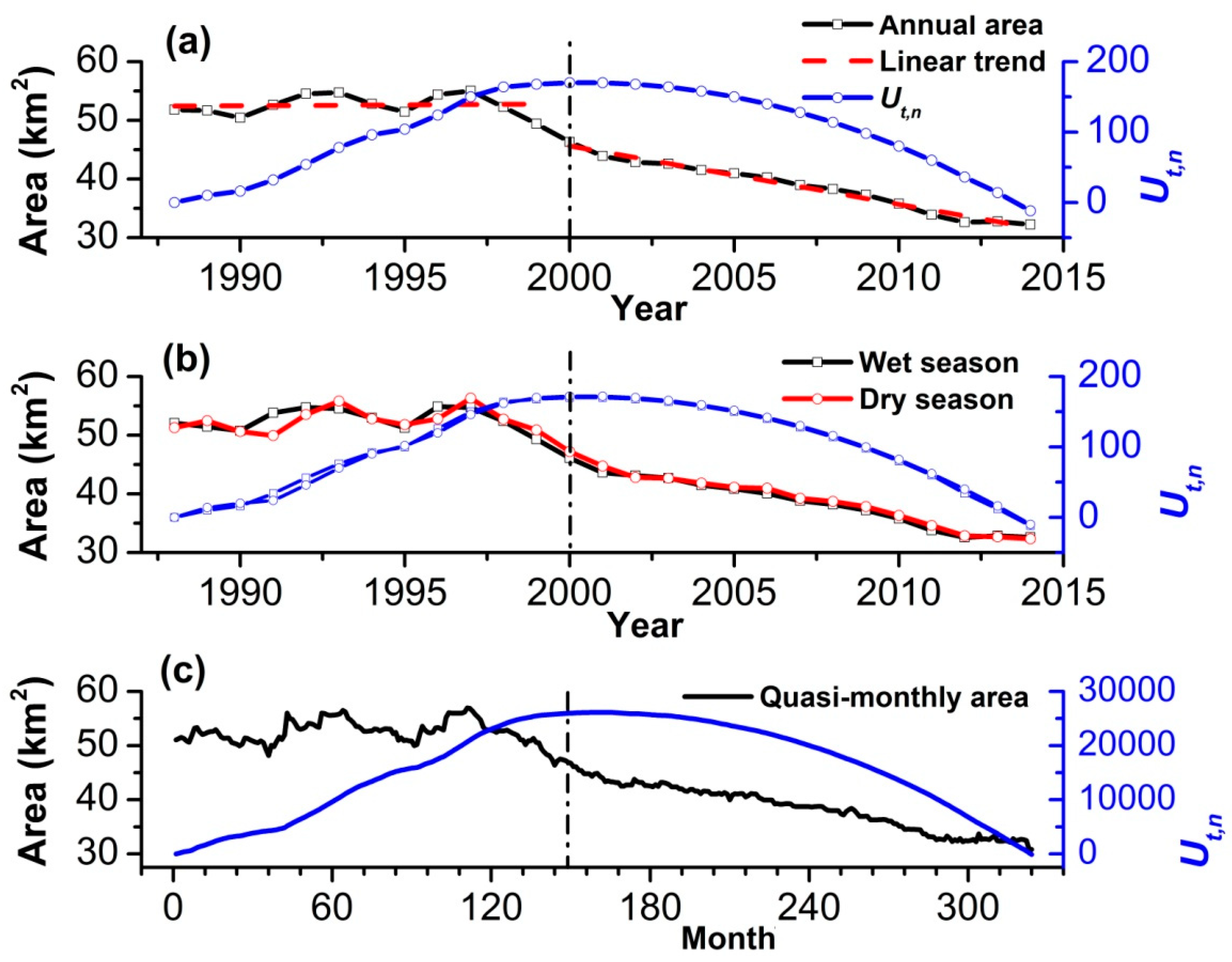
First, Figure 2a and Table 3 show the variations in the annual lake area and its basic statistics. During 1988−2014, the Hongjian Lake presented a large fluctuation. The mean value ($\overline{X}$), standard deviation (SD), and coefficient of variation (CV) of the annual lake area were 44.86 km², 7.86 km², and 0.18, respectively. The annual lake area had a significant declining trend (S) of −1.01 km²/year. When the Mann–Whitney statistic U_t,n in the Pettitt test was examined (blue solid line in Figure 2), the maximum $\left|U_{t,n}\right|$ was around the year 2000, and its calculated p-value was less than 0.05 (Equation (11)), which meant that there was one significant abrupt change point around the year 2000 examined by the Pettitt test. Therefore, the whole change process in the lake area could be divided into two distinct sub-phases, namely the slight ascending sub-phase with a small fluctuation in 1988–1999 and the significant monotonic declining sub-phase in 2000–2014. Specifically, in the first sub-period of 1988–1999, the $\overline{X}$, SD, CV, S, and Z of the annual lake area were 52.59 km², 1.79 km², 0.03, 0.07 km²/year, and 0.34 (not significant), respectively. In the second sub-period of 2000–2014, the average annual lake area ($\overline{X}$) dramatically decreased to 38.68 km², with a reduction ratio of 26.5% compared with that in 1988−1999. The volatility and change rate of the annual lake area during 2000–2014 increased, and the corresponding SD, CV, and S of the annual lake area changed to 4.48 km², 0.12, and −1.00 km²/year, respectively. The Z was equal to -5.05, which was significant at the 1% significance level.

Second, Figure 2b and Table 3 show the variations in the lake area in the wet season (May–October) and the dry season (November to April in the next year). During 1988–2014, whether in the wet or dry season, the overall change process and significant declining trend of the lake area were similar to that at the annual scale. The total significant downward trends were −0.99 km²/a in the wet season and −0.97 km²/a in the dry season. However, in the two sub-periods, there were still slight differences. In the first sub-period (1988–1999), the average lake area in the wet season (52.75 km²) was a little larger than that in the dry season (52.58 km²), but the ascending trend in the wet season (0.03 km²/a) was smaller than that in the dry season (0.10 km²/a). In the second sub-period (2000−2014), the $\overline{X}$, SD, CV, and significant S of the lake area in the wet season were 38.65 km², 4.42 km², 0.11, and −0.97 km²/year, respectively; the $\overline{X}$, SD, CV, and significant S in the dry season changed to 39.06 km², 4.58 km², 0.12, and −1.00 km²/year, respectively. The absolute values of all the basic statistics in the wet season were smaller than that in the dry season.

Third, Figure 2c and Table 3 show the variations in the lake area at a quasi-monthly scale. The lake area on the quasi-monthly scale had more subtle changes, which appeared to be more substantial, informative and winding on the variation process line. During 1988–2014, the $\overline{X}$, SD, CV, and significant trend (S) of the lake area on the quasi-monthly scale were 44.86 km², 7.78 km², 0.17, and −0.082 km²/month (i.e., −0.99 km²/year), respectively. In the first sub-period of 1988–1999, the lake area on the quasi-monthly scale belonged to a high-value and low-oscillation phase, namely with a high $\overline{X}$ (52.59 km²) and low CV (0.04); while the second sub-period of 2000−2014 became a low-value and high-oscillation phase, namely with a low $\overline{X}$ (38.68 km²) and high CV (0.11).

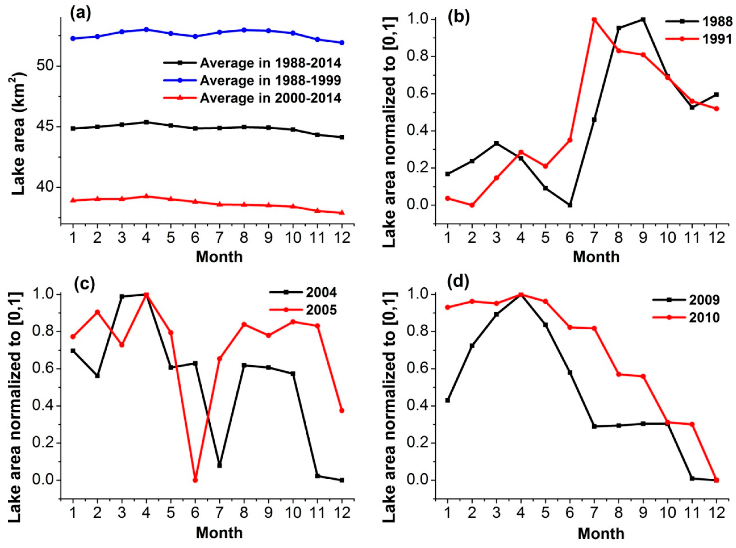
Lastly, the lake area at the intra-annual scale is shown in Figure 3 and

Table 4. Types of intra-annual variations in the Hongjian Lake area during 1988–2014.

Types a	Characteristics	Years
Type I	Bimodal: low peak on the left, high peak on the right	1988, 1991, 1992, 1994, 1995, 1996, 1998, 2002, 2003
Type II	Bimodal: high peak on the left, low peak on the right	1989, 1990, 2004, 2005, 2012, 2013, 2014
Type III	Unimodal: single peak on the left, declining on the right	1993, 1997, 1999, 2000, 2001, 2006, 2007, 2008, 2009, 2010, 2011

^a The representative diagrams of these three types are shown in Figure 3b–d.

. The intra-annual variations in the lake area during 1988−2014 had two peaks because there were two types of natural recharge in the lake basin, namely snowmelt runoff recharge in March−April and rainfall recharge in July−October. In the sub-period of 1988–1999, the intra-annual variations in the lake area also had two peaks, while in the second sub-period of 2000–2014, there was only one peak left in March–April (Figure 3a). When we took a closer look at the intra-annual changes each year, we found that the intra-annual variations in the lake area could be further divided into three types, namely type I, II, and III. Type I was a bimodal type, having one low peak on the left in March or April and one high peak on the right in July, August, or September. Type II was a bimodal type, with one high peak on the left in March or April and one low peak on the right in August, September, or October. Type III belonged to the unimodal type, with one single peak on the left in March or April and declining on the right. The years of type I were mainly concentrated before 2000, as well as the years of heavy precipitation in 2002 and 2003. The years of type II and III were concentrated after 2000, as well as some years of less precipitation (i.e., 1989, 1990, 1993, 1997, and 1999) (Table 4). For example, the intra-annual variations in the lake area in 1988 and 1991 belonged to type I, and the process of change exhibited a remarkable bimodal type: there was one low peak in March and one high peak in September in 1988, and there was one low peak in April and one high peak in July in 1991 (Figure 3b). The intra-annual variations in the lake area in 2004 and 2005 belonged to type II: there was one high peak in March or April and one low peak in August–October (Figure 3c). The intra-annual variations in the lake area in 1988 and 1991 belonged to type III: there was one peak in April, and then there was a stepped downward trend with no obvious peak after April (Figure 3d).

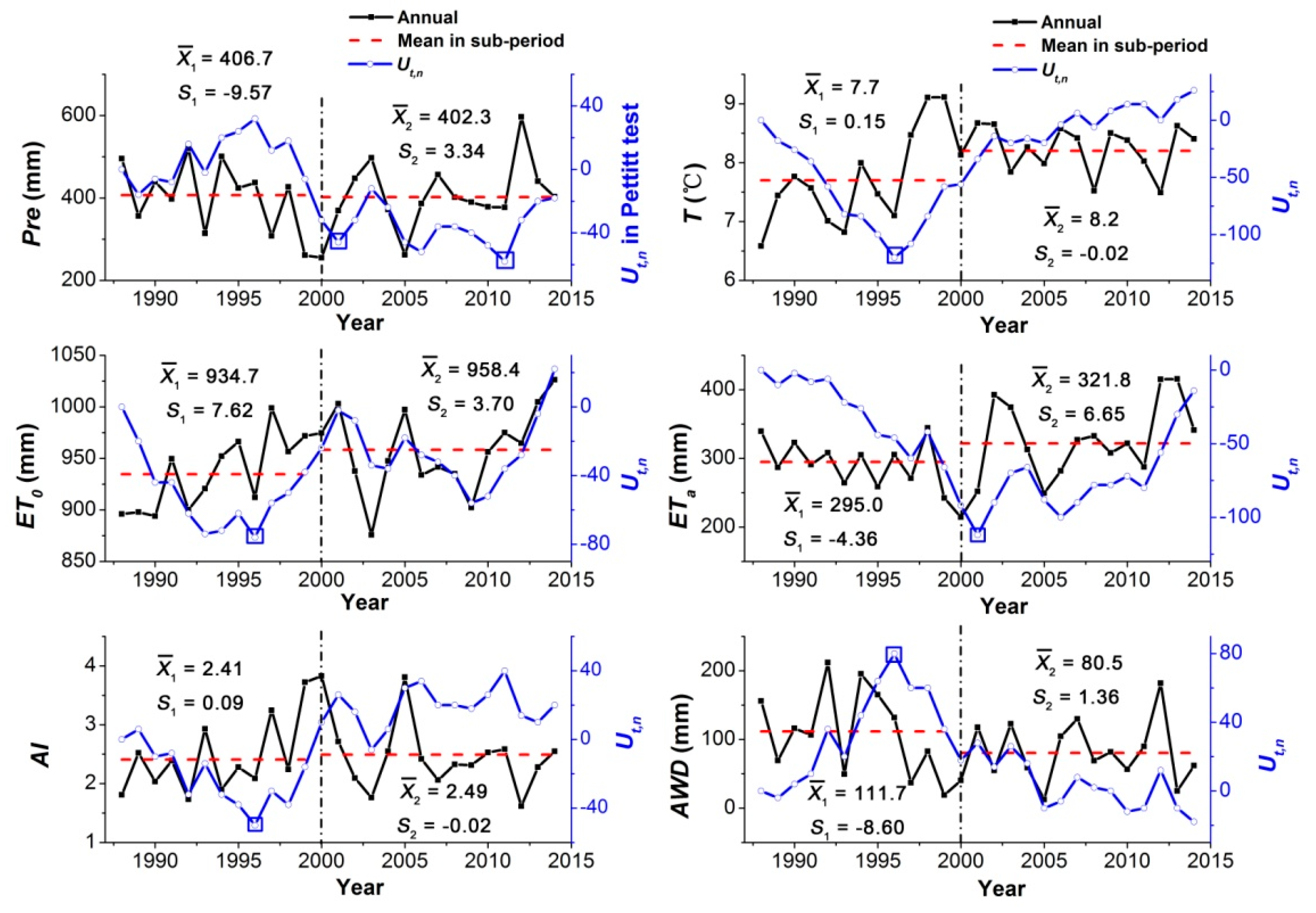
3.2. Variations in Climatic Factors at Multiple Time Scales

Similarly, we sequentially analyzed the corresponding variation characteristics of the six climatic factors closely related to lake area changes at annual, seasonal, monthly, and intra-annual scales. The turning points of these factors’ variation were different from that of the lake area. The turning point of precipitation (Pre) and actual evaporation (ET_a) was in the year 2001, and the turning point of temperature (T), potential evaporation (ET₀), aridity index (AI) and actual water difference (AWD) was in the year 1996 (Figure 4). However, to be consistent with the analysis of changes in the lake area, we had to use the same sub-periods of the lake area change as the dividing line of the climatic factor change.

The variations in the climatic factors at an annual scale are shown in Figure 4. During 1988–2014, the mean values of Pre, T, ET₀, ET_a, AI, and AWD were 404.3 mm, 8.0 °C, 947.8 mm, 309.9 mm, 2.46, and 94.4 mm, respectively. The overall fluctuation range of the factors was 4%–58%, in which the fluctuation range of T and ET₀ was less than 10%, and other factors (Pre, ET_a, AI, and AWD) were larger than 15%. Except for Pre and AWD with a declining trend of −0.38 mm/year and −2.62 mm/year, other indices (T, ET₀, ET_a, and AI) had an upward trend of 0.04 ℃/year, 2.77 mm/year, 1.79 mm/year, and 0.01 per year, respectively. The Mann–Kendall test’s statistic Z values of Pre, T, ET₀, ET_a, AI, and AWD were −0.04, 2.17 (significant at α = 0.05), 2.67 (significant at α = 0.01), 1.46, 0.75, and −1.38, respectively. Only the change trends of T and ET₀ were significant. When the study period was split into two sub-periods, each factor had some differences. The Pre and AWD in the first sub-period (1988–1999) were larger than in the second sub-period (2000–2014). The other factors (T, ET₀, ET_a, and AI) in 1988–1999 were smaller than in 2000–2014. This situation reflected the warming and drying of the climate in the second sub-period compared to in the first sub-period.

The variations in the climatic factors at the seasonal scale are shown in Figure 5. Whether during the entire study period (1988−2014) or for the two sub-periods (1988−1999 and 2000−2014), all the climatic factors showed large differences between the wet season (May−October) and the dry season (November−next April). Except for the aridity index (AI), the mean values ($\overline{X}$) of the other factors (Pre, T, ET₀, ET_a, and AWD) in the wet season were larger than that in the dry season. Except for the T and ET₀ having a low variation coefficient (CV < 0.05) in the wet season, the other factors had a large fluctuation both in the wet season and the dry season. The variation coefficient (CV) of these factors in the wet season was smaller than that in the dry season. The trends of T and ET₀ were higher than other factors. For example, during 1988−2014, the mean values ($\overline{X}$) of the Pre, T, ET₀, ET_a, AI, and AWD were 348.3 mm, 17.4 °C, 688.8 mm, 254.3 mm, 3.43, and 94.0 mm in the wet season, while $\overline{X}$ of these factors was equal to 56.0 mm, −1.5 °C, 258.7 mm, 55.6 mm, 5.91, and 0.4 mm in the dry season. The ratios of $\overline{X}$ in the wet season to the dry season were 6.2, −11.6, 2.7, 4.6, 0.6, and 235.0. The variation coefficient (CV) of Pre, ET_a, AI, and AWD was 0.17−0.57 in the wet season, and 0.51−61.24 in the dry season, respectively.

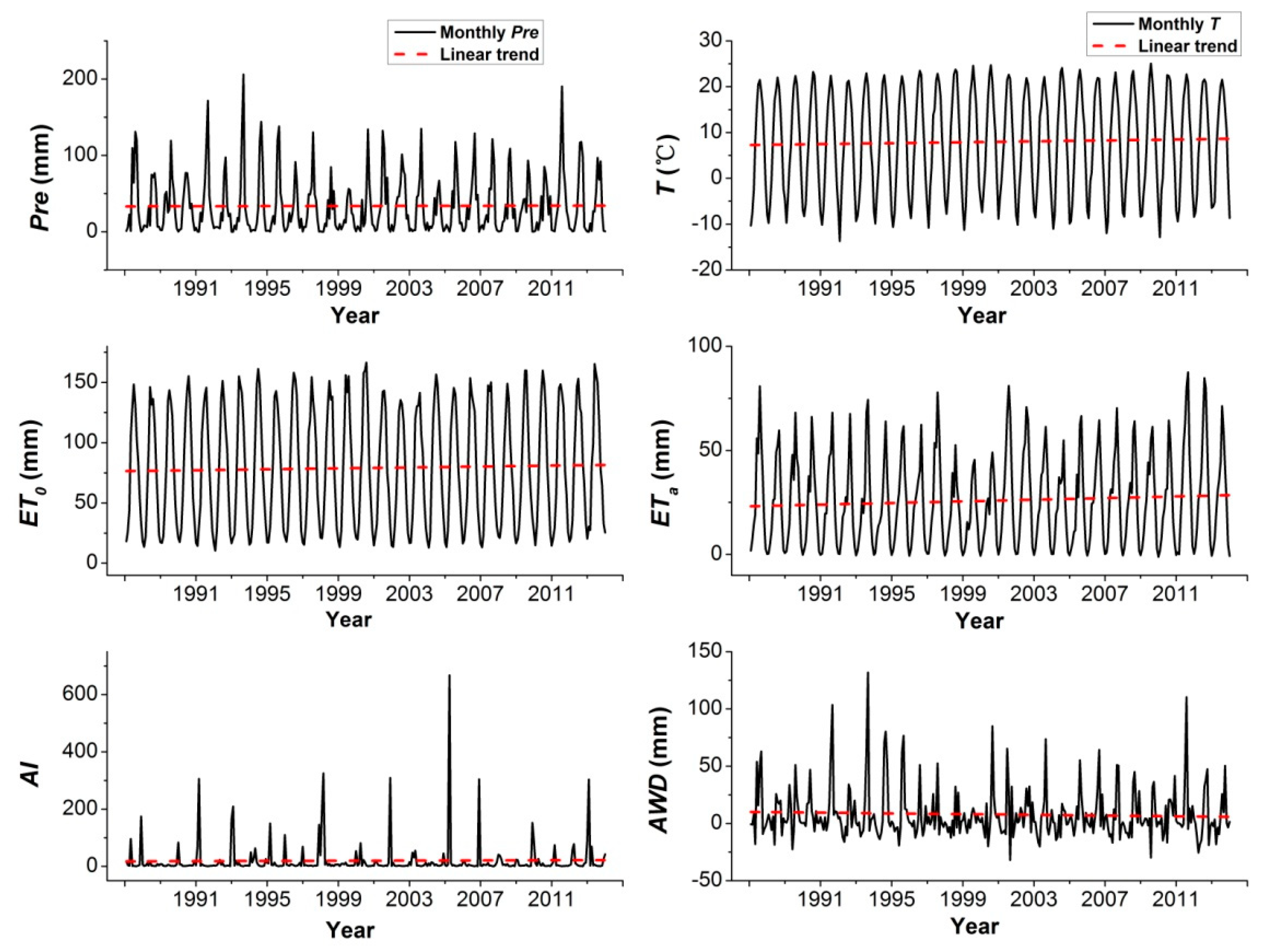
The variations in the climatic factors at a monthly scale are shown in Figure 6. During 1988−2014, each factor had a large fluctuation. The mean values ($\overline{X}$) of Pre, T, ET₀, ET_a, AI, and AWD at the monthly scale were 33.7 mm, 7.9 °C, 79 mm, 25.8 mm, 19.6, and 7.9 mm, respectively. The corresponding variation coefficient (CV) of Pre, T, ET₀, ET_a, AI, and AWD ranged from 0.62 to 3.02. Except for AWD having a negative change trend, the other factors had a positive change trend. The change trends of all the factors were not significant. When split into the two sub-periods, the mean values of six factors (Pre, T, ET₀, ET_a, AI, and AWD) in the first sub-period of 1988−1999 were 33.9 mm, 7.6 °C, 77.9 mm, 24.6 mm, 20.1, and 9.3 mm, respectively. In the second sub-period of 2000−2014, the mean value of six factors changed to 33.5 mm, 8.2 °C, 79.9 mm, 26.8 mm, 19.2, and 6.7 mm, respectively. The increase of T, ET₀, and ET_a, as well as the decrease of Pre and AWD, demonstrated that the climate in 2000−2014 generally became warmer and dryer.

The variations in the climatic factors at the intra-annual scale are shown in Figure 7. All the factors had obvious variations at the intra-annual scale, and all the factors in the two sub-periods had some differences. The Pre and AWD in 2000–2014 were smaller than that in 1988–1999, especially in March–May and July–August. Specifically, during 1988–1999, the average Pre was 17.7 mm in March, 22.5 mm in April, 36.0 mm in May, 103.6 mm in July, and 99.9 mm in August, respectively; differences of Pre between that in 2000–2014 and 1988–1999 were −6.2 mm in March, −1.4 mm in April, −1.2 mm in May, −16.3 mm in July, and −6.8 mm in August, respectively. The average AWD during 1988–1999 was 1.8 mm in March, −2.0 mm in April, 1.2 mm in May, 46.0 mm in July, and 42.4 mm in August, respectively; differences of AWD between that in 2000–2014 and 1988–1999 were −10.0 mm in March, −2.6 mm in April, −3.3 mm in May, −19.1 mm in July, and −12.7 mm in August, respectively. The T, ET₀, and ET_a in most months in 2000–2014 were larger than in 1988−1999. For example, differences of T in each month between that in 2000–2014 and 1988–1999 were 0.8 °C in January, 0.9 °C in February, 1.1 °C in March, 0.8 °C in April, 0.7 °C in May, 0.6 °C in June, 0.5 °C in July, 0.02 °C in August, 0.1 °C in September, 1.0 °C in October, 0.4 °C in November, and −0.6 °C in December, respectively.

3.3. Correlation between Lake Area and Climatic Factors

The correlation analysis results between the lake area and the six climatic factors at different scales (i.e., annual, wet season, dry season, and monthly) during 1988−2014 and the two sub-periods (1988−1999 and 2000−2014) are shown in

Table 5. Spearman correlation coefficient between the lake area and the six climatic factors at different scales during 1988−2014 and the two sub-periods (1988−1999 and 2000−2014).

Period	Scale	Pre	T	ET0	ETa	AI	AWD
1988−2014	Annual	−0.05a	−0.35	−0.32	−0.38	−0.06	0.19
	Wet season	−0.12	−0.36	−0.08	−0.36	0.23	0.01
	Dry season	0.06	−0.37	−0.47 *b	−0.36	−0.12	0.22
	Monthly	0.01	0.002	−0.0002	−0.03	−0.02	0.02
1988−1999	Annual	0.07	−0.29	0.14	0.06	−0.05	0.06
	Wet season	0.14	−0.26	0.04	0.02	−0.15	0.19
	Dry season	−0.20	−0.19	0.10	−0.03	0.15	−0.13
	Monthly	0.12	0.08	0.09	0.12	−0.11	0.003
2000−2014	Annual	−0.41	0.19	−0.29	−0.48	0.29	−0.12
	Wet season	−0.45	0.24	−0.12	−0.50	0.43	−0.22
	Dry season	0.13	−0.04	−0.28	−0.31	−0.15	0.30
	Monthly	−0.004	0.03	0.01	−0.04	−0.02	0.02

^a Italic numbers indicate the direction of the correlation is abnormal or contrary to the common direction. ^b * is significantly correlated at the 5% significance level (two-tailed), and the critical value and date set numbers at different scales are shown in Section 2.4.5.

. The Spearman correlation coefficients at different scales showed large differences. Regarding the magnitude of the correlation coefficient, the correlation coefficients at all scales were very low. The overall range of the correlation coefficients was from −0.50 to 0.43, and the absolute value of most correlation coefficients was less than 0.30. Even the absolute value of most correlation coefficients on the monthly scale was less than 0.10; no matter in which period or sub-period, the absolute values of the correlation coefficients at the annual scale and the wet season scale were generally higher than at the dry season scale and the monthly scale. Regarding the directionality of the correlation coefficient, regardless of in the entire study period or its two sub-periods, there was always a certain factor in the direction of the correlation coefficient that contradicts common sense (italic numbers labeled in Table 5), showing the opposite direction to common sense. For example, as the most important water resources for the lake, the precipitation (Pre) should be positively related to the lake, so the negative relationship is abnormal. This reversal of common sense was particularly evident in the second sub-period (2000−2014).

When further considering the lagged response, the lagged correlation analysis results between the lagged lake area and the six climatic factors at annual and monthly scales are shown in

Table 6. Spearman correlation coefficient for analysis to the lagged response of lake area and climatic factors on annual and monthly scales.

Period	Scale	Lag Time	Pre	T	ET0	ETa	AI	AWD
1988−2014	Annual	No	−0.05a	−0.35	−0.32	−0.38	−0.06	0.19
		1-yr	−0.02	−0.48 *b	−0.26	−0.33	−0.07	0.30
		2-yr	0.04	−0.45 *	−0.20	−0.28	−0.09	0.24
		3-yr	0.17	−0.56 **	−0.27	−0.16	−0.23	0.30
		4-yr	0.16	−0.61 **	−0.30	−0.13	−0.22	0.31
		5-yr	0.07	−0.65 **	−0.19	−0.12	−0.11	0.26
	Monthly	No	0.01	0.002	−0.0002	−0.03	−0.02	0.02
		1-m	0.01	−0.01	−0.01	−0.04	−0.02	0.03
		2-m	−0.01	−0.03	−0.03	−0.06	−0.01	0.04
		3-m	−0.03	−0.05	−0.04	−0.08	0.01	0.04
		6-m	−0.03	−0.06	−0.06	−0.08	0.001	0.03
		12-m	0.01	−0.01	0.02	−0.03	−0.001	0.04
1988−1999	Annual	No	0.07	−0.29	0.14	0.06	−0.05	0.06
		1-yr	0.09	−0.44	−0.10	−0.17	−0.12	0.32
		2-yr	0.44	0.20	−0.06	0.08	−0.41	0.52
		3-yr	0.10	0.36	−0.22	0.25	−0.12	−0.09
		4-yr	0.07	0.06	−0.55	0.33	−0.16	−0.14
		5-yr	−0.06	0.01	−0.08	−0.01	0.02	−0.09
	Monthly	No	0.12	0.08	0.09	0.12	−0.11	0.003
		1-m	0.15	0.07	0.09	0.14	−0.15	0.07
		2-m	0.13	0.03	0.06	0.10	−0.15	0.12
		3-m	0.07	−0.02	0.03	0.04	−0.08	0.09
		6-m	−0.04	−0.13	−0.11	−0.08	−0.03	0.01
		12-m	0.08	0.07	0.08	0.10	−0.04	0.04
2000−2014	Annual	No	−0.41	0.19	−0.29	−0.48	0.29	−0.12
		1-yr	−0.48	0.34	−0.06	−0.55 *	0.43	−0.23
		2-yr	−0.35	0.59 *	0.20	−0.29	0.31	−0.34
		3-yr	−0.31	0.47	0.40	−0.21	0.27	−0.33
		4-yr	−0.18	0.20	0.34	−0.29	0.13	−0.04
		5-yr	−0.11	−0.06	0.40	−0.30	0.07	0.10
	Monthly	No	−0.004	0.03	0.01	−0.04	−0.02	0.02
		1-m	−0.04	−0.003	−0.02	−0.08	0.01	0.01
		2-m	−0.08	−0.03	−0.06	−0.12	0.04	0.01
		3-m	−0.10	−0.06	−0.08	−0.15 *	0.06	−0.02
		6-m	−0.06	−0.01	−0.07	−0.11	0.02	0.02
		12-m	−0.04	0.05	0.04	−0.05	0.06	−0.04

^a Italic numbers indicate the direction of the correlation is abnormal or contrary to the common direction. ^b * and ** stand for significantly correlated at the 5% and 1% significance level (two-tailed test), and the critical value and date set numbers at different scales are shown in Section 2.4.5.

. In general, the lagged correlation coefficient was slightly increased compared to the normal (no-lagged) correlation coefficient, especially considering the lag period of nearly 3 years and nearly 3 months. Moreover, the directionality of some correlation coefficients that violate common sense had also changed. For example, the correlation coefficient between the lake area and Pre at the annual scale during 1988−2014 was −0.05, and the 3-year-lagged correlation coefficient was 0.17. It is worth noting that the lagged correlation coefficients at the monthly scale were still very low; in the second sub-period (2000−2014), the directionality of the correlation coefficient for most factors still appeared to be contrary to common sense.

When further considering the cumulative effect, the cumulative correlation analysis results between the cumulative lake area and the six cumulative climatic factors at multi scales are shown in

Table 7. Spearman correlation coefficients of cumulative anomaly sequence between lake area and climatic factors at different scales during 1988−2014 and the two sub-periods^a.

Period	Scale	Pre	T	ET0	ETa	AI	AWD
1988−2014	Annual	−0.22	−0.40 *	−0.13	−0.75 **	0.26	0.54 **
	Wet season	−0.19	−0.52 **	0.45 *	−0.69 **	0.60 **	0.48 *
	Dry season	0.11	−0.43 *	−0.84 **	−0.76 **	−0.004	0.43 *
	Monthly	−0.20 **	−0.25 **	−0.08	−0.68 **	0.04	0.55 **
1988−1999	Annual	0.30	−0.69 *	−0.52	−0.99 **	−0.45	0.80 **
	Wet season	0.34	−0.80 **	0.32	−0.98 **	0.40	0.72 **
	Dry season	0.06	−0.83 **	−0.96 **	−0.82 **	−0.08	0.21
	Monthly	0.43 **	−0.53 **	−0.31 **	−0.81 **	−0.19 *	0.85 **
2000−2014	Annual	−0.08	−0.94 **	0.02	−0.68 **	0.30	0.82 **
	Wet season	−0.14	−0.87 **	0.53 *	−0.61 *	0.81 **	0.72 **
	Dry season	0.32	−0.81 **	−0.90 **	−0.72 **	−0.25	0.77 **
	Monthly	0.04	−0.46 **	−0.05	−0.49 **	−0.05	0.80 **

^a * and ** stand for significantly correlated at the 5% and 1% significance level (two-tailed test), and the critical value and date set numbers at different scales are shown in Section 2.4.5. Italic numbers indicate the direction of the correlation is abnormal or contrary to the common direction.

. In general, the magnitude and significance of the cumulative correlation coefficient were increased compared to the normal (non-cumulative) correlation coefficient, especially for T, ET₀, ET_a, and AWD. For example, in the first sub-period of 1988−1999, the cumulative correlation coefficients for Pre, T, ET₀, ET_a, AI, and AWD at an annual scale were 0.30, −0.69 (significant), −0.52, −0.99 (significant), −0.45, and 0.80 (significant), respectively. Moreover, the cumulative correlation coefficients of all indicators on the monthly scale increased obviously. For example, during 1988−1999, the significant cumulative correlation coefficients for Pre, T, ET₀, ET_a, AI, and AWD at the monthly scale were 0.43, −0.53, −0.31, −0.81, −0.19, and 0.87, respectively. It is worth noting that the directionality of cumulative correlation coefficients for Pre and AI at all scales during 1988−2014 and on the annual, wet season, and monthly scale during 2000−2014 still appeared to be contrary to common sense.

When further jointly considering the lagged effect and the cumulative effect, the integrated lagged–cumulative correlation analysis results between the integrated lake area and the six cumulative climatic factors at annual and monthly scales are shown in

Table 8. Spearman correlation coefficients between lake area and climatic factors, while considering both lagged analysis (lag) and cumulative anomaly analysis (caa).

Period	Scale	Data Processing	Pre	T	ET0	ETa	AI	AWD
1988−2014	Annual	No	−0.05	−0.35	−0.32	−0.38	−0.06	0.19
		1-yr lag + caa	−0.002	−0.56 **	−0.23	−0.63 **	0.06	0.65 **
		2-yr lag+ caa	0.28	−0.61 **	−0.31	−0.65 **	−0.21	0.77 **
		3-yr lag+ caa	0.49 **	−0.69 **	−0.38	−0.64 **	−0.40 *	0.86 **
		4-yr lag + caa	0.55 **	−0.74 **	−0.47 *	−0.59 **	−0.51 **	0.91 **
		5-yr lag+ caa	0.62 **	−0.82 **	−0.63 **	−0.47 *	−0.63 **	0.91 **
	Monthly	No	0.01	0.002	−0.0002	−0.03	−0.02	0.02
		1-m lag + caa	−0.18 **	−0.27 **	−0.08	−0.67 **	0.02	0.57 **
		2-m lag + caa	−0.17 **	−0.28 **	−0.09	−0.65 **	0.03	0.57 **
		3-m lag + caa	−0.15 **	−0.28 **	−0.10	−0.65 **	0.02	0.56 **
		6-m lag+ caa	−0.09	−0.33 **	−0.13 *	−0.64 **	0.01	0.63 **
		12-m lag+ caa	0.01	−0.37 **	−0.13 *	−0.59 **	0.06	0.67 **
1988−1999	Annual	No	0.07	−0.29	0.14	0.06	−0.05	0.06
		1-yr lag + caa	0.80 **	−0.88 **	−0.71 **	−0.80 **	−0.87 **	0.91 **
		2-yr lag + caa	0.94 **	−0.98 **	−0.82 **	−0.70 *	−0.94 **	0.94 **
		3-yr lag + caa	0.83 **	−0.99 **	−0.89 **	−0.27	−0.91 **	0.82 **
		4-yr lag + caa	0.76 **	−0.98 **	−0.87 **	−0.53	−0.84 **	0.82 **
		5-yr lag + caa	0.73 **	−0.97 **	−0.91 **	−0.20	−0.83 **	0.81 **
	Monthly	No	0.12	0.08	0.09	0.12	−0.11	0.003
		1-m lag + caa	0.46 **	−0.55 **	−0.32 **	−0.81 **	−0.25 **	0.86 **
		2-m lag + caa	0.47 **	−0.58 **	−0.35 **	−0.80 **	−0.27 **	0.87 **
		3-m lag + caa	0.49 **	−0.60 **	−0.39 **	−0.79 **	−0.31 **	0.87 **
		6-m lag + caa	0.59 **	−0.68 **	−0.55 **	−0.76 **	−0.42 **	0.89 **
		12-m lag + caa	0.69 **	−0.67 **	−0.46 **	−0.68 **	−0.44 **	0.91 **
2000−2014	Annual	No	−0.41	0.19	−0.29	−0.48	0.29	−0.12
		1-yr lag + caa	0.15	−0.96 **	0.004	−0.48	0.18	0.82 **
		2-yr lag+ caa	0.25	−0.98 **	−0.26	−0.46	−0.06	0.84 **
		3-yr lag+ caa	0.35	−0.99 **	−0.43	−0.73 **	−0.34	0.94 **
		4-yr lag + caa	0.53 *	−0.99 **	−0.59 *	−0.50	−0.51	0.94 **
		5-yr lag+ caa	0.59 *	−0.99 **	−0.70 **	−0.47	−0.65 **	0.95 **
	Monthly	No	−0.004	0.03	0.01	−0.04	−0.02	0.02
		1-m lag + caa	0.07	−0.45 **	−0.04	−0.47 **	0.03	0.79 **
		2-m lag + caa	0.11	−0.44 **	−0.03	−0.45 **	0.02	0.81 **
		3-m lag + caa	0.14	−0.44 **	−0.01	−0.45 **	0.04	0.82 **
		6-m lag + caa	0.14	−0.40 **	0.19 **	−0.44 **	0.10	0.80 **
		12-m lag + caa	0.29 **	−0.49 **	0.12	−0.34 **	−0.12	0.83 **

^a Italic numbers indicate the direction of the correlation is abnormal or contrary to the common direction. * and ** stand for significantly correlated at the 5% and 1% significance level (two-tailed test), and the critical value and date set numbers at different scales are shown in Section 2.4.5.

. The lagged–cumulative correlation coefficient at annual and monthly scales further improved in size, directionality, and significance. Taking the first sub-period with the most significant improvement effect as an example, during 1988−1999, the significant 2-year-lagged–cumulative correlation coefficients for Pre, T, ET₀, ET_a, AI, and AWD at the annual scale were 0.94, −0.98, −0.82, −0.70, −0.94, and 0.94, respectively. The significant 3-month-lagged–cumulative correlation coefficients for Pre, T, ET₀, ET_a, AI, and AWD at a monthly scale were 0.49, −0.60, −0.39, −0.79, −0.31, and 0.87, respectively. It is still worth noting that the directionality of lagged–cumulative correlation coefficients for Pre and AI at a monthly scale during 1988−2014 and on a monthly scale during 2000−2014 still slightly appeared to be contrary to common sense.

Overall, according to the corresponding results from the Table 5, Table 6, Table 7 and Table 8, when we gradually considered the four cases or scenarios of progressive Spearman correlation analysis schemes (see in Table 2), namely case 1 (original correlation analysis), case 2 (lagged correlation analysis), case 3 (cumulative correlation analysis), and case 4 (lagged and cumulative correlation analysis), the lagged effect and cumulative effect were gradually reflected and displayed by the increase of the correlation coefficient, the reasonable change in the direction of the correlation coefficient, and the significant improvement of the correlation coefficient.

4. Discussion

4.1. Lake Shrinkage in This Study and Other Endorheic Basins

Due to the influence of current climate warming and intensified human activities, whether in the Ordos endorheic (inflow) region where our study area is located or the larger inland area in northwest China and other famous inland regions worldwide, severe lake shrinkage has been encountered in recent decades. For example, in the Ordos endorheic region, Yan et al. [47] studied the changes of the Bojiang Lake area using the Landsat remote sensing data and revealed that the average lake area significantly declined from 8.86 km² in 1980–1998 to 3.50 km² in 1999–2013, with average change rates of -60.5% and a changing trend of −0.75 km²/year in 1999−2013. Liang and Yan [34] studied the changes in the annual Hongjian Lake area in the Ordos endorheic region using Landsat images and revealed that the average change rates and trends during 1999–2015, compared with those in 1988–1998, were -26.5% and -1.04 km²/year, respectively. In northwest China, Bai et al. [13] applied Landsat imageries to find that Bosten Lake, as the largest inland freshwater lake in China, declined from 1,055.83 km² in 1975 to 958.90 km² in 2007, with an average change rate of −9.18% and a changing trend of −2.94 km²/year. Guo et al. [19] also revealed that the area of Bosten Lake decreased by −348 km² from 2003 to 2010, with an average declining trend of −43.50 km²/year. In Central Asia, Bai et al. [13] used Landsat imageries to reveal the lake area of the Aral Sea, once the world’s fourth-largest lake, which decreased from 59,262.35 km² in 1975 to 14,400.15 km² in 2007, with a change rate of −75.70% and average change trend of −1359.46 km²/year. Chaudhari et al. [15] used Landsat imageries to reveal that Urmia Lake in northwestern Iran, the largest lake in the Middle East and once the second-largest saline lake worldwide, decreased from approximately 5000 km² in 1987 to 1150 km² in 2016, with a shrinkage rate of −77% and average declining trend of −128.33 km²/year. In our study, Hongjian Lake declined on average by 52.99 km² annually in 1988–1999 to 38.68 km² in 2000–2014, with a declining ratio of -26.5%, and by −1.00 km²/year in 2000–2014. Therefore, the shrinkage rate and trend in our study were within the scope of these cited research results.

Comparing these studies, we find that lake wetland shrinkage is a relatively common phenomenon, especially in endorheic basins which spatially concur with arid and semi-arid climate regions. These endorheic lakes have suffered severe shrinkage, but there are still significant differences in the size and rate of change in the lake area due to differences in remote sensing data sources, data time ranges, trend estimation method, regional climatic conditions, and the anthropogenic disturbance intensity. These differences reflect the complexity and regional differences of inland lake changes. These regional differences and their hidden mechanisms are worthy of in-depth comparative research in the future. The issues regarding the lagged response and cumulative effect initially revealed in this study are worthy of further exploration. A comprehensive comparison of the lagged response characteristics and cumulative effects between different endorheic basins or regions worldwide will be very interesting.

Whether in the research cited in this study or in other related research that is not cited in this study, the nonparametric statistical approach is the preferred methodology for studies on the variations of the lake itself, climatic and anthropogenic factors, and the relationships between the lake and the factors. Nonparametric statistical methods have the advantages that they require few assumptions about the underlying populations, are often easier to apply than the normal theory counterparts, enable the user to obtain exact p-values for tests, have robustness for non-normally distributed data, and are insensitive to outlier and missing data [78]. The combined use of non-parametric methods has a certain reference significance for similar research and is highly recommended, such as the Sen’s slope estimator method [63], the Mann–Kendall test [66,67], the Pettitt test [72], and the Spearman rank correlation test [75] used in this study. In addition, the design ideas and design schemes of the correlation analysis in this study (Section 2.4.5 and Table 2) play a key role in investigating the lagged response effect and cumulative effect, which has a certain reference significance for other related research on lake wetlands.

4.2. Implications for Lake Wetland Protection in Endorheic Basins

First, we reveal that both for the continuous linear decline of the annual lake area or the morphological change in the curve of intra-annual variation process, it is fully explained that the natural rhythm of the lake change has been broken, and the actual changes of lake area are not well explained by climatic forcing, which indicates that the lake area change is impacted more by the intensive human activities. The annual lake area has been decreasing year by year since 1999 or 2000, and this decline has almost continued to decline linearly, which is totally incompatible with the natural rhythm of climatic dry–wet conditions. Before 2000, the curve of the annual variation of the lake area clearly showed a “double peak” pattern or bimodal type, which is basically consistent with the natural intra-annual rhythm of climate change; however, this natural “double peak” pattern was obviously artificially broken after 2000. The “double peak” form has evolved into a “single peak” form or unimodal type, and even shows a linear decline pattern that decreases month by month. This pattern change will only recover to a certain degree when the precipitation is much larger than the average. For example, in 2002, 2003, 2012, and 2013, the precipitation in these years was 36–192 mm larger than the mean value. Liang et al. [34] showed sharp increasing variations in the annual human activities during 1988–2015, using the seven representative indicators (i.e., area of land use types, Normalized Differential Vegetation Index, human population, sheep population, gross industrial output value, hydraulic engineering construction, and tourism development), and revealed that the human activities had a more important influence on the lake area change after 1999. These studies have jointly demonstrated that, since the late 1990s or early 21st century, human activities have become the dominant factor in the change of the lake area. However, due to the lack of data on human activities on a monthly scale, we are unable to determine the response characteristics of the lake area to human activities. It is urgent to collect more detailed human activity data from multiple sources, and we recommend that the monitoring of water use data for human activities must be strengthened to provide available data support for subsequent research. Under the influence of such strong human activities, reasonably controlling human activities to reduce human water use in the basin has become a new core task of water resource management.

Second, to make matters worse, climate change has also cast a shadow over the protection of the endorheic lake wetland. Our results showed that, during 1988−2014, whether on the annual scale, dry and wet season scale, or monthly scale, the average climate of the basin was generally warming and drying, mainly reflected by the increase in temperature (T), arid index (AI) and evaporation (ET₀, ET_a), and the decrease in the precipitation (Pre) and actual water difference (AWD) (Figure 4). When we checked this change on the intra-annual scale (2000−2014 vs. 1988−1999), we further found that Pre and AWD mainly reduced in March−May and July−August, which coincides with the peak of the snowmelt recharge in March and rainfall recharge in July−August of the lake, while T and ET_a increased in most months except December. This climatic warming and drying have led to water deficits in the lake basin, and the lake area has accordingly shrunk on the annual scale, dry and wet season scale, and monthly scale since the late 1990s or early 21st century. We also found that lake changes have a lagging response to climate change, with a lag period of about 1−3 years on the annual scale and 1−3 months on a monthly scale. This means that the size of the lake area in a certain year is significantly affected by the climatic dry−wet regime of the previous three years, and the size of the lake area in a certain month is obviously affected by the climatic dry−wet conditions for the past three months. Hence, for a natural closed endorheic lake basin like the Hongjian Lake, without the supply of other external water sources, the change in the lake area is largely controlled by changes in the climatic conditions within the basin itself—especially the climatic dry−wet regime in recent months and in recent years. This high susceptibility to climate change is an inherent property of closed basins, and relevant authorities must clearly recognize the fundamental water scarcity and the natural vulnerability of water resources.

5. Conclusions

In this study, using Landsat remote sensing images and the Modified Normalized Difference Water Index, we obtained the Hongjian Lake area changes on annual, seasonal, and quasi-monthly scales during 1988−2014, analyzed the corresponding variations of six climatic factors using satellite-based products, and investigated the relationships between changes in the lake area and changes in these climatic factors. Some conclusions can be drawn as follows. (1) There was a small numerical difference in the size and change trend of the lake area between multiple scales, and the quasi-monthly lake area had a more subtle, dense and tortuous variation process line. However, whether on the annual scale, seasonal scale or monthly scale, the change of lake area showed a similar significant decline during 1988−2014, and this process can be divided into two sub-stages, namely the first sub-phase with a large area and a slight increase in 1988−1999, and the second sub-phase with a small area and a significant decrease in 2000−2014. (2) The intra-annual lake area change process showed three types, and it presented the natural bimodal type I in most years in the sub-period of 1988−1999, featuring one low snowmelt runoff recharge peak in March−April and one high rainfall recharge peak in July−September, which is compatible with the natural rhythm of climatic dry−wet conditions; however, as the natural rhythm of the lake changes has been broken by intensive human activities since the late 1990s or early 21st century, the natural bimodal type I has obviously changed into non-natural bimodal type II and unimodal type III, featured by a declining peak in July−September. (3) The climatic dry−wet regime on multi-scales during 1988−2014 in the endorheic Hongjian Lake Basin was generally warming and drying, which is mainly reflected by the increase in temperature (T), arid index (AI) and evaporation (ET₀, ET_a), and the decrease in the precipitation (Pre) and actual water difference (AWD). There were large differences in the climatic factors at different time scales, especially in the wet and dry seasons. The fluctuation size of climate change at different scales was ranked, in descending order, as the monthly scale, dry season scale, wet season scale, and annual scale. (4) When the lagged effect and cumulative effect were not considered, the correlation coefficient between the lake area and climatic factors was very low, with most values lower than 0.30, and the direction of correlation was not correct; whereas, when gradually considering the lagged effect, the cumulative effect, and the lagged and cumulative combined effect, most correlation coefficients significantly increased to 0.50−0.99, and the direction of the correlation coefficient became coincident with common sense. The correlation analysis identified a lag period of approximately 1−3 years on an annual scale and a lag period of approximately 1−3 months on a monthly scale. This high vulnerability to climate change will mean that lake water management and watershed ecological protection bodies will continue to face high pressures and arduous challenges.

References

1. Nichols, G. Endorheic Basins. In Tectonics of Sedimentary Basins: Recent Advances; John Wiley & Sons: Hoboken, NJ, USA, 2011; pp. 621–632. [Google Scholar]
2. Sawe, B.E. Fluvial landforms: What Is an Endorheic Basin? WorldAtlas. Available online: https://www.worldatlas.com/articles/fluvial-landforms-what-is-an-endorheic-basin.html (accessed on 1 September 2019).
3. Wang, J.; Song, C.; Reager, J.T.; Yao, F.; Famiglietti, J.S.; Sheng, Y.; MacDonald, G.M.; Brun, F.; Schmied, H.M.; Marston, R.A.; et al. Recent global decline in endorheic basin water storages. Nat. Geosci. 2018, 11, 926–932. [Google Scholar] [CrossRef] [PubMed] [Green Version]
4. Yapiyev, V.; Sagintayev, Z.; Inglezakis, V.; Samarkhanov, K.; Verhoef, A. Essentials of endorheic basins and lakes: A review in the context of current and future water resource management and mitigation activities in central asia. Water 2017, 9, 798. [Google Scholar] [CrossRef] [Green Version]
5. Birkett, C.M.; Mason, I.M. A new global lakes database for a remote sensing program studying climatically sensitive large lakes. J. Great Lakes Res. 1995, 21, 307–318. [Google Scholar] [CrossRef]
6. Palmer, S.C.J.; Kutser, T.; Hunter, P.D. Remote sensing of inland waters: Challenges, progress and future directions. Remote Sens. Environ. 2015, 157, 1–8. [Google Scholar] [CrossRef] [Green Version]
7. Williamson, C.E.; Saros, J.E.; Vincent, W.F.; Smol, J.P. Lakes and reservoirs as sentinels, integrators, and regulators of climate change. Limnol. Oceanogr. 2009, 54, 2273–2282. [Google Scholar] [CrossRef]
8. Mao, D.; Wang, Z.; Wu, J.; Wu, B.; Zeng, Y.; Song, K.; Yi, K.; Luo, L. China’s wetlands loss to urban expansion. Land Degrad. Dev. 2018, 29, 2644–2657. [Google Scholar] [CrossRef]
9. Wurtsbaugh, W.A.; Miller, C.; Null, S.E.; DeRose, R.J.; Wilcock, P.; Hahnenberger, M.; Howe, F.; Moore, J. Decline of the world’s saline lakes. Nat. Geosci. 2017, 10, 816. [Google Scholar] [CrossRef]
10. Li, X.; Cheng, G.; Ge, Y.; Li, H.; Han, F.; Hu, X.; Tian, W.; Tian, Y.; Pan, X.; Nian, Y. Hydrological cycle in the heihe river basin and its implication for water resource management in endorheic basins. J. Geophys. Res. Atmos. 2018, 123, 890–914. [Google Scholar] [CrossRef]
11. Chen, J.L.; Pekker, T.; Wilson, C.R.; Tapley, B.D.; Kostianoy, A.G.; Cretaux, J.F.; Safarov, E.S. Long-term caspian sea level change. Geophys. Res. Lett. 2017, 44, 6993–7001. [Google Scholar] [CrossRef]
12. Micklin, P. The past, present, and future aral sea. Lakes Reserv. Res. Manag. 2010, 15, 193–213. [Google Scholar] [CrossRef]
13. Bai, J.; Chen, X.; Li, J.; Yang, L.; Fang, H. Changes in the area of inland lakes in arid regions of central asia during the past 30 years. Environ. Monit. Assess. 2011, 178, 247–256. [Google Scholar] [CrossRef] [PubMed]
14. Stone, R. Saving iran’s great salt lake. Science 2015, 349, 1044–1047. [Google Scholar] [CrossRef] [PubMed]
15. Chaudhari, S.; Felfelani, F.; Shin, S.; Pokhrel, Y. Climate and anthropogenic contributions to the desiccation of the second largest saline lake in the twentieth century. J. Hydrol. 2018, 560, 342–353. [Google Scholar] [CrossRef]
16. Okpara, U.T.; Stringer, L.C.; Dougill, A.J. Lake drying and livelihood dynamics in lake chad: Unravelling the mechanisms, contexts and responses. Ambio 2016, 45, 781–795. [Google Scholar] [CrossRef] [Green Version]
17. Gao, H.; Bohn, T.J.; Podest, E.; McDonald, K.C.; Lettenmaier, D.P. On the causes of the shrinking of lake chad. Environ. Res. Lett. 2011, 6, 034021. [Google Scholar] [CrossRef] [Green Version]
18. Fan, Z.; Alishir, K.; Xu, H.; Zhang, Q. Changes of tarim river and evolution of lop nur. Quat. Sci. 2009, 29, 232–240. (In Chinese) [Google Scholar]
19. Guo, M.; Wu, W.; Zhou, X.; Chen, Y.; Li, J. Investigation of the dramatic changes in lake level of the bosten lake in northwestern china. Theor. Appl. Climatol. 2015, 119, 341–351. [Google Scholar] [CrossRef]
20. Gao, H. Satellite remote sensing of large lakes and reservoirs: From elevation and area to storage. Wires Water 2015, 2, 147–157. [Google Scholar] [CrossRef]
21. Alsdorf, D.E.; Rodríguez, E.; Lettenmaier, D.P. Measuring surface water from space. Rev. Geophys. 2007, 45. [Google Scholar] [CrossRef]
22. Berry, P.A.M.; Garwick, J.D.; Freeman, J.A.; Mathers, E.L. Global inland water monitoring from multi-mission altimetry. Geophys. Res. Lett. 2005, 32, 101–120. [Google Scholar] [CrossRef]
23. Lehner, B.; Döll, P. Development and validation of a global database of lakes, reservoirs and wetlands. J. Hydrol. 2004, 296, 1–22. [Google Scholar] [CrossRef]
24. Verpoorter, C.; Kutser, T.; Seekell, D.A.; Tranvik, L.J. A global inventory of lakes based on high-resolution satellite imagery. Geophys. Res. Lett. 2014, 41, 6396–6402. [Google Scholar] [CrossRef]
25. Singh, A.; Seitz, F.; Schwatke, C. Inter-annual water storage changes in the aral sea from multi-mission satellite altimetry, optical remote sensing, and grace satellite gravimetry. Remote Sens. Environ. 2012, 123, 187–195. [Google Scholar] [CrossRef]
26. Schneider, S.R.; McGinnis, D.F.; Stephens, G. Monitoring africa’s lake chad basin with landsat and noaa satellite data. Int. J. Remote Sens. 1985, 6, 59–73. [Google Scholar] [CrossRef]
27. Pu, P.; Tu, Q.; Wang, S. Research progress of limnology in China. J. Lake Sci. 1989, 6, 1–11. (In Chinese) [Google Scholar]
28. Zhang, G.; Yao, T.; Shum, C.K.; Yi, S.; Yang, K.; Xie, H.; Feng, W.; Bolch, T.; Wang, L.; Behrangi, A.; et al. Lake volume and groundwater storage variations in tibetan plateau’s endorheic basin. Geophys. Res. Lett. 2017, 44, 5550–5560. [Google Scholar] [CrossRef]
29. Shen, F.; Kuang, D. Remote sensing investigation and survey of qinghai lake in the past 25 years. J. Lake Sci. 2003, 15, 289–296. (In Chinese) [Google Scholar]
30. Ma, M.; Wang, X.; Veroustraete, F.; Dong, L. Change in area of ebinur lake during the 1998–2005 period. Int. J. Remote Sens. 2007, 28, 5523–5533. [Google Scholar] [CrossRef]
31. Tang, K.; Wang, H.; Liu, C. Preliminary study of hongjiannao lake’s variation and ecological water demand. J. Nat. Resour. 2003, 18, 304–309. (In Chinese) [Google Scholar]
32. BirdLifeInternational. Larus relictus. The Iucn Red List of Threatened Species 2016; BirdLifeInternational: Cambridge, UK, 2019. [Google Scholar] [CrossRef]
33. Xiao, H.; Zhang, Z.; Wang, Z.; Wang, Y. Breding population dynamic of relict gull (laurs relietus) at hongjiannao lake of shaanxi province. J. Shaanxi Norm. Univ. Nat. Sci. Ed. 2006, 34, 83–86. (In Chinese) [Google Scholar]
34. Liang, K.; Yan, G. Application of landsat imagery to investigate lake area variations and relict gull habitat in hongjian lake, ordos plateau, China. Remote Sens. 2017, 9, 1019. [Google Scholar] [CrossRef] [Green Version]
35. Zhao, N.; Ma, C.; Yang, Y. Water quality variation of lake hongjiannao and its driving force analysis from 1973 to 2013. J. Lake Sci. 2016, 28, 982–993. (In Chinese) [Google Scholar]
36. Liu, P.; Gan, W.; Zhang, R.; Tan, L. Quantitative analysis on water volume change and impacting factors for hongjiannao watershed in northern shaanxi province. J. Xi’an Jiaotong Univ. 2009, 43, 119–124. (In Chinese) [Google Scholar]
37. Yang, L.; Huang, Q.; Wu, J.; Jia, Z. Influence factors and prediction on area change of lake hongjiannao. J. Arid Land Resour. Environ. 2014, 28, 74–78. (In Chinese) [Google Scholar]
38. Ma, B.; Wu, L.; Zhang, X.; Li, X.; Liu, Y.; Wang, S. Locally adaptive unmixing method for lake-water area extraction based on modis 250m bands. Int. J. Appl. Earth Obs. Geoinf. 2014, 33, 109–118. [Google Scholar] [CrossRef]
39. Yin, L.; Zhang, M.; Dong, J. Area variation and controlling factors of lake hongjian, mu us desert, china based on remote sensing techniques. Geol. Bull. China 2008, 27, 1151–1156. (In Chinese) [Google Scholar]
40. Wang, J.; Qu, J.; Zhang, W. Extraction and monitoring of hongjiannao lake area in mu us sandy land based on mixed pixel decomposition of remote sensing data. J. Desert Res. 2011, 31, 558–562. (In Chinese) [Google Scholar]
41. Liu, Y.; Wu, L.; Yue, H. Monitoring of hongjiannao lake area based on landsat and hj imageries. Geogr. Geo-Inf. Sci. 2015, 31, 60–64. (In Chinese) [Google Scholar]
42. Liang, K. Spatio-temporal variations in precipitation extremes in the endorheic hongjian lake basin in the ordos plateau, china. Water 2019, 11, 1981. [Google Scholar] [CrossRef] [Green Version]
43. Zhang, H.; Liu, P.; Li, X. Land use dynamic change of hongjiannao watershed in northern shaanxi province. Environ. Sci. Technol. 2011, 34, 180–183. (In Chinese) [Google Scholar]
44. UNEP-WCMC. Species+ Larus Relictus. Available online: https://www.speciesplus.net/#/taxon_concepts/9314/legal (accessed on 1 September 2019).
45. Zheng, G.; Wang, Q. China Red Data Book of Endangered Animals (AVES); Science Press: Beijing, China, 1998. [Google Scholar]
46. Xu, H. Modification of normalised difference water index (ndwi) to enhance open water features in remotely sensed imagery. Int. J. Remote Sens. 2006, 27, 3025–3033. [Google Scholar] [CrossRef]
47. Yan, G.; Lou, H.; Liang, K.; Zhang, Z. Dynamics and driving forces of bojiang lake area in erdos larus relictus national nature reserve, china. Quat. Int. 2018, 475, 16–27. [Google Scholar] [CrossRef]
48. Liang, K. Quantifying streamflow variations in ungauged lake basins by integrating remote sensing and water balance modelling: A case study of the erdos larus relictus national nature reserve, China. Remote Sens. 2017, 9, 588. [Google Scholar] [CrossRef] [Green Version]
49. Yang, X.; Qin, Q.; Grussenmeyer, P.; Koehl, M. Urban surface water body detection with suppressed built-up noise based on water indices from sentinel-2 msi imagery. Remote Sens. Environ. 2018, 219, 259–270. [Google Scholar] [CrossRef]
50. McFeeters, S.K. The use of the normalized difference water index (ndwi) in the delineation of open water features. Int. J. Remote Sens. 1996, 17, 1425–1432. [Google Scholar] [CrossRef]
51. Stocker, T. Climate Change 2013: The Physical Science Basis: Working Group I Contribution to the Fifth Assessment Report of the Intergovernmental Panel on Climate Change; Cambridge University Press: Cambridge, UK, 2014. [Google Scholar]
52. Beck, H.E.; Van Dijk, A.I.; Levizzani, V.; Schellekens, J.; Gonzalez Miralles, D.; Martens, B.; De Roo, A. Mswep: 3-hourly 0.25 global gridded precipitation (1979–2015) by merging gauge, satellite, and reanalysis data. Hydrol. Earth Syst. Sci. 2017, 21, 589–615. [Google Scholar] [CrossRef] [Green Version]
53. Bai, P.; Liu, X. Evaluation of five satellite-based precipitation products in two gauge-scarce basins on the tibetan plateau. Remote Sens. 2018, 10, 1316. [Google Scholar] [CrossRef] [Green Version]
54. Liu, J.; Shangguan, D.; Liu, S.; Ding, Y.; Wang, S.; Wang, X. Evaluation and comparison of chirps and mswep daily-precipitation products in the qinghai-tibet plateau during the period of 1981–2015. Atmos. Res. 2019, 230, 104634. [Google Scholar] [CrossRef]
55. Miralles, D.G.; Holmes, T.R.H.; De Jeu, R.A.M.; Gash, J.H.; Meesters, A.G.C.A.; Dolman, A.J. Global land-surface evaporation estimated from satellite-based observations. Hydrol. Earth Syst. Sci. 2011, 15, 453–469. [Google Scholar] [CrossRef] [Green Version]
56. Martens, B.; Miralles, D.G.; Lievens, H.; van der Schalie, R.; de Jeu, R.A.M.; Fernández-Prieto, D.; Beck, H.E.; Dorigo, W.A.; Verhoest, N.E.C. Gleam v3: Satellite-based land evaporation and root-zone soil moisture. Geosci. Model Dev. 2017, 10, 1903–1925. [Google Scholar] [CrossRef] [Green Version]
57. Bai, P.; Liu, X. Intercomparison and evaluation of three global high-resolution evapotranspiration products across china. J. Hydrol. 2018, 566, 743–755. [Google Scholar] [CrossRef]
58. Center, C.M.D.S. Dataset of Daily Climate Data from Chinese Surface Stations (v3.0). Available online: http://data.cma.cn/en/?r=site/index (accessed on 1 September 2019).
59. Allen, R.G.; Pereira, L.S.; Raes, D.; Smith, M. Crop Evapotranspiration-Guidelines for Computing Crop Water Requirements-FAO Irrigation and Drainage Paper 56; FAO: Rome, Italy, 1998; p. D05109. [Google Scholar]
60. Hutchinson, M.F. Interpolating mean rainfall using thin plate smoothing splines. IJGIS 1995, 9, 385–403. [Google Scholar] [CrossRef]
61. Helsel, D.R.; Hirsch, R.M. Statistical Methods in Water Resources; US Geological Survey: Reston, VA, USA, 2002; Volume 323.
62. Abdi, H. Coefficient of variation. Encycl. Res. Des. 2010, 1, 169–171. [Google Scholar]
63. Sen, P.K. Estimates of the regression coefficient based on kendall’s tau. J. Am. Stat. Assoc. 1968, 63, 1379–1389. [Google Scholar] [CrossRef]
64. Gocic, M.; Trajkovic, S. Analysis of changes in meteorological variables using mann-kendall and sen’s slope estimator statistical tests in serbia. Glob. Planet. Chang. 2013, 100, 172–182. [Google Scholar] [CrossRef]
65. Dawood, M. Spatio-statistical analysis of temperature fluctuation using mann–kendall and sen’s slope approach. Clim. Dyn. 2017, 48, 783–797. [Google Scholar]
66. Mann, H.B. Nonparametric tests against trend. Econom. J. Econom. Soc. 1945, 13, 245–259. [Google Scholar] [CrossRef]
67. Kendall, M. Rank Correlation Measures; Charles Griffin: London, UK, 1975. [Google Scholar]
68. Liang, K.; Liu, C.; Liu, X.; Song, X. Impacts of climate variability and human activity on streamflow decrease in a sediment concentrated region in the middle yellow river. Stoch. Environ. Res. Risk Assess. 2013, 27, 1741–1749. [Google Scholar] [CrossRef]
69. Liang, K.; Bai, P.; Li, J.; Liu, C. Variability of temperature extremes in the yellow river basin during 1961–2011. Quat. Int. 2014, 336, 52–64. [Google Scholar] [CrossRef]
70. Liang, K.; Liu, S.; Bai, P.; Nie, R. The yellow river basin becomes wetter or drier? The case as indicated by mean precipitation and extremes during 1961–2012. Theor. Appl. Climatol. 2015, 119, 701–722. [Google Scholar] [CrossRef]
71. Liu, X.; Luo, Y.; Zhang, D.; Zhang, M.; Liu, C. Recent changes in pan-evaporation dynamics in China. Geophys. Res. Lett. 2011, 38. [Google Scholar] [CrossRef] [Green Version]
72. Pettitt, A.N. A non-parametric approach to the change-point problem. J. R. Stat. Soc. 1979, 28, 126–135. [Google Scholar] [CrossRef]
73. Wei, F. Modern Climatic Statistical Diagnosis and Prediction Techniques, 2nd ed.; China Meteorological Press: Beijing, China, 2007. [Google Scholar]
74. Liang, K. Comparative investigation on the decreased runoff between the water source and destination regions in the middle route of china’s south-to-north water diversion project. Stoch. Environ. Res. Risk Assess. 2018, 32, 369–384. [Google Scholar] [CrossRef]
75. Spearman, C. The proof and measurement of association between two things. Am. J. Psychol. 1904, 15, 72–101. [Google Scholar] [CrossRef]
76. Ramsey, P.H. Critical values for spearman’s rank order correlation. J. Educ. Stat. 1989, 14, 245–253. [Google Scholar]
77. Shadmani, M.; Marofi, S.; Roknian, M. Trend analysis in reference evapotranspiration using mann-kendall and spearman’s rho tests in arid regions of iran. Water Resour. Manag. 2012, 26, 211–224. [Google Scholar] [CrossRef] [Green Version]
78. Hollander, M.; Wolfe, D.A.; Chicken, E. Nonparametric Statistical Methods; John Wiley & Sons: Hoboken, NJ, USA, 2013. [Google Scholar]
79. Zar, J.H. Significance testing of the spearman rank correlation coefficient. J. Am. Stat. Assoc. 1972, 67, 578–580. [Google Scholar] [CrossRef]
80. Nijsse, M. Testing the significance of kendall’s τ and spearman’s rs. Psychol. Bull. 1988, 103, 235. [Google Scholar] [CrossRef]
Figure 1. Sketch map of the Hongjian Lake Basin (HJLB).
Remotesensing 11 03046 g001
Figure 2. Variations in the Hongjian Lake area (black and red solid line) and its Mann–Whitney statistic Ut,n in the Pettitt test (blue solid line) during 1988–2014 at (a) the annual scale, (b) the wet season (May–October) and dry season (November–next April) scale, and (c) the quasi-monthly scale. The maximum | U t , n | at different scales was examined around the year 2000, marked with a vertical black dotted line.
Remotesensing 11 03046 g002
Figure 3. (a) The intra-annual variations in the Hongjian Lake area during different periods; (b) the type I (bimodal: low peak on the left, high peak on the right), (c) type II (bimodal: high peak on the left, low peak on the right), and (d) type III (unimodal: single peak on the left, declining on the right) of intra-annual variations in some representative years.
Remotesensing 11 03046 g003
Figure 4. Variations in the six climatic factors (Pre, T, ET0, ETa, AI, and AWD) (black solid line) and the Mann–Whitney statistic Ut,n in the Pettitt test (blue solid line) at the annual scale. The point identified by the blue rectangle is the detected turning point; the black dash-dotted vertical line is the same sub-period dividing line of the lake area change. X ¯ and S are the mean value and the Sen’s slope in the sub-period, respectively.
Remotesensing 11 03046 g004
Figure 5. Variations in the six climatic factors (Pre, T, ET0, ETa, AI, and AWD) in the wet season (May–October) and the dry season (November–next April) during 1988–2014.
Remotesensing 11 03046 g005
Figure 6. Variations in the six climatic factors (Pre, T, ET0, ETa, AI, and AWD) at the monthly scale during 1988–2014.
Remotesensing 11 03046 g006
Figure 7. Variations in the six climatic factors (Pre, T, ET0, ETa, AI, and AWD) at the intra-annual scale in the sub-periods.
Remotesensing 11 03046 g007