Article

Snow Depth Retrieval in Farmland Based on a Statistical Lookup Table from Passive Microwave Data in Northeast China

1
College of Electronic Science and Engineering, Jilin University, Changchun 130012, China
2
Northeast Institute of Geography and Agroecology, Chinese Academy of Sciences, Changchun 130012, China
*
Author to whom correspondence should be addressed.
Remote Sens. 2019, 11(24), 3037; https://doi.org/10.3390/rs11243037
Submission received: 19 November 2019 / Revised: 13 December 2019 / Accepted: 13 December 2019 / Published: 16 December 2019

Abstract

:
At present, passive microwave remote sensing is the most efficient method to estimate snow depth (SD) at global and regional scales. Farmland covers 46% of Northeast China and accurate SD retrieval throughout the whole snow season has great significance for the agriculture management field. Based on the results of the statistical analysis of snow properties in Northeast China from December 2017 to January 2018, conducted by the China snow investigation project, snow characteristics such as snow grain size (SGS), snow density, snow thickness, and temperature of the layered snowpack were measured and analyzed in detail. These characteristics were input to the microwave emission model of layered snowpacks (MEMLS) to simulate the brightness temperature (TB) time series of snow-covered farmland in the periods of snow accumulation, stabilization, and ablation. Considering the larger SGS of the thick depth hoar layer that resulted in a rapid decrease of simulated TBs, effective SGS was proposed to minimize the simulation errors and ensure that the MEMLS can be correctly applied to satellite data simulation. Statistical lookup tables (LUTs) for MWRI and AMSR2 data were generated to represent the relationship between SD and the brightness temperature difference (TBD) at 18 and 36 GHz. The SD retrieval results based on the LUT were compared with the actual SD and the SD retrieved by Chang’s algorithm, Foster’s algorithm, the standard MWRI algorithm, and the standard AMSR2 algorithm. The results demonstrated that the proposed algorithm based on the statistical LUT achieved better accuracy than the other algorithms due to its incorporation of the variation in snow characteristics with the age of snow cover. The average root mean squared error of the SD for the whole snow season was approximately 3.97 and 4.22 cm for MWRI and AMSR2, respectively. The research results are beneficial for monitoring SD in the farmland of Northeast China.

Graphical Abstract

1. Introduction

Snow cover is an important factor in determining the Earth’s radiation balance. It not only has a strong impact on the climate system but also has an extremely important influence on the global water cycle [1,2]. At the regional and global scales, passive microwave remote sensing is the most efficient way to monitor snow. It can observe snow under nearly all weather conditions and can penetrate snow cover to monitor snow depth (SD) and snow water equivalents (SWEs) [3,4,5].
Passive microwaves can penetrate snow and monitor the height of the snowpack. Therefore, passive microwave spaceborne measurements are often used for large-scale estimates of SD and SWE. Since the 1970s, passive microwave remote sensing sensors have evolved from scanning multichannel microwave radiometer (SMMR) data (1978–1987), special sensor microwave imager (SSM/I) data (1987–present), advanced microwave scanning radiometer for Earth observing system (AMSR-E) data (2002–2011), Fengyun-3B (FY3B) microwave radiation imagery (MWRI) data (2010–present), and advanced microwave scanning radiometer 2 (AMSR2) data (2012–present) [6,7,8]. With the development of satellite passive microwave radiometer, retrieval algorithms for determining snow parameters have been explored and developed and more reliable global and regional SD data have been accumulated for snow monitoring. Currently, most algorithms considered for operational retrievals are based on empirical relationships between snow and the brightness temperature difference (TBD) of satellite-borne microwave radiometers [9,10].
Recently, applications of passive microwave remote sensing techniques to estimate SD and SWE rely increasingly on the comprehension of microwave emission theories [11,12]. Snow microwave emission modeling can describe the dynamics of snow state variables based on snow physical properties, including snow thickness, snow density, SGS, snow temperature, and stratigraphy, which significantly influence the accuracy of SD and SWE estimates. The microwave emission model of layered snowpacks (MEMLS) is one of these representative models [13]. For instance, a comprehensive comparison was made between the results and four commonly used models of snow microwave radiation transmission, the dense media radiative transfer-multilayer model (DMRT-ML) [14], the dense radiative transfer model-quasi-crystalline approximation (QCA) [15], Mie scattering of sticky spheres (DMRT-QMS) model [16], the Helsinki University of Technology n-layers model (HUT-nlayers) [17], and MEMLS [18]. The analysis results showed that the MEMLS model converged to better results compared with other models [19]. Recent studies have demonstrated that prior information of snow variables is an important input parameter for snow microwave emission modeling. To retrieve forest SD in northeast China, the forest transmissivity and snow properties need to be considered for the MEMLS [20]. Comparing TB data of snow from airborne microwave radiometer observations and MEMLS simulations, an SWE retrieval algorithm was proposed for local snow properties [21]. A novel SD and SWE data retrieval algorithm from AMSR-E passive microwave TB was proposed based on a priori snow characteristics observations in Xinjiang, China [22]. Highly accurate retrieval of SD and SWE using snow models is challenging due to insufficient knowledge of snow processes. It requires more quantitative analyses of snow physical properties.
SD is an important factor in agriculture management in Northeast China; farmland covers 46% of this region. The purpose of this paper is to propose an SD retrieval algorithm based on a statistical LUT and use it to improve the accuracy of farmland SD estimations in Northeast China. MEMLS was applied to simulate the TB at 18 and 36 GHz based on a priori statistical and analysis results of snow cover characteristics in different periods. On the basis of MEMLS, the statistical LUTs of the periods of snow accumulation, stabilization, and ablation were established, which represent the relationship between the snow properties and microwave properties. The SDs retrieved in this work and other SDs retrieved by state-of-the-art algorithms were validated and compared with the actual SD information. The shape and size of grains are very important to TB simulation. Based on previous work, this study focuses on how to use the effective SGS to make the TB simulated by MEMLS closer to the real TB observed from the satellite data, and then simplify the SD retrieval process by establishing an LUT. The remainder of this paper is organized as follows: the study area and data used in this work are introduced in Section 2. Section 3 details the establishment of the statistical LUT. The determination of snow characteristics parameters are priori and important information for MEMLS to simulate TB and establish the LUT. Section 4 describes the SD retrieval algorithm based on the LUT and other traditional algorithms. The results and analysis are presented in Section 5, and the conclusions are provided in the final section.

2. Materials

2.1. Study Area

Northeast China is one of the most important seasonal snow areas in Asia and has abundant snow resources [23]. According to the MODIS Land Cover Type Product (MCD12Q1) with 500 m spatial resolution, farmland cover represents 46.4% of the total area and is the most abundant cover type in Northeast China. Forest and grassland cover 29.9% and 22.3% of the total area, respectively, as shown in Figure 1. There is a stable snow accumulation period in the winter, which provides suitable conditions for snow resource research. Melted snow water is one of the most important water resources for Northeast China, which is essential for agriculture development.
The research work was to carry out snow survey experiments throughout China from December 2017 to January 2018, conducted under the “snow characteristics and distribution survey of China” of the Basic Resources Survey Project of National Science and Technology. According to the distribution characteristics of snow in China, there are six snow survey routes, which are marked from No. 1 to No. 6. For example, No. 6 is the route marked as number 6. The selection of sampling points on each route has considered the underlying surface type, the representativeness of passive microwave data, the practical sampling feasibility, and other factors. Experiments were conducted during the snow accumulation, stabilization, and ablation periods. For the investigations, all routes adopted used the same instruments and methods for measuring snow parameters. Various snow parameters and environmental parameters were measured, such as density and SGS of stratified snow, air temperature, and snow thickness. A snow fork was used to measure the stratification snow density. The air temperature and snow temperature were measured by a meteorological thermometer. As shown in Figure 1, the investigation route of No.5 started in the Xing’an League in Inner Mongolia, reached Mohe in the north direction, and returned to the Songnen Plain in the south direction. The main underlying surfaces of No.5 are farmlands and grasslands. The investigation routes of No.6 are mainly in the Xiaoxing’an Mountains and the Changbai Mountains to gather data about the snow cover on the underlying surface of forests and farmlands along a snow loop course. These investigations were carried out in periods of snow accumulation (12/14/2017–12/30/2017), stabilization (01/24/2018–02/05/2018), and ablation (03/03/2018–03/14/2018) on the basis of the two routes.

2.2. Snow Measurements in the Field

Snow properties and the surrounding environmental parameters were measured along the two investigation routes. Considering that SD varies greatly, the average value of the measured SDs was recorded. Then, the location with the SD closest to the average SD was selected to measure the snow properties, including the snow thickness, density, SGS, and temperature within each natural layer. Each snow layer was visually distinguished based on variations in the SGS profile. Observations indicated that snowpack typically had three layers. The snow properties were measured in the upper, upper and bottom, or upper, bottom, and middle layers depending on whether there were one, two, or three layers.
In the snow survey, a snow fork, shown in Figure 2a, was used to gather data on the snow density of each layer, which was calculated with semi-empirical equations using the complex dielectric constant of snow, which was itself calculated using measured electrical parameters. The snow density was measured three or five times in each layer, and the average value was recorded. The Anyty 3R-V500IR/UV series optical microscope, shown in Figure 2b, was used to collect and measure the photos of actual SGS. The optical microscope was used mainly due to its convenience in the field [24,25,26]. Unified measurement specifications and standards have been formulated for the entire snow characteristic investigation experiment in China. During the experiment, we collected snow parameter data in strict accordance with the measurement standard and evaluated the validity of the data, strictly comparing and verifying the SGS data. The results show that the SGS data measured by this method have high reliability and conform to the local snow parameter characteristics. The SGS within a snow layer was recorded as a range due to the grain size variations within each natural layer. Meanwhile, meteorological thermometers were used to measure the air temperature and snow temperature within each natural layer. The snow densities, SGS, and temperature data were often used in developing the SD retrieval algorithm, and the measured SD was used to validate the algorithm.

2.3. Passive Microwave Data

The L1 level of passive microwave TB data from the FY3B satellite MWRI and that from the GCOM-W1 satellite AMSR2 are used in this study [27,28]. The MWRI data were published by the National Satellite Meteorological Center (NSMC) via the FengYun Satellite Data Center, while the AMSR2 data were published by the Japan Aerospace Exploration Agency (JAXA) via the GCOM-W1 Data Providing Service System. The instrument specifications of MWRI and AMSR2 are presented in Table 1.

3. Models and Methods

3.1. Algorithm Development

In this section, an SD retrieval algorithm based on the statistical LUT built from the MEMLS is introduced. The overall flow chart is illustrated in Figure 3. First, we statistically analyzed the snow characteristics measured from the snow investigation, including snow thickness, SGS, snow density, and snow temperature based on snow stratification information, and analyzed the general characteristics of these snow parameters during the different snow observation periods, which are introduced in Section 3.3 in detail. We proposed the effective SGS to ensure that the MEMLS can be correctly applied to the TB data simulation. Second, we used the statistical and general analysis results of the snow stratification information and the instrument characteristics of satellite-borne passive microwave as the input parameters of the MEMLS to further simulate passive microwave TB at 18 and 36 GHz. Considering TBD between 18 and 36 GHz can efficiently reduce the influence of the atmosphere and underlying ground and snow temperatures, an LUT was established between snow properties and TBD instead of the TB data at each frequency. Then, given a TBD computed from observed satellite data, the SD can be obtained by searching for the computed TBD in the LUT.

3.2. Microwave Emission Model of Layered Snowpacks

Based on the radiative transfer equation, MEMLS describes the bulk scattering and absorption of layered snowpacks by the six-stream approximation theory. The MEMLS can calculate the TB that is radiated from multilayered snowpacks [29]. The MEMLS model requires the following parameters to simulate the TB of snowpacks.
T B   =   M E M L S ( f r e q u e n c y ,   i n c i d e n t _ a n g l e ,   s 0 h ,   s 0 v ,   s n o w _ f i l e ,   T s k y ,   T g r o u n d ,   s c c h o ) ,
where frequency represents the passive microwave frequency, here, 18 and 36 GHz were selected; incident_angle represents the incident angle of the passive microwave sensor and when simulating TB of MWRI and AMSR2 data, the angle was 53 and 55 degrees, respectively; s0h and s0v represent snow-covered soil reflectivity with horizontal polarization (H-POL) and vertical polarization (V-POL), ranging from 0.04 to 0.09. Our previous experiments demonstrated that the emissivity of an underlying surface covered by snow is 0.92 and 0.93 for 18.7 and 36.5 GHz horizontal polarization in the homogeneous farmland of Northeast China, respectively [30]; Tsky represents the brightness temperatures of the sky background, Tsky was 15 K using 18 GHz, and was 25 K using 36 GHz [31]; Tground represents TB from the underlying ground and was assumed to equal the temperature at the snow/soil interface; sccho is a scattering coefficient that was selected as 11 based on the MEMLS recommendation; snow_file is an important file consisting of seven parameters, expressed as follows:
s n o w _ f i l e   =   f i l e ( l a y e r n u m b e r ,   T s n o w ,   m o i s t u r e ,   s a l i n i t y ,   d e n s i t y ,   t h i c k n e s s , C L ) ,
where layernumber represents the number of snow layers in snowpack; Tsnow represents the snow temperature of each layer; moisture and salinity represents the water and salt content of snowpack, respectively, where the moisture and salinity were assumed to be zero during the observation period; density represents the snow density of each layer; thickness represents the thickness of snow of each layer; and CL is exponential correlation length.

3.3. Statistical Analysis of the Priori Snow Characteristics

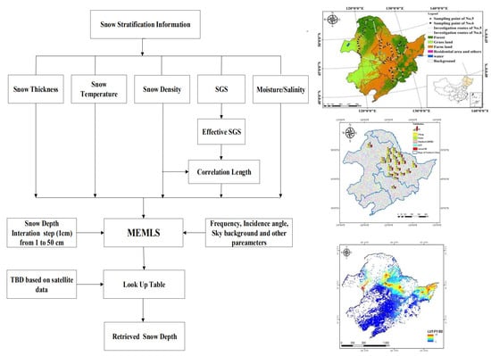
Accurate simulation of the TB of snowpacks using MEMLS requires prior information of snow parameters. According to the snow measurement results from the three snow investigations, each parameter can be empirically determined using the following strategies.

3.3.1. Snow Stratification

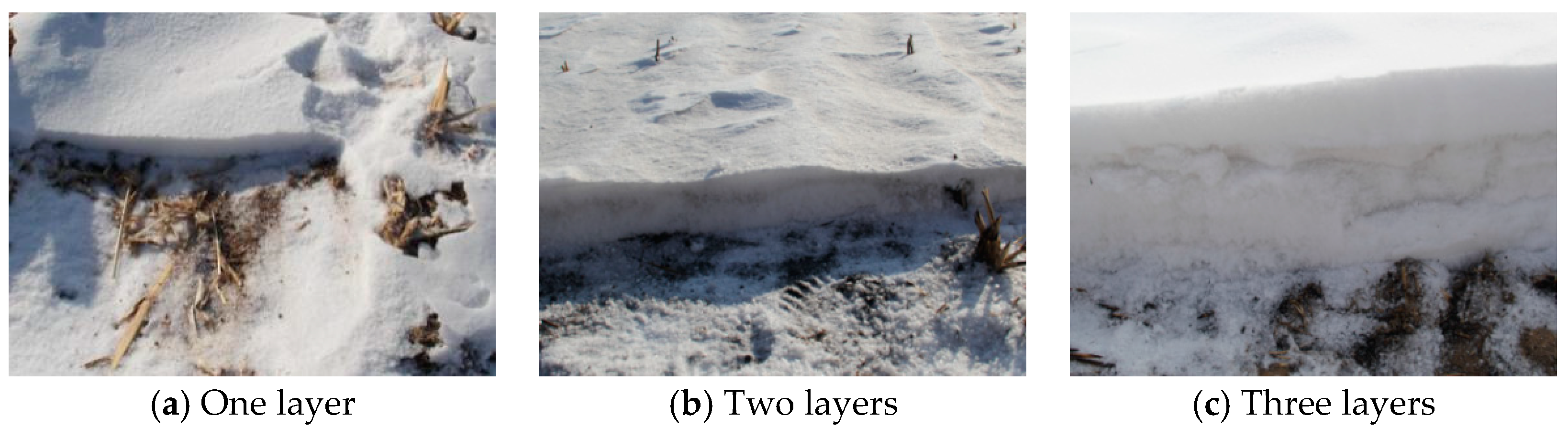
During the snowy season, new snowfalls continue to cover previous snowfalls, resulting in a gradual stratification of snow. Based on the field measurements in farmland, it was found that snow cover could be divided into three-layered snowpacks (Figure 4). SD and snow stratification mostly satisfied the following relationships: when SD was less than 7 cm, snow cover was not stratified and defined as one layer; when SD was 8–15 cm, snow cover was characterized as two layers, and the thickness of upper and bottom layer were assumed to be equal; when the actual SD exceeded 15 cm, the snow cover was divided into three layers. For the three-layer snowpacks, the same thickness was assumed for the upper and bottom snow layers. In the snow field measurements, it was found that the SD in Northeast China was never more than 50 cm, so an SD over 50 cm was not considered in this study.
The snow cover depth (SD) can be expressed as follows:
S D = i = 1 L a y e r N u m t h i c k n e s s ( i )
where LayerNum represents the number of snow layers and the thickness represents the thickness of each snow layer. Although in situ measurements of SD were not directly used in MEMLS, they are an important basis for determining the stratification of the snowpack. Based on the snow stratification information, the snow density, SGS, temperature, and other parameters of each layer were further measured. The measured SD was also recorded as the actual SD.

3.3.2. Snow Temperature

Snow temperature influences the retrieval of the SD to some extent. Generally, snow cover has a thermal insulation effect on the ground. The deeper the snow cover, the more obvious the thermal insulation effect [32]. According to the actual measurement results, the snow temperature is generally higher than the air temperature. For simplicity, in this study, snow temperatures (Tsnow) were determined by the following empirical equation:
T s n o w = s l o p e × S D + T a i r
where T
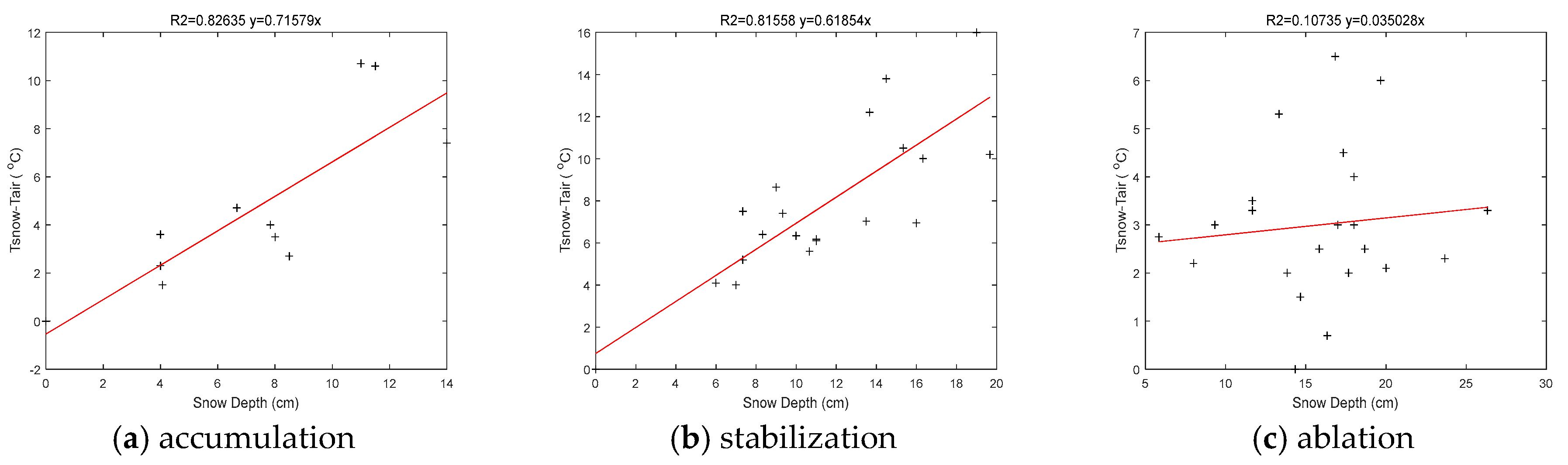
air represents air temperature in °C, SD represents snow depth in cm, slope represents the rate of change of snow temperature with SD which can be determined on the basis of the snow temperature and air temperature obtained from the measurement data. Thus, regression slopes in the three periods of snow accumulation, stabilization, and ablation were made.
As shown in Figure 5a,b, the snow temperature at the air/snow interface was assumed to be equal to the air temperature; thus, the difference between the air temperature and the snow temperature increases linearly with an increase in SD. The rate of change of the snow temperature slope gradually decreases with time, meaning that the difference between air temperature and snow temperature becomes smaller from snow accumulation to snow ablation. As shown in Figure 5c, the slope of Tsnow–Tair is relatively small, implying that there is little correlation between the difference of Tsnow and Tair and SD during ablation. By analysis, the correlation between air temperature and snow temperature was very high during the snow ablation period and, thus, the relationship between them can be established.
When the snow depth is greater than 25 cm, the snow temperature at the snow/soil interface tends to be stable due to the thermal insulation of a deep snowpack. Therefore, the snow temperature (Tsnow) can be computed from the air temperature (Tair) and snow depth (SD):
T s n o w = { 0.7 S D + T a i r i n a c c u m m u l a t i o n 0.6 S D + T a i r i n s t a b i l i z a t i o n 0.8 T a i r      i n a b l a t i o n

3.3.3. Snow Density

Commonly, the old bottom layer of snowpack generally has a larger SGS and a higher snow density due to compaction. By contrast, the fresh upper layer of snowpack generally has a smaller SGS and lower snow density. Table 2 describes the measured snow density of each layer from bottom to top during the three snowfall periods. From the accumulation period to the ablation period, the overall snow density tends to increase. In the accumulation period, only two-layer snowpacks exist and the snow density of the bottom layer is slightly higher than that of upper layer. In the stabilization and ablation period, the snow density of each layer is very similar. As a result, the snow density is almost equal in the three layers during the three periods, showing that the phenomenon of snow stratification is not evident in farmland.

3.3.4. Snow Grain Size

(A) SGS statistical results
The vertical temperature gradient of snow cover controls the deformation of dry snow. Because the saturated water vapor pressure is an exponential function of temperature, the temperature gradient inevitably leads to a certain gradient of water vapor pressure. The diffusion of water vapor from warm crystals to cold crystals leads to the destruction of warm crystals, and the reconstruction of crystal morphology at the cold end leads to the change of grain morphology and size, which causes the shape of snow grains to vary with time. As a result, the shape of snow particles gradually becomes spherical or cylindrical over time. Assuming the snow particles are pillars, we used the previously proposed automatic method for measuring and recording snow particle size [33]. This mainly utilizes digital image processing to find the outline of the SGS and avoids errors caused by manual measurement. As shown in the third column of Figure 6, the length and width of the red rectangle surrounding the snow particle was defined as the long and short sides of the particle, and the average result was used as the SGS of each layer.
Each layer of snow crystals includes different sizes. The grain size in a range of diameters was recorded, but the mean value was used for the whole layer. The scatterplots of the SGS values of each layer during different periods were analyzed to obtain the dynamic ranges of mean SGS, and the mean SGS values were taken as the representative values of each snow layer in a period. Table 3 describes the snow grain size variation with snow season. The SGS of each layer gradually increased over the snow season. In the vertical gradient of the snowpack, similar to snow density, SGS gradually decreases from the bottom layer to the upper layer.
(B) Improvement of SGS
According to the actual snow measurement, the snowpack is divided into three layers by natural stratification, and the snow parameters (i.e., snow density, SGS, and snow temperature) of each layer are measured. When simulating the TB of snowpacks using MEMLS, SGS is an important input parameter. In field investigations of SGS, it has been found that the depth hoar layer easily forms in the snow layer near to the ground. The SGS of a thick depth hoar layer was often larger than the upper layers, which resulted in a rapid decrease of simulated TBs, especially at 36 GHz frequency. If the measured SGS is directly input into the MEMLS to simulate the passive microwave TB, there is a deviation between the simulated TBs and TBs observed from satellite passive microwave sensors. Thus, this study proposed an effective SGS. Anna Kontu et al. [34] proposed an effective snow particle size to limit the growth of larger snow particle sizes and applied it in the HUT model. Similarly, in order to minimize the difference between the simulated TBs ( T B s i m ) and observed TBs ( T B o b s ) from satellite passive microwave sensors, we defined the optimal snow grain size ( D o p t ) as the free optimization parameter.
min | T B s i m ( D o p t ) T B o b s |
Considering the phenomenon of snow stratification was not evident in the farmland, we assumed that the SGS of each layer of snow was equal. Setting the SGS to vary from 0 to 5 mm with a 0.1 mm step, combined with the other measured parameters, the optimal snow grain size Dopt could be found that satisfied the simulated TBs based on the MEMLS that were closest to the observed TBs from satellite data.
Theoretically, the empirical coefficient of the effective SGS should be defined for each layer; however, this will lead to too many unknown parameters and underdetermined equations. Therefore, the measured layer thickness-weighted average SGS ( D a v e ) was first obtained using the following equation:
D a v e = i = 1 L a y e r N u m ( D i × d i ) / i = 1 L a y e r N u m d i
where LayerNum represents the number of snow layers, and Di and di represent the measured SGS and snow thickness of the ith layer, respectively.
The effective snow grain size ( D e f f ) could be obtained from D a v e .
D e f f = a × D a v e + b
For Equation (7), the parameters a and b can be obtained through the following minimization procedure:
M i n i = 1 n ( D e f f ( a , b ) D o p t ) 2
where n is the number of field measurement points during different snow observation periods. Finally, the empirical coefficients a and b are applied to each layer, and the effective SGS of each layer is obtained so that the SGS parameters and other snow parameters are matched and sent to the MEMLS.
From the viewpoint of satellite snow algorithms, an interesting factor is whether the difference TB18H − TB36H is modeled better than the individual channels. As analyzed in Section 5.3.3, generally, the root mean square error (RMSE) and Bias of the channel difference was lower and correlation was higher than those of the individual channels. As a result, the corresponding empirical coefficients fitted to simulate the channel difference for MWRI and AMSR2 in each period were retrieved using Equation (9) and are listed in Table 4. In general, the measured SGS in the snow ablation period was larger than the other periods; thus, the empirical coefficient a in the snow ablation was smaller than in the other periods. Using Equation (7), we computed the D e f f corresponding to each layer based on the empirical coefficients a and b , and further simulated the TBD between TB18 and TB36 based on MEMLS.

3.3.5. Correlation Length

Snow correlation length was defined to describe the influence of size and distribution of snow particles on scattering, which is related to snow density and SGS [35]. Therefore, snow density and SGS should be determined before estimating the correlation length. We first converted the snow density and the effective SGS to the correlation length, and further converted the correlation length to an exponential correlation length by multiplying by a constant (0.75) [36].
P e x = 0.75 ( 4 × ρ / ρ i × ( 1 ρ / ρ i ) / S )
where Pex represents the exponential correlation length, ρ represents the snow density, ρi represents the ice density (0.917 g/cm3), and S represents the surface area of the effective SGS per unit volume.
S = 2 × a / n
where a is the side length of the cubic box and n is the number of particles along its one side.
According to the field measurements, the particle form is similar to the pillar, so we used the calculated effective SGS as the long-side length and the short-side length was randomly selected to be between two-thirds and one times the long-side length. It was assumed that these numbers were homogeneously distributed within a cubic box, and the volume of the cubic box can be calculated according to snow density and the volume of particles [22]. Using Equation (10), the exponential correlation length can be calculated on the basis of the effective SGS range and snow density as presented in Table 5.

4. SD Retrieval Algorithm

4.1. Retrieved SD Based on LUT

Using the MEMLS physical model to directly retrieve SD is a complex process, not only because of the interrelationship between many input parameters but, also, the complexity of the physical model based on the radiative transfer equation. Chang et al. concluded that there is a linear relationship between SD and TBD [37,38,39,40,41], so we can obtain the TB from the MEMLS, and then establish the relationship between TBD and SD. Based on the statistical analysis results of the snow parameters (snow layers, snow density, SGS, and air temperature) measured in the field, in the process of applying the MEMLS, we assumed that the SD is unknown, and set a dynamic range for SD. According to each SD value in the range, we used the model to simulate TBs at 18 and 36 GHz, and further established a lookup table (LUT) between the TBD and the SD. LUT is a calculated array composed of TBD, SD, and other snow parameters. After using the above method to create an LUT, when the observed TB of the satellite passive microwave is known, the corresponding TBD can be obtained and, thus, the corresponding SD can be searched for from the LUT, given the other snow parameters. The snow parameters should be representative of the region so that the LUT built by inputting these parameters into the model can be well applied.
Based on the snow stratification information of farmland from the snow survey of Northeast China, MEMLS was used to establish LUT for three cases of layering, namely, a one-layer LUT established for an SD of 5–7 cm, a two-layer LUT for an SD of 8–15 cm, and a three-layer LUT for an SD of more 15 cm. After analyzing snow statistical information, the corresponding snow property parameters of each layer in the three periods described in previous sections were input and a dynamic range (1–50 cm) for the SD variable with an interval of 1 cm was set. The corresponding TB at 18 and 36 GHz at the H-POL were simulated using MEMLS. Furthermore, the simulated TBD was obtained by calculating the difference in TB data between 18 and 36 GHz. Thus, the relationship between the snow properties and the simulated TBD can be established in the LUT. When retrieving SD based on the established LUT, the observation TBD needed to first be calculated from the satellite passive microwave data. Then, combining the TBD with the snow observation date, air temperature, and other reference information, the SD could be retrieved by searching the position where the observed TBD was closest to the simulated TBD.

4.2. Empirical SD Retrieval Algorithm

The instrument designed parameters of SSMIS, AMSR2, and MWRI radiometer are very similar [37,38,39,40]. Therefore, we make a comparison of these following methods for both AMSR2 and MWRI data in the study area.
(A) Chang’s Algorithm
Using Chang’s algorithm [41] and assuming that snow was homogeneous, the dry snow density was 0.3 g/cm3, and the SGS was 0.3 mm in diameter. The following algorithm was applicable:
S D = C × ( T b 18 H T b 37 H )
where S D represents snow depth (cm), the retrieval coefficient C was 1.59, and T B 18 H and T B 37 H were, respectively, 18 and 37 GHz data at H-POL.
(B) Foster’s Algorithm
Foster et al. [42] refined the retrieval coefficient of Chang’s algorithm. When the SGS is 0.4 mm in diameter, the retrieval coefficient becomes 0.78 and the refined algorithm is then
S D = 0.78 × ( T b 18 H T b 37 H ) .
(C) Standard AMSR2 Algorithm
The current AMSR2 SD algorithm is an evolution of the original AMSR-E SWE algorithm and takes advantage of the channels 10, 18, 23, 36, and 89 GHz available on the AMSR-E. The application of this algorithm is described in [43,44].
(D) Standard MWRI Algorithm
The land surface is divided into four types: grassland, farmland, bare ground, and forest. For each grid cell, the SD is estimated from the sum of SD values from each land cover algorithm, weighted by the percentage of the land cover type within each grid cell. The application of this algorithm is described in [45,46].

5. Results and Analysis

5.1. Retrieval Results

MWRI and AMSR2 data during the period of the snow survey were collected to retrieve the SD. According to the latitude and longitude information of the sampling points, the nearest neighbor search algorithm is used to find the passive microwave pixels covering the sampling points. The SD data of the sampling points represented the actual SDs of the corresponding microwave pixels. Combining the observed TBD calculated at 18 and 36 GHz at H-POL from satellite data, the SD based on the statistical LUTs was obtained and further compared with the retrieval SDs by Chang’s algorithm, Foster’s algorithm, the standard MWRI algorithm, and the standard AMSR2 algorithm, as well as the measured SDs along the snow course. In the proposed method, half of the measured snow parameter data are used to establish the LUT and half are used to verify the LUT. The SD retrieval results of different algorithms are shown in Figure 7. Moreover, the difference between the SD retrieval result of each algorithm and the actual SD (DSD) was calculated, and the absolute values of the DSD results are shown in Figure 8. For MWRI data, the SD retrieval results based on the statistical LUT, Foster’s algorithm, and standard MWRI algorithm are closer to the actual SD, while the retrieval results obtained using Chang’s algorithm had larger errors. For the AMSR2 data, the SD retrieval results based on the statistical LUT and Foster’s algorithm were closer to the actual SD, while the retrieval results based on Chang’s algorithm and the standard AMSR2 algorithm had larger errors.

5.2. Result Analysis

The RMSE and Bias selected to evaluate the retrieval precision of the SD calculated by these algorithms can be expressed as follows:
R M S E = 1 n i = 1 n ( N i M i ) 2
B i a s = 1 n i = 1 n ( N i M i )
where n is the number of field measurement points of the SD, Ni represents the retrieval result of the SD, and Mi is the actual SD.
Table 6 and Table 7 show the RMSE and Bias values calculated using the measured SD along with the retrieval results of the SD for MWRI and AMSR2 obtained using the four algorithms. As listed in Table 5 and Table 6, the following can be seen:
(1)
During the snow accumulation period, because the snow on the farmland was relatively shallow and many sampling points were not covered with snow, there were fewer sampling points than during the other two periods. For MWRI data, Chang’s algorithm overestimates SD, while the other three algorithms were close to the measured SD. The SD results using the statistical LUT had the highest retrieval accuracy, followed by Foster’s algorithm, and then the standard MWRI algorithm. For AMSR2 data, both Chang’s algorithm and the standard AMSR2 algorithm overestimated SD. The retrieval results of SD using the statistical LUT achieved higher retrieval precision than Foster’s algorithm.
(2)
During the snow stabilization period, snow parameters were more representative because of relatively stable snow conditions. For MWRI and AMSR2 data, Chang’s algorithm still overestimated SD, similar to that in the snow accumulation period. The statistical LUT algorithm SD retrieval accuracy for both MWRI and AMSR2 data was higher than that of all the other algorithms. The standard MWRI algorithm performs well for MWRI data, but the standard AMSR2 algorithm for AMSR2 greatly overestimated SD. The SD retrieval accuracy using Foster’s algorithm was slightly less than it was during the snow accumulation period.
(3)
During the snow ablation period, due to higher air temperature on several days, snow melted and condensed, which caused the SD retrieval results based on passive microwave data to differ from the measured SD. The retrieval result of the statistical LUT algorithm was the closest to the actual SD, followed by that of the standard MWRI algorithm, then Foster’s algorithm. Chang’s algorithm and standard AMSR2 algorithm again had the worst SD retrieval accuracy.
The standard deviation of DSD based on sampling points was calculated, which is described in Table 8. From Table 8, the STD results using LUT are the lowest of the four SD retrieval algorithms, which means that LUT can better reflect the spatial distribution of actual SD in the area compared to the other algorithms.
Standard deviation S T D is calculated by
STD = 1 n i = 1 n ( N i μ ) 2
where N i is the difference of actual SD and retrieval SD (DSD) of the ith sampling point, and μ is the average DSD.

5.3. Discussion

5.3.1. SD Spatial Variability

When we designed the snow parameters investigation route, we took the footprint of the passive microwave pixel into account and conducted the test on the representative sampling points in the passive microwave pixel. As shown in Figure 9, the color background grid in the figure represents a 10 km × 10 km passive microwave pixel. It can be seen from the distribution range of sampling points that the whole snow investigation range is large, including the main farmland areas in Northeast China. Combined with many years of snow field observation experience, the underlying surface of farmland in Northeast China is considered as uniform and flatly distributed. Thus, the variation of farmland SD in each microwave pixel is small, so the sampling point data is representative. It can also be seen from the figure that the snow condition distribution in Northeast China increases gradually with increasing latitude. The SD in this area increases gradually with increasing latitude. In addition to Chang’s algorithm, the SD results of other algorithms is similar to the actual SD, which demonstrates that the empirical coefficient of Chang’s algorithm is not suitable for this area. The SGS and snow density in the study area are quite different from the snow parameter conditions applied by Chang’s algorithm. In the process of establishing the standard MWRI algorithm, a large number of meteorological station data in China were selected, so the retrieval accuracy of SD in this area is higher than that of the standard AMSR2 algorithm. Compared with other algorithms, in terms of spatial distribution and snow cover accuracy, SD retrieval results using the LUT for the two types of data are closest to the actual snow cover survey results in each period, indicating that this method can be used for multisource passive microwave radiation data and has good potential for application in high-precision SD retrieval in local observation areas.
Due to the large amount of data in the whole observation period, the data of 27 January 2018 is taken as an example to demonstrate the farmland SD in Northeast China. As shown in the Figure 10 and Figure 11, the LUT algorithm provides an effective method to obtain high-precision SD distribution in farmland.

5.3.2. SD Temporal Variability

The box plots in Figure 12 show the mean values and ranges of the SD results in the study area. A box plot is a statistical chart that displays the spread of a dataset. It is mainly used to reflect the distribution characteristics of the original data and can also compare the distribution characteristics of multiple groups of data. The drawing method of a box line graph is to determine the maximum, minimum, median, and quartiles of a set of data, then to draw the box by connecting two quartiles, and finally to connect the maximum and minimum with the box, with the median in the middle of the box. As shown in Figure 12, the actual SD is relatively stable for the whole snow season, with the SD range varying around the mean value. For both MWRI and AMSR2 data, the SD retrieval accuracy of the statistical LUT algorithm is overall superior to the other algorithms due to the fact that its SD change trend is more similar to that of the actual SD. For Chang’s algorithm, the range of the SD retrieval results varied dramatically, which caused larger SD retrieval errors. When applying the same algorithm to passive microwave data of a particular satellite, for example, the statistical LUT algorithm, Foster’s algorithm, or Chang’s algorithm, the SD retrieval results based on MWRI data are slightly better than those based on AMSR2 data. In addition, the standard MWRI algorithm was demonstrated to perform well for MWRI data, in contrast to the standard AMSR2 algorithm, which seemed to be ineffective when applied to the AMSR2 data in the study area. Foster’s algorithm obtained more accurate SD results in the snow accumulation period, but in the other two periods, the range obtained using this algorithm contained obvious bias compared to the actual SD.
In summary, the SD retrieval results obtained using the statistical LUT algorithm achieved the highest accuracy for the study area because the algorithm fully considers the variation in snow property parameters during different snow periods. The standard MWRI algorithm also performed well for MWRI data throughout the whole snow season. The SD retrieval results obtained using Foster’s algorithm were far better than those obtained using Chang’s algorithm, indicating that the snow density and SGS applied in Foster’s algorithm were more suitable for the study area. However, snow conditions continually change throughout the whole snow season and using constant snow property parameters in the traditional empirical SD retrieval algorithms decreases the retrieval accuracy.

5.3.3. Solution of the Effective SGS

The effect of SGS was analyzed by minimizing the error of the simulated TB and observed TB with Equation (6). During the snow stabilization period, the snowpack was relatively stable and the most measured SGS data were obtained. Thus, the simulated TB from the MEMLS model versus the observed TB from the MWRI and AMSR2 algorithms in this period is taken as an example. The correlations (r), biases (Bias), and root mean squared errors (RMSE) between the simulated and observed data were also computed. The scatterplots of those results in 18 and 36 GHz at H-POL, as well as their difference (TB18H − TB36H), are shown in Figure 13 and Figure 14, respectively. For the MWRI and AMSR2 data, the correlations are the highest and the RMSE and Bias are the lowest in the observed and simulated channel differences over the individual channels. The effective SGS listed in Equations (17) and (18) can correctly predict the channel difference for MWRI and AMSR2 data, respectively.
D e f f _ M W R I = 0.51 D a v e + 0.11
D e f f _ A M S R 2 = 0.57 D a v e 0.02

5.3.4. Error Analysis

Errors are mainly from measurement and statistical data processing. The measurement errors are generally caused by the instrument itself or operational issues during the investigation. For example, errors occur in the results of the snow fork in cold temperatures. The measurement of SGS is only carried out on two-dimensional images of SGS photos, and the processed results cannot represent the actual SGS distribution. In addition, snow parameters including temperature, density, and SGS were processed through statistical analysis, which would contain some errors in the simulation of the TB when applying the MEMLS. In the establishment of the LUT, the layered snow temperature was obtained on the basis of the SD and a linear relationship between the difference in temperature at the snow/soil interface and the air temperature. However, when the air temperature increases rapidly due to the insulating effect of snow, the air temperature will be higher than the snow temperature. The increase in the temperature at the snow/soil interface to the underlying ground may not be linear, which could result in uncertainty in temperature at some snow layers. In addition, in order to obtain the effective SGS, it was assumed that the SGS of all layers of farmland snow was the same, which would also bring about some errors.

6. Conclusions

In Northeast China, agriculture is the main source of production, and snow plays an important role in crop growth. In this paper, through the statistical analysis of snow parameters and environmental parameters measured in the three periods of snow accumulation, stabilization, and ablation, the TB time series of snow-covered farmland in varying snow periods was simulated using MEMLS. The TBD data computed from the observed MWRI and AMSR2 data were used to find the SD from the established LUT. Furthermore, the SD retrieval results were compared with the actual SD and the SD retrieved by Chang’s algorithm, Foster’s algorithm, the standard MWRI algorithm, and the standard AMSR2 algorithm. The experimental results demonstrated that the statistical LUT achieved higher SD retrieval accuracy than the other algorithms. In the whole snow season, the average RMSE of SD was approximately 3.97 and 4.22 cm, while the average Bias of SD was 3.12 and 3.52 cm for MWRI and AMSR2 data, respectively. The experimental results show that the proposed method provides an effective method to obtain high-precision SD in farmland. This method has a strong potential for use in snow observation in agricultural areas and serving for local application.
At present, the commonly used SD retrieval methods have their own adaptive conditions. For example, the Chang algorithm was developed in Siberia, while the Foster algorithm refined the empirical coefficient of Chang’s algorithm for larger SGS and considered forest cover influence. The AMSR-E algorithm takes advantage of multiple channels. The MWRI algorithm considers the influence of the mixed pixel of the underlying surface. Most of the algorithms give good results for global SD retrieval, but there are still biases in local SD retrieval. The LUT is established by combining the statistical analysis of the snow parameter data with MEMLS. The advantage of this method is that once the LUT is established, it can find the SD according to the TBD of the satellite passive microwave. SD research of a local observation area has better applicability as compared with other existing SD retrieval algorithms.
MEMLS is quite reliable when applied to different satellite-borne microwave radiometer data when the statistical results of prior snow parameters of each period are available. The simulations with limited in situ data showed that snow temperature, snow density, and SGS have a great impact on the simulation accuracy of TB. To ensure the stability of the simulation results of TB from MEMLS, the input snow properties parameters should represent the average situation of the observation area. Considering the measured data mainly covered a pure farmland land cover type under the Instantaneous Field Of View (IFOV) of satellite passive microwave sensors, the statistical values of the snow parameters were input to MEMLS; furthermore, the statistical LUTs for the three snow periods were established. Considering larger SGS would cause higher error when simulating TB, a time series of the effective SGS was calculated by minimizing the simulation error between the simulated TB and the observed TB. It was also found that the simulation with the effective SGS as an input to model the channel difference between TB18 and TB37 had a lower RMSE and a higher correlation with the observed satellite data than each individual channel, which are often used in remote sensing of snow. The SD retrieval algorithm based on the statistical LUT utilizing snow characteristics can improve the accuracy of SD estimation from satellite passive microwave data, thereby improving monitoring capabilities of SD in farmland for the whole snow season. The experimental results show that this method can effectively combine the MEMLS physical model with satellite remote sensing data and obtain the snow parameters of the observation area by an LUT. If there is field data in other areas and at other times, the method can also be applied to other passive microwave TB data.

Author Contributions

All authors have read and agree to the published version of the manuscript. Conceptualization, L.G.; methodology, L.G. and X.F.; software, L.G. and X.F.; validation, L.G. and X.F.; formal analysis, L.G. and X.L.; investigation, X.F. and Y.W.; resources, L.G.; data curation, L.G. and X.F.; writing—original draft preparation, L.G.; writing—review and editing, L.G.; visualization, L.G.; supervision, L.G.; project administration, L.G.; funding acquisition, L.G.

Funding

This research was funded by National Natural Science Foundation of China, grant number 41871225.

Acknowledgments

This work was supported in part by the National Natural Science Foundation of China under Grant 41871225 and Basic Resources Survey Project of National Science and Technology—The investigations on the characteristics and distribution of snow in China. We also thank Science and Technology Basic Resources Survey Project of China for providing snow test data for this study.

Conflicts of Interest

The authors declare no conflicts of interest.

References

  1. Robinson, D.A.; Dewey, K.F.; Heim, R.R. Global Snow Cover Monitoring: An Update. Bull. Am. Meteorol. Soc. 1993, 74, 1689–1696. [Google Scholar] [CrossRef] [Green Version]
  2. Clifford, D. Global estimates of snow water equivalent from passive microwave instruments: History, challenges and future developments. Int. J. Remote Sens. 2010, 31, 3707–3726. [Google Scholar] [CrossRef]
  3. Shi, J.; Xiong, C.; Jiang, L. Review of snow water equivalent microwave remote sensing. Sci. Sin. Terrae 2016, 46, 529–543. [Google Scholar] [CrossRef]
  4. Rott, H.; Sturm, K. Microwave signature measurements of Antarctic and Alpine snow. In Proceedings of the 11th EARSeL Symposium, Graz, Austria, 3–5 July 1991; pp. 140–151. [Google Scholar]
  5. Foster, J.L.; Hall, D.K.; Chang, A.T.C. An overview of passive microwave snow research and results. Rev. Geophys. 1984, 22, 195–208. [Google Scholar] [CrossRef]
  6. Derksen, C.; Walker, A.; Ledrew, E. Combining SMMR and SSM/I data for time series analysis of central north American snow water equivalent. J. Hydrometeorol. 2003, 4, 304–316. [Google Scholar] [CrossRef]
  7. Kawanishi, T. The advanced microwave scanning radiometer for the earth observing system (AMSR-E), NASDA’s contribution to the EOS for global energy and water cycle studies. IEEE Trans. Geosci. Remote Sens. 2003, 41, 184–194. [Google Scholar] [CrossRef]
  8. Hu, Y.; Jian-Cheng, S. On the estimation of land surface parameters by using FY-3A Microwave Radiometer Imager (MWRI). Remote Sens. Technol. Appl. 2005, 20, 194–200. [Google Scholar]
  9. Cho, E.; Tuttle, S.E.; Jacobs, J.M. Evaluating consistency of snow water equivalent retrievals from passive microwave sensors over the north central U. S.: SSM/I vs. SSMIS and AMSR-E vs. AMSR2. Remote Sens. 2017, 9, 465. [Google Scholar]
  10. Kelly, R. The AMSR-E snow depth algorithm: Description and initial results. J. Remote Sens. Soc. Jpn. 2009, 29, 307–317. [Google Scholar]
  11. Chang, A.T.C.; Foster, J.L.; Hall, D.K. Effects of forest on the snow parameters derived from microwave measurements during the BOREAS winter field experiment. Hydrol. Process. 1996, 10, 1565–1574. [Google Scholar] [CrossRef]
  12. Foster, J.L.; Chang, A.T.C.; Hall, D.K. Comparison of snow mass estimates from prototype passive microwave snow algorithm, a revised algorithm and snow depth climatology. Remote Sens. Environ. 1997, 62, 132–142. [Google Scholar] [CrossRef]
  13. Wiesmann, A.; Mätzler, C. Microwave emission model of layered snowpacks. Remote Sens. Environ. 1999, 70, 307–316. [Google Scholar] [CrossRef]
  14. Picard, G.; Brucker, L.; Roy, A.; Dupont, F.; Fily, M.; Royer, A.; Harlow, C. Simulation of the microwave emission of multi-layered snowpacks using the dense media radiative transfer theory: The DMRT-MLmodel. Geosci. Model. Dev. 2013, 6, 1061–1078. [Google Scholar] [CrossRef] [Green Version]
  15. Tsang, L.; Chen, C.T.; Chang, A.T.C.; Guo, J.; Ding, K.H. Dense media radiative transfer theory based on quasicrystalline approximation with applications to passive microwave remote sensing of snow. Radio Sci. 2000, 35, 731–749. [Google Scholar] [CrossRef]
  16. Chang, W.; Tan, S.; Lemmetyinen, J.; Tsang, L.; Xu, X.; Li, X.; Yueh, S. Dense media radiative transfer applied to SnowScat and SnowSAR. IEEE J. Sel. Top. Appl. Earth Obs. Remote. Sens 2014, 7, 3811–3825. [Google Scholar] [CrossRef]
  17. Lemmetyinen, J.; Pulliainen, J.; Rees, A.; Kontu, A.; Qiu, Y.; Derksen, C. Multiple layer adaptation of the HUT snow emission model: Comparison with experimental data. IEEE Trans. Geosci. Remote Sens. 2010, 48, 2781–2794. [Google Scholar] [CrossRef]
  18. Mätzler, C.; Wiesmann, A. Extension of the microwave emission model of layered snowpacks to coarse-grained snow. Remote Sens. Environ. 1999, 70, 317–325. [Google Scholar] [CrossRef]
  19. Royer, A.; Roy, A.; Montpetit, B. Comparison of commonly-used microwave radiative transfer models for snow remote sensing. Remote Sens. Environ. 2017, 190, 247–259. [Google Scholar] [CrossRef] [Green Version]
  20. Che, T.; Dai, L.Y.; Zheng, X.M. Estimation of snow depth from passive microwave brightness temperature data in forest regions of northeast China. Remote Sens. Environ. 2016, 183, 334–349. [Google Scholar] [CrossRef]
  21. Che, T.; Dai, L.; Wang, J. Estimation of snow depth and snow water equivalent distribution using airborne microwave radiometry in the Binggou Watershed, the upper reaches of the Heihe River basin. Int. J. Appl. Earth Obs. Geoinf. 2012, 17, 23–32. [Google Scholar] [CrossRef]
  22. Dai, L.; Che, T.; Wang, J. Snow depth and snow water equivalent estimation from AMSR-E data based on a priori snow characteristics in Xinjiang, China. Remote Sens. Environ. 2012, 127, 14–29. [Google Scholar] [CrossRef]
  23. Gu, L.J.; Ren, R.Z.; Li, X.F. Snow depth retrieval based on a multi-frequency dual-polarized passive-microwave unmixing method from mixed forest observations. IEEE Trans. Geosci. Remote Sens. 2016, 54, 1–13. [Google Scholar] [CrossRef]
  24. Wang, J.; Feng, X.; Xiao, P.; Ye, N.; Zhang, X.; Cheng, Y. Snow grain-size estimation over mountainous areas from modis imagery. IEEE Geosci. Remote Sens. Lett. 2018, 15, 97–101. [Google Scholar] [CrossRef]
  25. Wu, L.; Li, X.; Zhao, K.; Zheng, X.; Jiang, T. Brightness temperature simulation of snow cover based on snow grain size evolution using in situ data. J. Appl. Remote Sens. 2016, 10, 036016. [Google Scholar] [CrossRef]
  26. Tanikawa, T.; Hori, M.; Aoki, T.; Hachikubo, A.; Stamnes, K. In situ measurements of polarization properties of snow surface under the brewster geometry in hokkaido, japan and northwest greenland ice sheet. J. Geophys. Res. Atmos. 2014, 119, 13–964. [Google Scholar] [CrossRef]
  27. Gu, L.J.; Zhao, K.; Zhang, S.W.; Zhang, S. Comparative analysis of microwave brightness temperature data in Northeast China using AMSR-E and MWRI products. Chin. Geogr. Sci. 2011, 21, 84–93. [Google Scholar] [CrossRef]
  28. Yang, H.; Weng, F.Z.; Lv, L.Q.; Lu, N.M. The FengYun-3 microwave radiation imager on-orbit verification. IEEE Trans. Geosci. Remote Sens. 2011, 49, 4552–4560. [Google Scholar] [CrossRef]
  29. Pan, J.; Durand, M.; Sandells, M. Differences between the HUT snow emission model and MEMLS and their effects on brightness temperature simulation. IEEE Trans. Geosci. Remote Sens. 2016, 54, 2001–2019. [Google Scholar] [CrossRef]
  30. Wu, L.; Li, X.; Zhao, K.; Zheng, X. Snow depth inversion using the localized hut model based on FY-3b MWRI data in the farmland of heilongjiang province, China. J. Indian Soc. Remote Sens. 2017, 45, 89–100. [Google Scholar] [CrossRef]
  31. Qiu, Y.B.; Shi, J.C.; Lemmetyinen, J.; Kontu, A.; PuIiainen, J.; Guo, H.D. The atmosphere inflfluence to AMSR-E measurements over snow-cover areas: Simulation and experiments. IEEE Trans. Geosci. Remote Sens. 2010, 2, 610–613. [Google Scholar]
  32. Tsutsui, H.; Koike, T.; Graf, T. Development of a dry-snow satellite algorithm and validation at the CEOP reference site in Yakutsk. J. Meteorol. Soc. Jpn. 2007, 85A, 417–438. [Google Scholar] [CrossRef] [Green Version]
  33. Fan, X.; Gu, L.; Ren, R. Automatic snow grain size measurement method based on adaptive minimum circumscribed rectangle. In Proceedings of the Frontiers in Optics, Washington, DC, USA, 16–20 September 2018; Optical Society of America: Washington, DC, USA, 2018; p. JW4A-130. [Google Scholar]
  34. Kontu, A.; Pulliainen, J. Simulation of spaceborne microwave radiometer measurements of snow cover using in situ data and brightness temperature modeling. IEEE Trans. Geosci. Remote Sens. 2010, 48, 1031–1044. [Google Scholar] [CrossRef]
  35. Pulliainen, J.T.; Grandell, J.; Hallikainen, M.T. HUT snow emission model and its applicability to snow water equivalent retrieval. IEEE Trans. Geosci. Remote Sens. 1999, 37, 1378–1390. [Google Scholar] [CrossRef]
  36. Mätzler, C. Relation between grain-size and correlation length of snow. J. Glaciol. 2002, 48, 421–466. [Google Scholar] [CrossRef] [Green Version]
  37. Lv, X.; Gong, A.; Yin, X.; Li, J.; Chen, Y. Inter-calibration of satellite passive microwave land observations from MWRI and AMSR-E over the bare soil and grassland. In Proceedings of the IGARSS 2016—2016 IEEE International Geoscience and Remote Sensing Symposium, Beijing, China, 10–15 July 2016. [Google Scholar]
  38. Jinyang, D.; John, K.; Jiancheng, S.; Lucas, J.; Shengli, W.; Ruijing, S. Inter-calibration of satellite passive microwave land observations from amsr-e and amsr2 using overlapping fy3b-mwri sensor measurements. Remote Sens. 2014, 6, 8594–8616. [Google Scholar]
  39. Yang, H.; Lv, L.Q.; Xu, H.X.; He, J.K. Evaluation of FY3B-MWRI instrument on-orbit calibration accuracy. In Proceedings of the IEEE International Conference on Geoscience and Remote Sensing Symposium, Vancouver, BC, Canada, 24–29 July 2011; pp. 2252–2254. [Google Scholar]
  40. Wu, S.; Chen, J. Instrument performance and cross calibration of FY-3C MWRI. In Proceedings of the IGARSS 2016—2016 IEEE International Geoscience and Remote Sensing Symposium, Beijing, China, 10–15 July 2016. [Google Scholar]
  41. Chang, A.T.C.; Foster, J.L.; Hall, D.K. Nimbus-7 SMMR derived global cover parameters. Ann. Glaciol. 1987, 9, 39–44. [Google Scholar] [CrossRef] [Green Version]
  42. Foster, J.L.; Hall, D.K.; Kelly, R.E.J.; Chiu, L. Seasonal snow extent and snow mass in South America using SMMR and SSM/I passive microwave data (1979–2006). Remote Sens. Environ. 2009, 113, 291–305. [Google Scholar] [CrossRef] [Green Version]
  43. Zhang, R.P.; Liang, T.G.; Feng, Q.S.; Huang, X.D.; Wang, W.; Xie, H.J.; Guo, J. Evaluation and Adjustment of the AMSR2 Snow Depth Algorithm for the Northern Xinjiang Region, China. IEEE J. Sel. Top. Appl. Earth Obs. Remote Sens. 2016, 99, 1–12. [Google Scholar] [CrossRef]
  44. Gu, L.J.; Ren, R.Z.; Li, X.F.; Zhao, K. Snow Depth retrieval based on a multifrequency passive microwave unmixing method for saline-alkaline land in the western Jilin province of China. IEEE J. Sel. Top. Appl. Earth Obs. Remote Sens. 2018, 11, 2210–2222. [Google Scholar] [CrossRef]
  45. Jiang, L.; Wang, P.; Zhang, L.X. Improvement of snow depth retrieval for FY3B-MWRI in China. Sci. China Earth Sci. 2014, 57, 1278–1292. [Google Scholar] [CrossRef]
  46. Gu, L.J.; Ren, R.Z.; Zhao, K.; Li, X.F. Snow depth and snow cover retrieval from FengYun3B microwave radiation imagery based on a snow passive microwave unmixing method in Northeast China. J. Appl. Remote Sens. 2014, 8, 084682. [Google Scholar] [CrossRef]
Figure 1. Study area, located in Northeast China, including the land cover distribution and the snow investigation routes of the survey project.
Remotesensing 11 03037 g001
Figure 2. Investigation instruments in the snow survey.
Remotesensing 11 03037 g002
Figure 3. SD retrieval algorithm based on the lookup table (LUT) built from microwave emission model of layered snowpacks (MEMLS).
Remotesensing 11 03037 g003
Figure 4. Snow stratification in farmland.
Remotesensing 11 03037 g004
Figure 5. Relationship between snow depth (SD) and air and snow temperature differences.
Remotesensing 11 03037 g005
Figure 6. Comparisons of the measurement results of snow grain size (SGS) (using 1 mm grid).
Remotesensing 11 03037 g006
Figure 7. Actual SD and SD retrieval results using the four algorithms in farmland (the left side of the dividing line of the horizontal axis being the input data and the right side being the verification data).
Remotesensing 11 03037 g007
Figure 8. Comparison of DSD results using different retrieval algorithms (the left side of the dividing line of the horizontal axis being the input data and the right side being the verification data).
Remotesensing 11 03037 g008
Figure 9. Comparison of retrieval SD and actual SD at the samples for MWRI data in the (a) accumulation (c) stabilization, and (e) ablation period and AMSR2 data in the (b) accumulation, (d) stabilization, and (f) ablation period.
Remotesensing 11 03037 g009
Figure 10. Comparison of farmland SD results using MWRI data and different retrieval algorithms in Northeast China.
Remotesensing 11 03037 g010
Figure 11. Comparison of farmland SD results using AMSR2 data and different retrieval algorithms in Northeast China.
Remotesensing 11 03037 g011
Figure 12. Box plots of the SD retrieval results obtained using different algorithms in the three periods (the first and the second rows display the results of MWRI and AMSR2, respectively).
Remotesensing 11 03037 g012
Figure 13. MWRI observed TB versus simulated TB on bias, RMSE, and correlations using the effective SGS with Equation (16) (a) 18.7 GHz, (b) 36.5 GHz, and (c) channel difference 18.7 − 36.5 GHz on horizontal polarization.
Remotesensing 11 03037 g013
Figure 14. AMSR2 observed TB versus simulated TB on Bias, RMSE, and correlations using the effective SGS with Equation (17) (a) 18.7 GHz, (b) 36.5 GHz, and (c) channel difference 18.7 − 36.5 GHz on horizontal polarization.
Remotesensing 11 03037 g014
Table 1. Instrument specifications of passive microwave sensors.
FY3B-MWRICenter Frequency (GHz) 10.6518.723.836.589
Band Width (MHz) 1802004009002300
Polarization Type V, HV, HV, HV, HV, H
Instantaneous Field Of View (IFOV) (km × km) 51 × 8530 × 5027 × 4518 × 309 × 15
AMSR2Center Frequency (GHz)6.9/7.310.718.723.836.589
Band Width (MHz)35010020040010003000
Polarization TypeV, HV, HV, HV, HV, HV, H
IFOV (km × km)35 × 6224 × 4214 × 2215 × 267 × 123 × 5
Table 2. Statistical results of snow density (g/cm3) in farmland.
PeriodThree-Layer
BottomMiddleUpper
RangeMeanRangeMeanRangeMean
Accumulation0.089–0.1540.114\\0.058–0.1090.090
Stabilization0.086–0.2180.1280.105–0.1690.1290.058–0.1970.104
Ablation0.092–0.1970.1400.067–0.2380.1410.040–0.2550.135
Table 3. Statistical average SGS result (mm).
PeriodThree Layers
BottomMiddleUpper
RangeMeanRangeMeanRangeMean
Accumulation 2.46–3.112.82\\1.06–3.612.16
Stabilization 1.55–4.403.371.70–3.232.701.26–3.582.56
Ablation 1.44–6.004.441.60–5.123.911.04–4.573.10
Table 4. Empirical coefficients of effective SGS.
PeriodMWRIAMSR2
abab
Accumulation0.460.50.231.15
Stabilization0.510.110.57−0.02
Ablation0.240.810.181.07
Table 5. Exponential correlation length of the effective SGS.
Snow Density (g/cm3)Effective SGS (mm)
1.6–1.71.7–1.81.8–1.91.9–2.02.0–2.12.1–2.22.2–2.32.3–2.42.4–2.5
0.05–0.100.0990.1030.1070.110.1140.1180.1210.1250.129
0.10–0.150.1480.1540.1590.1650.1710.1760.1820.1870.192
0.15–0.200.1820.1890.1960.2030.210.2170.2230.230.236
0.20–0.250.2060.2140.2220.230.2380.2450.2530.260.268
0.25–0.300.2220.2310.240.2480.2570.2650.2730.2810.289
Table 6. Comparison of RMSE results obtained using the four SD retrieval algorithms.
MWRIAMSR2
AccumulationStabilizationAblationAccumulationStabilizationAblation
RMSE (cm)LUT3.314.234.363.394.744.53
Chang10.0325.4024.4311.0622.6422.71
Foster3.896.926.035.036.314.70
Standard4.495.005.6110.0216.7915.96
Table 7. Comparison of Bias results obtained using the four SD retrieval algorithms.
MWRIAMSR2
AccumulationStabilizationAblationAccumulationStabilizationAblation
Bias (cm)LUT2.353.333.682.654.003.92
Chang7.7822.8322.328.1819.5120.56
Foster3.065.274.934.424.803.47
Standard3.754.024.956.0514.1014.52
Table 8. Comparison of STD results obtained using the four SD retrieval algorithms.
MWRIAMSR2
AccumulationStabilizationAblationAccumulationStabilizationAblation
STD (cm)LUT2.322.602.352.122.542.27
Chang6.3311.129.917.4411.489.64
Foster2.414.483.462.394.083.17
Standard2.482.962.647.999.116.62

