Abstract
Currently, the accurate estimation of the maximum snow water equivalent (SWE) in mountainous areas is an important topic. In this study, in order to improve the accuracy and spatial resolution of SWE reconstruction in alpine regions, the Sentinel-2(MSI) and Landsat 8(OLI) satellite data with the spatial resolution of tens of meters are used instead of the Moderate-resolution Imaging Spectroradiometer (MODIS) data so that the pixel mixing problem is avoided. Meanwhile, geostationary satellite-based and topographic-corrected incoming shortwave radiation is used in the restricted degree-day model to improve the accuracy of radiation inputs. The seasonal maximum SWE accumulation of a river basin in the winter season of 2017–2018 is estimated. The spatial and temporal characteristics of SWE at a fine spatial and temporal resolution are then analyzed. And the results of reconstruction model with different input parameters are compared. The results showed that the average maximum SWE of the study area in 2017–2018 was 377.83 mm and the accuracy of snow cover, air temperature and the radiation parameters all affects the maximum SWE distribution on magnitude, elevation and aspect. Although the accuracy of other forcing parameters still needs to be improved, the estimation of the local maximum snow water equivalent in mountainous areas benefits from the application of high-resolution Sentinel-2 and Landsat 8 data. The joint usage of high-resolution remote sensing data from different satellites can greatly improve the temporal and spatial resolution of snow cover and the spatial resolution of SWE estimation. This method can provide more accurate and detailed SWE for hydrological models, which is of great significance to hydrology and water resources research.
1. Introduction
Seasonal snowmelt in the mountainous areas affects the life of billion people around the world [1], it provides enough water for the snowmelt season in basin, and is also used for soil and cropping purpose in the later stages of snowmelt [2]. In the arid areas of high and middle latitudes in China's interior, the contribution of runoff from mountain snowmelt reaches more than 80% [3,4]. In addition, in the context of the climate transition from warm and dry to warm and wet in northwest China, the hydrological process of rivers in northern Xinjiang has a significant response to climate change and increased snow cover, leading to an earlier flood season and an increase in peak flow. The northern Xinjiang is one of the areas exhibiting frequent snowmelt flood disasters in Xinjiang [5]. Therefore, the assessment of maximum snowpack volumes plays an important role in regional water resource management and flood prevention [6,7,8].
The snow water equivalent (SWE), as an important variable in the earth system, reflects the amount of water resources in the form of snow. The SWE is also the main factor influencing river runoff, the regional water resources supply, and flood safety during the snowmelt period. Therefore, accurate acquisition of the snow water equivalent is of great significance for studies on hydrology, meteorology, the water cycle, and global climate change [8,9]. However, accurate estimation of the watershed SWE is the major problem to be solved in the study of mountain hydrology [10]. There are four commonly used methods to obtain SWE. The first method is the spatial interpolation method [11,12,13], which uses automatic observation data of the snow pillow at the observation point and measured data of the snow courses to carry out regional interpolation in combination with the snow area products obtained from satellite images. This method requires a high density of measured points. The second method is passive microwave remote sensing retrieval [14,15,16,17,18,19,20], which is insensitive to wet and thick snow and has a very low resolution (10–25 km), so it is not suitable for mountain snow with a complex topography. The third is the numerical climate model or the data assimilation model [21,22], such as NOAA’s SNOw Data Assimilation System (SNODAS), which also depends on data from ground observation points and has a questionable accuracy. The last method is the snow cover reconstruction technique proposed by Martinec and Rango [2,23], which establishes a reverse snow melt process and deduces backward the maximum SWE accumulation on the basis of daily snow melt and area change in the snow melt period from the date when the snow cover disappears to the accumulated peak SWE period. Compared with the interpolation method using the measured data and the data assimilation models, the SWE reconstruction model can achieve a higher resolution without any measured data [2,10,11] by using the optical snow cover data, and the amount of snow melt can be estimated by combining it with the energy balance method.
Due to rugged mountainous terrain, the sparse density of actual measuring points, and the heterogeneous distribution of snow, measured data from the ground network cannot effectively represent the distribution characteristics of snow in surrounding areas [12,24]. Therefore, remote sensing images are an important input parameter of the model for the study of snow cover in mountains in the world [9,25]. At present, MODIS sub-pixel snow cover and SWE reconstruction technology for reconstruction are used for snow water equivalent estimation in mountainous areas [11,12,26], but the resolution of MODIS is 500 m, which means that additional effort in pixel unmixing may be required to estimate the sub-pixel snow cover fraction. In recent years, the launch of the European Space Agency (ESA) Sentinel-2 satellites has greatly improved the temporal resolution of remote sensing observations with a spatial resolution of tens of meters and the original 16-day revisit interval based only on Landsat 8 satellites was improved to an average of 4 days. In this study, Sentinel-2 and Landsat 8 satellites were first used to extract snow cover variation information in mountainous areas with a high spatial and temporal resolution. Then, the energy balance method was used to calculate the snow melt amount, and the maximum SWE in mountainous areas was finally reconstructed in a time series manner. The computations in this study are performed by C++ programming, and GDAL [27] libraries are used for data reading and writing. Remote sensing data with tens of meters spatial resolution is applied in the mountain SWE reconstruction, which can greatly improve the mountain SWE estimation accuracy and spatial resolution, as well as provide more accurate input parameters for hydrological models and a reliable scientific basis for decision making in meteorological, water conservancy, agriculture, and other agencies. Furthermore, the current research also given significance importance in the field of water resources development, water circulation system and global climate change.
The geographical and climatic characteristics of the study area, and the data used in this study are described in Section 2. In Section 3, models and methodologies are described in detail. In Section 4, the spatial-temporal distribution characteristics of snow cover and cumulative SWE are analyzed respectively from the perspective of time and space. The discussion of data and results is given in Section 5.
2. Data
2.1. Study Area
The study area (47–49N, 86–90E) is located in the Altay region of Xinjiang, China. The Altay region, as the region with the most abundant snow in winter in China, is known as the “snow capital of China”. The Caiertes river, which originates from the Altay mountains in the north of the Altay region, is one of only two main sources of the Irtysh rivers in China that flow into the arctic ocean (Figure 1a). There is no glacier in this region, and the river water source is not affected by glacier melt. It mainly depends on the supply of snowmelt runoff in the basin from spring to early summer [3].
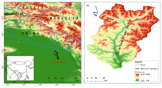
Figure 1.
(a) The secondary diagram shows the location of the study area (purple rectangular box) in China. The main diagram displays the location of the Irtysh river and the Altay mountain; (b) the elevation and drainage distribution of the study area. The elevation data is Space Shuttle Radar Terrain Mission (SRTM) provided by Geospatial Data Cloud site, Computer Network Information Center, Chinese Academy of Sciences. (http://www.gscloud.cn).
The Caiertes river basin (47–48N, 89–90E) is located in the southern slope of the Altay mountain in China. It is in the northeast-southwest direction and belongs to the northwest arid region of China. The elevation is 1150–3856 m (Figure 1b); it is high in the northeast and low in the southwest. Snow melt begins in early march and ends in early August in this basin. The westerly circulation in summer brings sufficient moisture to the Atlantic Ocean and forms abundant precipitation [28]. Due to the blocking of Siberian high pressure in winter [29,30], it is difficult for the water vapor transported by the westerly wind to reach the study area, and the precipitation is mainly affected by the cold air in Siberia and the air flow in the Arctic Ocean [30]. During the study period, water vapor in the study area originated from the northwest direction.
2.2. Remote Sensing Data
In this paper, Landsat 8 and Sentinel-2 were used to obtain the snow cover variations in time and space. Landsat 8 is the 8th satellite to be launched by the National Aeronautics and Space Administration (NASA) on February 11, 2013, carrying Operational Land Imager (OLI) and Thermal Infrared sensors (TIRS) [31,32]. Among them, OLI sensor covers 9 bands, the swath is 185 × 185 km, the revisit interval is 16 days, and the spatial resolution is 15–30m. In this study, a total of 10 images covering 10 days of Landsat8 OLI L1T (Level 1 Terrain-corrected) were downloaded from the USGS website (http://www.usgs.gov/). Among these 10 images, three images are completely covered by cloud and were excluded in this study. Sentinel-2 includes two high-resolution multispectral imaging satellites, Sentinel-2a (S2A) and Sentinel-2b (S2B), both of which carry a Multi-Spectral Imager (MSI) with 13 bands. The two satellites were launched on June 23, 2015 and March 07, 2017 respectively. The revisit interval of one satellite is 10 days, the two satellites complement each other, and the revisit interval is 5 days when two satellites are available. The spatial resolution is 30–60m, and the swath is 290km [33]. 284 scenes covering 71 days of Sentinel-2 MSI L1C (Level-1C) multispectral data are used in this study, which were downloaded from the ESA website (https://scihub.copernicus.eu/). A total of 27 days of these Sentinel-2 data are completely obscured by the cloud and 176 scenes covering 44 days were used subsequently for snow mapping. Two days of Sentinel-2 data and Landsat 8 OLI data were duplicated, so a total of 49 days of data sources could be used to obtain snow cover information during the study period. The spectral information used for image preprocessing and snow and cloud recognition in the two data sources is shown in Table 1. Band3(30m) and Band6(30m) of Landsat 8 OLI, and Band3(10m) and Band11(20m) of Sentinel-2 are used for snow mapping, respectively.

Table 1.
Partial band information of Landsat 8 OLI and Sentinel-2 MSI used in the study.
Preprocessing of Landsat-8 OLI and Sentinel-2 data was performed before snow and cloud mapping. The resolution of Landsat-8 OLI images was improved to 15 m by applying Gram-Schmidt Pan Sharpening in ENVI. Sen2cor tool was applied to L1C level data of Sentinel-2 for atmospheric correction to obtain Bottom-of-Atmosphere corrected reflectance of Sentinel-2 for snow mapping. LIC level data of Sentinel-2 was also used for cloud mapping in Section 3.3.2.
MODIS data was also used in this study to compare with Sentinel-2 and Landsat 8. The snow cover fraction of MODIS is from MOD10A1 product, which is available from the National Snow and Ice Data Center (NSIDC) Distributed Active Archive Center (DAAC).
2.3. Air Temperature Data
The air temperature used in the reconstruction model was from the Global Land Data Assimilation System (GLDAS) data. The data was developed by the National Aeronautics and Space Administration (NASA) the Goddard Earth Sciences Data and Information Services Center (GES DISC) [34], with a temporal resolution of 1 day. The spatial resolution could reach a maximum of 1/4 in the study area, which cannot truly reflect the air temperature variation characteristics caused by elevation change in a small watershed. Therefore, the digital elevation model of SRTM with a finer resolution of 1/10 was used to downscale the GLDAS air temperature in Figure 2. The absolute vertical error of SRTM DEM was less than 16 m [35]. Before elevation correction, SRTM elevation data after splicing and clipping were resampled and Gaussian-filtered to 1/10, and the original resolution of 1/4 of GLDAS air temperature data was then increased to 1/10 through the Gaussian filter. According to a certain lapse rate of air temperature, elevation correction of the filtered GLDAS's air temperature data was carried out to obtain the final air temperature with a resolution of 1/10.
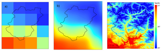
Figure 2.
GLDAS air temperature data and its processing results on April 1, 2018, including (a) 1/4 GLDAS air temperature, (b) 1/10 air temperature after the Gaussian filter, and (c) 1/10 air temperature after elevation correction.
In the Snowmelt-Runoff Model (SRM) or other air temperature elevation corrections, the air temperature lapse rate is usually set to a fixed value of −6.5 C/km [12,36]. However, in fact, the air temperature lapse rate changes with the change of season. Linear fitting of original GLDAS air temperature data and elevation for each day was performed in this study to calculate the optimized lapse rate k. When the determination coefficient R2 was greater than or equal to 0.8, the optimized lapse rate k was used further in air temperature downscaling; when the determination coefficient R2 was smaller than 0.8, the effective optimized lapse rate of adjacent time was used. In Figure 3, we can see that the rate before April is greater than −6.5 C/km, and that after April, it is almost less than −6.5 C/km, and the determination coefficient is mostly larger than 0.8. Section 5.2 describes the influence of dynamic estimation of the air temperature lapse rate on the maximum SWE accumulation in detail.
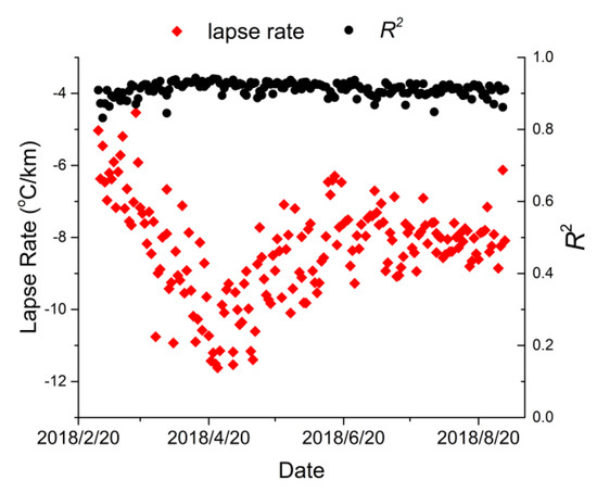
Figure 3.
The air temperature lapse rate after linear fitting in different seasons. The red points represent the air temperature lapse rate after linear fitting at a certain day, and the black points represent the determination coefficient, which is between 0 and 1.
2.4. Radiation Data
The net radiation index is the difference between the total incident energy of sunlight (the sum energy of long waves and short waves) and the total reflected energy from the ground, that is, downward radiation minus upward radiation. In this study, the net long-wave radiation is also from GLDAS with the temporal resolution of 1 day and the spatial resolution of 1/4. Studies on the spatial scale of the snow process have shown that the solar and thermal radiation inputs are biased at a resolution greater than 1/4, while the 1/10 grid of the energy flux produces results equivalent to 30 m and sufficient for the prediction of snowmelt runoff [37]. Therefore, we downscaled the resolution of the net long-wave radiation from GLDAS to 1/10, which requires setting a Gaussian filter with a size of 401 × 401 centering on the pixel with a resolution of 1/10, that is, the net long-wave radiation values of each pixel and other pixels within the neighborhood of 20 km are weight-averaged to obtain the pixel’s downscaled radiation values.
Considering the influence of mountain topography on solar radiation and the accuracy of shortwave radiation, we used Himawari-8 to calculate the hourly Shortwave Downward Radiation (SWDR) with a 90 m resolution after terrain correction. Himawari-8 estimates SWDR at a 10-min scale, and its high temporal resolution makes it more sensitive to cloud-radiation interactions and variations in surface radiation over a short period of time. First, the components of solar direct and diffuse radiation were derived from the 10-min Himawari-8 data [38], then a shortwave topographic radiation model (SWTRM) was applied [39]. Combined with MOD10A1 and MYD10A1 albedo product of MODIS, the upward radiation energy of solar radiation was calculated to obtain the net radiation index of short-wave radiation. In Section 5.3, the maximum SWE accumulation calculated by using net short-wave radiation from GLDAS, and Himawari-8/MODIS with terrain correction are compared.
3. Methodology
3.1. The SWE Reconstruction Model
Previous studies have shown that the reconstruction method can be used to estimate SWE at multiple spatial scales in complex terrain areas (mountain areas, river basins, etc.) [40,41]. Rittger et al. verified the reconstructed SWE with snow cover survey data and showed that the model could accurately estimate SWE values in different wet and dry years in different terrain environments [12]. It was also found that the model was very comparable to the measurement results of the NASA Airborne Snow Observatory (ASO) by measuring the snow cover area and improving the SRM model [2].
The purpose of the reconstruction is to calculate the maximum snow water equivalent for the whole season. The core idea is to carry out an inverse time series accumulation of the daily snowmelt amount from the time of complete snowmelt to the time of the beginning of snowmelt [12]:
In Equation (1), is the equivalent of snow water at the beginning of melting and the maximum value of a pixel at all time points. It serves as the total solid precipitation during the accumulation period and stable period of the snow season, excluding water loss such as evapotranspiration and soil infiltration. is the snow water equivalent on the Nth day after the maximum SWE occurs. The reverse calculation starts from , taking one day as the time step, Mj is the snowmelt amount on the day j, and is the snow water equivalent on the day n + 1. If n refers to the number of days between the date of the maximum SWE and complete snow melt, then and . Generally, drier years have an earlier maximum SWE, while wetter years have a later SWE. Considering the actual situation of the region and the selection time of remote sensing images, March 2nd is taken as the peak of SWE in the snow season of the research area from 2017 to 2018.
3.2. The Restricted Degree-Day Model
In the simple degree-day snowmelt model [23,42], the daily snowmelt amount of each hydrological response unit (HRU, in pixels) is only related to air temperature:
In Equation (2), (mm/day) is the ablation amount of one pixel on day j in the inverse time series, and the depth of snowmelt water is used to represent the amount of snowmelt. (mm/(day C)) is the degree-day factor; refers to the temperature that snow melt needs, which is generally considered to be the temperature of ice water mixture under standard atmospheric pressure, namely 0 C; and represents the average daily air temperature and generally means the average of the maximum and minimum daily air temperature values [36]. When is less than or equal to , the snowmelt amount is 0. When is greater than , air temperature values are converted into snowmelt by the degree-day factor.
Considering that the amount of snowmelt is related to the energy balance of the snow surface, in addition to the temperature, we added the daily net radiation value into the daily snowmelt model [43] and the restricted degree-day coefficient was used. The amount of ablation in each HRU in the restricted degree-day snowmelt model depends on the contribution of two parts: one is the air temperature value multiplied by the restricted degree-day factor (), and the other is the ablation amount proportional to the net radiation index (W m−2).
In Equation (3), ((mm day−1)/(W m−2)) is similar to in Equation (2), and is a physical constant used to convert energy into the water depth, and the value is usually set at 0.26 [12] (mm/(day C)) is a restricted degree-day factor, and the value is 1.5 [40,43], which is not equal to in Equation (2), but both values are multiplied by the air temperature value .
In Equations (2) and (3), the two snow melt models calculate the snow melt amount when the snow cover of each pixel is 100%. In practical conditions, pure snow pixels do not always exist. Therefore, we multiplied the snow melt amount of a single pixel by the snow cover fraction of the pixel (0%–100%), as the daily snow melt amount on the pixel scale:
The maximum SWE of the whole snow season was then calculated by substituting the daily snow melt amount obtained from Equation (4) into Equation (1). Compared with the simple calculation method of the degree-day snowmelt water model in Equation (2), net radiation is introduced in Equation (3) to better describe the energy balance of snow. The heterogeneity of snow cover in space and the characteristics of snow cover in the watershed are considered in Equation (4) in a more objective and detailed way, thus snow melt can be estimated with a higher accuracy.
3.3. Snow Cover
3.3.1. Snow Detection
There are many methods for the snow identification of remote sensing images, including the snow index method [44,45], the MODIS Snow Covered Area and Grain Size (MODSCAG) algorithm [46], machine-learning-based decision tree classification [33], etc. These methods have different adaptabilities to remote sensing images for different sources and different regions, among which the SNOWMAP algorithm based on the snow index method is the most widely used. The SNOWMAP algorithm was developed and tested using Landsat TM data [45], prior to the launch of MODIS [47]. According to the results of manual visual interpretation, the algorithm is also applicable to the Sentinel-2 satellite image in the Caiertes river basin. Its physical basis is as follows: both snow cover and cloud have a high reflectance in the visible band, while snow cover has strong absorption characteristics in the SWIR band, but most clouds still have a high reflectance in the SWIR band. With such differences of spectral characteristics, the snow pixel can be easily identified from the cloud by setting a threshold for the Normalized Difference Snow Index (NDSI). The calculation of NDSI is
In Equation (5), Green is the reflectance of snow in the green band and SWIR is the reflectance of snow in the SWIR band. For Sentinel-2, band3 (Green, 0.56 ) and band11 (SWIR1, 0.61 ) are used, and for Landsat 8 OLI data, band3 (Green, 0.525–0.600 ) and band6 (SWIR1, 1.560–1.651 ) are used. The study of snow cover in the Sierra Nevada in California, USA [44] and in the Indian Himalayan basin [48] has shown that NDSI 0.4 can be used as a criterion for identifying snow in Landsat 7 images. Negi et al. also found that this criterion could ignore the impact of slope and aspect changes caused by topography on the threshold [48]. In addition, Kulkarni et al. found that the threshold value of NDSI would not be affected by mountain shadow [49]. Based on these studies, the NDSI threshold of the SNOWMAP algorithm was set as 0.4, and when NDSI 0.4, the pixel was defined as snow. However, due to different observation times and multiple sources of images, NDSI thresholds could not be fixed in this study. In the process of snow identification, different thresholds were set according to different remote sensing images and sensing time. The thresholds of Sentinel-2 were between 0.35 and 0.45, and those of Landsat 8 were between 0.3 and 0.4.
Snow and water also have similar spectral characteristics in the visible and SWIR bands. In order to further identify snow from water, we used the feature of the strong absorption of water in the NIR band, while the absorption of snow is weaker than that of water [47]. Therefore, another discriminating criterion of snow recognition was added into SNOWMAP:
In Equation (6), NIR refers to the reflectance of the near-infrared band, corresponding to band8 of Sentinel-2 (0.842 ) and band5 of Landsat 8 OLI (0.845–0.885 ). When NDSI 0.4 and NIR 0.11, the pixel is recognized as snow cover.
In addition, when the vegetation coverage is relatively high, the signal of snow cover observation will be attenuated, so some NDSI pixels lower than 0.4 can also be considered as snow cover. In this study, vegetation coverage products [42] were adopted to identify snow pixels affected by vegetation coverage. When the vegetation coverage is more than 40% and the conditions of NDSI 0.1 and NIR 0.11, the pixel is also considered as snow.
3.3.2. Cloud Detection and Interpolation
In snow cover extraction, the cloud cover and cloud discrimination algorithm are the main factors affecting the data continuity and accuracy. Before the snow cover classification based on NDSI and NDVI is carried out, an important step is to carry out preprocessing for the cloud removal of images. Due to the long period of this study, significant differences in climate and environment, and diverse cloud forms, we found that only one cloud detection algorithm could not be used for all images. Therefore, according to their morphology and spectral characteristics, clouds were classified into cirrus clouds, dense clouds, and ice clouds. Based on the threshold value of existing studies, Sentinel-2 was taken as an example to conduct an adaptive analysis for this research area and a new combined identification algorithm is proposed.
Cirrus clouds are high-altitude clouds, for which the altitude is typically between 4500 and 10,000 m, and can be classified as ice clouds. They are composed of fine ice crystals which are relatively sparse in the upper air, so the clouds are relatively thin and they have good light transmission. This type of cloud is too thin, transparent, or translucent to be easily recognized. Hollstein et al. used a machine learning algorithm [50] to effectively identify cirrus clouds [33]. By training a given data set, it returns an optimized decision tree algorithm with a given depth. The purpose of this method is to find an optimal classification method without additional parameters. When the given depth is set to four layers, more than a 91% correct classification accuracy can be achieved. In this study, we found that this algorithm is very suitable for cirrus removal in the research area of the Caiertes river basin. The identification index used is
In Equations (7) and (8), B, R, and S refer to the reflectance, ratio, and difference of the corresponding band of images, respectively. For example, B3 represents the reflectance of band3 of Sentinel-2 MSI, R(2,10) represents the ratio of band2 to band10, and S(11,10) represents the difference between band11 and band10. When Equations (7) and (8) are applied simultaneously, the pixel can be considered as cirrus.
Dense cloud, also known as opaque cloud, is identified by the cloud mask algorithm of the Sentinel-2 LIC product [51]. Dense clouds and snow have a high reflectance in the blue region (B2, 0.49 ), but snow has a much lower reflectance than dense clouds in the SWIR band (B11 and B12, 1.61 and 2.19 ), so they can be separated by setting thresholds in the SWIR band. Additionally, some ice clouds show ice crystals on the cloud top due to their high altitude, resulting in low reflectance, similar to snow in SWIR band B11 and B12, which is difficult to distinguish. Therefore, a threshold of SWIR band B10 (1.375 ) is needed to identify ice clouds with a higher altitude. In this step of ice cloud recognition, cirrus clouds at the same altitude will not be recognized, as they are transparent in the blue band B2 [51].
After obtaining the snow and cloud cover data during the study period, we interpolated the cloud pixels and pixels without effective data according to the continuous characteristics of snow cover in time and space. The linear interpolation method was used in time interpolation, which is robust and efficient. A three-dimensional Gaussian filter was used in spatial interpolation to make the snow cover more continuous in time and space [52]. By performing interpolation to the binary snow and cloud mapping results, we can get the daily fraction snow cover (). Figure 4 shows the interpolation results in which the data loss caused by cloud cover is filled. The characteristics of snow cover changing with topography can also be identified from Figure 4. The interpolation method is also applicable to MOD10A1 snow cover products.
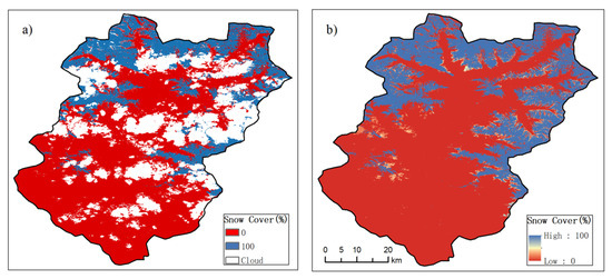
Figure 4.
A comparison of before (a) and after (b) the spatiotemporal interpolation on June 8, 2018. Blue represents the area with complete snow cover ( = 100%), and red represents the area without snow ( = 0). White in (a) represents the area covered by cloud (i.e., the area to be interpolated), while the area mediated between blue and red in (b) is the area covered by incomplete snow ( is between 0 and 100%).
4. Results
4.1. Snow Cover Characteristics in a Mountainous Area
4.1.1. Temporal Variation
Time series snow cover fractions of every 300 m elevation band of the whole basin are shown in Figure 5. It shows that the snow cover in the whole basin began to melt on March 2, 2018, and nearly disappeared in late July. Snow cover was close to 100% on March 2 and almost zero in late July. The snow cover gradually decreases with time, but there will also be a sudden increase of snow cover, which is because of the phenomenon of new snow after the beginning of the ablation period. There are differences in the starting and disappearing time of snow cover at different elevations: the higher the altitude, the later the melting time, and the later the disappearing time. In the early stage of snowmelt (March), the snow at a low altitude (less than 2200 m) begins to melt first; the higher the altitude, the slower the snow area shrinks. In the middle period of snowmelt (April and May), the air temperature gradually increases, and the shrinking rate of snow cover slightly accelerates. In the later period of snowmelt (June and July), the low-altitude snow cover completely disappears, while the high-altitude snow cover (over 2800 m) begins to disappear, and ends in early August. The ablation process of each elevation zone also has some similar characteristics: the area shrinkage rate is basically similar, and the ablation takes about 2 months. The reasons for this phenomenon will be explained in Section 4.2.1.
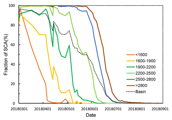
Figure 5.
Daily variation of snow cover fraction () in the whole watershed and its elevation zones. The black dotted line represents the time series change of snow cover in the whole basin, while the colored solid line represents the change of each elevation zone.
4.1.2. Spatial Variation
In order to show snow cover variation spatially, distribution maps of snow cover on the first day of each month in the ablation period are shown in Figure 6. The accumulated peak of snow cover is in early March, when almost the whole basin is covered with snow. However, some areas were affected by human activities, air temperature rising, radiation enhancement, and other factors at the valley bottom, resulting in snow melt and incomplete snow cover. From March to June, the snow cover gradually decreases, and the snow shrinks from the valley bottom to the peak. The time of the beginning and completion of melting of the low altitude is earlier than that of the high altitude, which is consistent with the conclusion in Section 4.1.1. Compared with Figure 5, it is found that the snow melt is basically completed in early July, and then, only a small part of the snow above the altitude of 2500 m exists. In early August, the snow cover is almost 0.
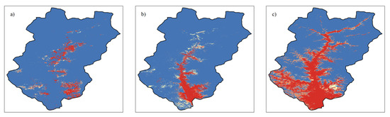
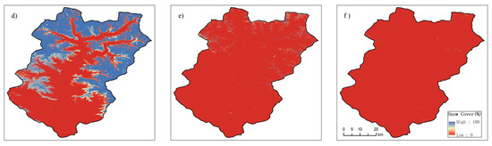
Figure 6.
Spatial variation characteristics of snow cover (). (a–f) represent snow cover on the first day of March–August respectively; blue represents the snow covered area; red represents the no snow cover area; and other colors represent the areas with snow cover, but not complete cover, the snow cover of which is between 0 and 100%. Among them, yellow represents the area with snow cover of 0.5, and light blue represents the area with almost full snow cover.
4.2. The Reconstructed SWE
4.2.1. Temporal Variation
We also divided the SWE according to an elevation band of 300 m, and then recorded statistics of its change characteristics with time. Figure 7 shows that the mean maximum SWE accumulation during the initial snowmelt period of the whole basin is 377.83mm. The SWE decreases to 0 gradually with time and lasts for a total time span of 5 months. The mean maximum SWE accumulation of each elevation band increases with the increase of altitude and also decreases with time in the ablation period. As the altitude increases, it takes longer for SWE to decrease to 0. Different from the retreat rate of snow cover in Section 4.1.1, the higher the altitude is, the faster the snow ablation rate will be. This is because the ablation rate is related to air temperature and the net radiation at the time of ablation, while the retreat of the snow cover area is not only related to the ablation rate, but also the SWE. Even though the melting rate in high-altitude areas accelerates in the later stage of snowmelt, the snow area shrinkage rate is close to that in low-altitude areas as the SWE at a high altitude is much larger than that in low-altitude areas. This also explains why there are different maximum SWE accumulation values at the beginning of ablation for different elevation bands, but the ablation process for all elevation bands takes about 2 months.
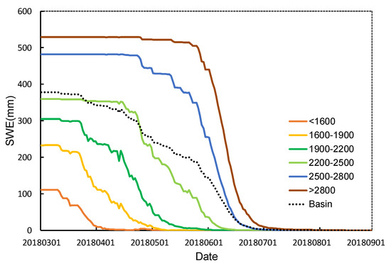
Figure 7.
Daily variation of the snow water equivalent (SWE) in the whole basin and at different elevation bands. The range of elevation zone represented by the legend is consistent with Figure 5. The black dotted line represents the temporal change of SWE of the whole basin, and the solid colored line represents the change of SWE at each elevation band, respectively.
4.2.2. Spatial Variation
Figure 8 shows the distribution of maximum SWE accumulation in the study area. SWE gradually increased from valley to peak, which is consistent with the conclusion in Section 4.2.1. In Figure 11a, the scatter density map of maximum SWE accumulation and elevation is shown. We found that the maximum SWE accumulation increases with elevation in the area which has an elevation below 2800 m. However, there was a turning point at 2800 m. SWE above 2800 m did not increase completely with elevation, but decreased more significantly. This conclusion is consistent with the results of Grünewald and Rittger et al. [12,53], which are caused by the topographic effect [12].
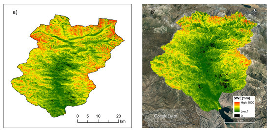
Figure 8.
Two-dimensional (a) and three-dimensional (b) spatial distribution of the maximum SWE at the initial stage of snowmelt.
The distribution of maximum SWE accumulation calculated by Sentinel-2/Landsat snow cover at a local scale is shown in Figure 9b,e. The application of high-resolution remote sensing data in the SWE reconstruction offers a detailed description of the local SWE spatial distribution over mountain terrain. However, the distribution of maximum SWE accumulation calculated by MOD10A1 snow cover product shown in Figure 9c,f hardly reflects the distribution characteristics of snow affected by local topography. Even in some local areas, as shown in Figure 9c, the snow cover area is underestimated due to the low spatial resolution of MODIS image, leading to inaccurate SWE calculation.
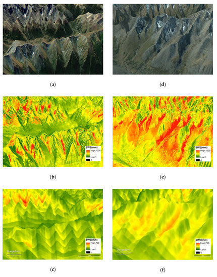
Figure 9.
Spatial distribution of the local maximum SWE accumulation calculated by Sentinel-2/Landsat (b and e) and MOD10A1 (c and f) snow cover at the early stage of snowmelt. (a) and (d) represent the distribution of local terrain in Google Earth, and height is exaggerated in Google Earth with a coefficient of 3.0. The regions in these figures are respectively located at (a–c) 47.702682N,89.950935E and (d–f) 47.784629N, 89.660171E.
Figure 8 shows that the maximum SWE accumulation occurs in areas with a high altitude (above 2800 m), where the slope, aspect, and other topographic characteristics are good for the storage of snow. In Figure 9, large SWE accumulation areas are caused by local topography, which means that snow can be stored in such local basins, as well as blowing snow. On the other hand, it is difficult for snow to be stored in areas with a steep slope. For example, the high SWE accumulation area such as the valley in Figure 9a–c has the characteristics of low-lying flat terrain, which is conducive to the accumulation of snow, while the slope of the yellow region is larger, which is not conducive to the retention of snow. In Figure 9d–f, the high SWE area is located under steep slopes, which is probably caused by the sliding of snow from the upper slopes. However, there is another possibility: the red area is located on the northern slope of the mountain, and the SWE of the northern slope is larger than that of the southern slope due to the influence of the water vapor source [30] and wind direction.
5. Discussion
5.1. Snow Cover of Sentinel-2/Landsat and MODIS
The time series snow cover fraction and SWE of the whole basin derived from Sentinel-2/Landsat and MOD10A1 are shown in Figure 10. As shown in Figure 10, the snow cover fraction from MOD10A1 is significantly lower than that from Sentinel-2/Landsat. For the whole snowmelt season, the snow cover fraction is underestimated by 37.64% compared to snow cover fraction from Sentinel-2/Landsat. The maximum snow cover on March 2 was underestimated by 32.28%; The underestimated error of snow cover from March to May did not change significantly, which is about 30%. Figure 10b also shows that the SWE reconstructed by MOD10A1 snow cover area is lower than the SWE calculated by the snow cover parameter obtained in this study, and the SWE is underestimated by an average of 58.72% in the whole snowmelt season. From March to May, the underestimated error of SWE was close to that of 31.31% on average.
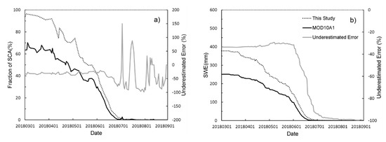
Figure 10.
Time series comparison of snow cover (a) and reconstructed SWE (b) from different image sources. The dotted line represents the results obtained using Landsat 8 and Sentinel-2 data in this study, and the solid line represents the results obtained from the MOD10A1 snow cover day products.
5.2. Air Temperature
The maximum SWE accumulation was calculated by using an optimized air temperature lapse rate and fixed lapse rate. The relationship between elevation and maximum SWE accumulation calculated by these two methods is shown in Figure 11a,b, respectively. For both results, the maximum SWE accumulation increases with increasing elevation under 2800 m, and the maximum SWE accumulation then starts to decrease with increasing elevation beyond 2800 m. The difference of the results by using the optimized air temperature lapse rate or fixed lapse rate lies in that the maximum SWE accumulation of the optimized lapse rate method is smaller than that of the fixed lapse rate method for elevations larger than 2300 m (Figure 11c). This is because the optimized air temperature lapse rate after ablation season fitting is lower than the fixed lapse rate for most of the time period. Therefore, the air temperature above average elevation calculated by using the optimized lapse rate is lower than that calculated by using the fixed lapse rate, while the air temperature below average elevation calculated by using the optimized lapse rate is higher than that calculated by using the fixed lapse rate. In addition, the snow melt time in low elevation areas is short and is not sensitive to the lapse rate, and the reconstructed SWE in the high-elevation area is more affected by the lapse rate used in air temperature downscaling.
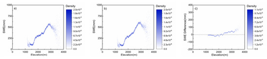
Figure 11.
(a,b) The relationship between maximum SWE accumulation and elevation in mountainous areas. (a) represents the calculated SWE by using optimized air temperature lapse rate, and (b) represents the calculated SWE using a fixed lapse rate of −6.5 C/km. (c)The scatter plot of the SWE difference between the SWE calculated by using optimized air temperature lapse rate and a fixed lapse rate of −6.5 C/km.
5.3. Solar Radiation
Figure 12a,b shows the relationship between aspect and maximum SWE accumulation calculated by the Himiwari-8 solar radiation with terrain correction and the GLDAS short-wave radiation without terrain correction. Maximum SWE accumulation obtained from the two kinds of solar radiation data has the same trend with respect to aspect. The SWE in the north slope (0–45 and 315–356) is larger than that in the south slope (135–225), and the SWE in the east and west slope is close to each other. However, the SWE calculated with terrain correction is smaller than that without terrain correction in all directions in different levels. Figure 12c shows that the difference between the two results on the north slope is greater than that on the south slope. In addition, we also calculated the RMSE of these two kinds of radiation data on the north and south slope respectively to evaluate the difference between the two types of radiation data on the north and south slope. The RMSE of south slope and north slope is 182.67 and 269.01 respectively. The SWE values of the south slope are close to each other, while the value deviation of the north slope is large. Therefore, it can be concluded that the difference of SWE between north and south slope after terrain correction is smaller than that without correction. The solar radiation corrected by topography is weaker on the north slope than on the south slope due to the influence of mountain shadows. Therefore, not only natural factors such as topography, but also the calculation of solar radiation also affects the spatial distribution difference of maximum SWE accumulation on aspect.
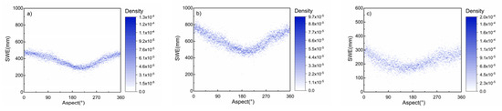
Figure 12.
(a,b) The relationship between the maximum SWE accumulation and aspect in mountainous areas at the beginning of snowmelt. (a) represents the calculated SWE after terrain correction, and (b) represents the SWE without terrain correction. (c) The scatter plot of SWE difference between the topographic corrected SWE and the non-corrected SWE.
5.4. Error Analysis
Wind plays a key role in sublimation [54], but the wind speed in the Altay mountains is small, which is negligible compared with snow melt caused by air temperature and radiation energy. The errors of the reconstructed model mainly come from the errors of the input parameters in the restricted degree-day model and errors in the model itself.
Snow cover is one of the most important parameters affecting the accuracy of SWE reconstruction. Section 5.1 proved MOD10A1 snow products to be underestimated, due to the serious omission error caused by the resolution of MODIS 500 m in areas with mountain shadows and the edge of snow cover [55]. In this study, since the cloud may not have separated from the snow during snow recognition, it is possible to overestimate snow recognition from Landsat 8 and Sentinel-2 images.
In this study, a revisit time of about 3–4 days can be achieved by combing Sentinel-2 and Landsat images, and this makes the retrieval of snow cover variation in fine spatial and temporal resolution possible. In order to obtain the snow cover under cloud, linear interpolation in time and Gaussian filter in space are performed. However, when a certain pixel is covered by cloud for a long period of time and in the meanwhile the snow cover changes significantly in this time period, linear interpolation is not accurate. Fortunately, this situation is rare. When more satellite images with tens of meters resolution are included, such as GF-1 and GF-6 satellites, this problem can be effectively solved.
The degree-day factor in the restricted degree-day model depends on the air temperature data, which can only be calculated with the reanalysis data. The seasonal variation of degree-day factors is large, which requires a large amount of actual data correction. In addition, Brubaker et al. found that, in addition to air temperature, when using long and shortwave net radiation energy, the performance of the model was less dependent on the restricted degree-day factor and had greater universality. The model could be extended to areas lacking actual measurement experience [43]. Marks and Dozier confirmed that solar radiation in the Sierra Nevada, California, USA, contributes more to snow melt than air temperature parameters, but air temperature also plays a role in the studied region [56]. In Section 5.2, the SWE difference estimated before and after fitting of the linear air temperature lapse rate reaches 38.26mm to the maximum extent at the elevation (2800 m) of the SWE maximum, accounting for about 7.01% of the maximum estimated SWE in the same elevation.
According to Mahat et al. [57] and Brubaker et al. [43], the conversion factor of the radiation parameter represents the coefficient of conversion of any form of energy (W/m2) into the amount of snow melt (mm/day) when the snow temperature is equal to 0 C, which is fixed in theory. In Section 5.3, the SWE calculated by GLDAS is larger than that calculated by SWDR after terrain correction, so the net short-wave radiation data of GLDAS is larger than the net short-wave radiation calculated by SWDR and MOD10A1 albedo products. This may be due to the high value of GLDAS, or the low value of SWDR and the high value of albedo. GLDAS long-wave radiation data without terrain correction will also affect the estimation of maximum SWE accumulation to some extent.
In mountainous areas with high precipitation uncertainty, the accumulation of daily snowmelt can only reflect the change of new snow area in the snowless area, but not in the snow-covered area. The new snow will be considered as the original snowpack, and the estimated value of the maximum SWE accumulation will be overestimated. However, compared with other measurement methods, estimation of the reconstruction method is more in line with the actual situation [58].
The tree cover fraction is very low in the study area, so the influence of tree attenuation on radiation is not considered in this study. In further work, tree attenuation of radiation should be considered by calculating radiation under the tree canopy.
6. Conclusions and Outlook
In this study, the seasonal maximum SWE accumulation in a mountainous area has been reconstructed using multi-source remote sensing images with resolutions of tens of meters. The combination of Landsat 8 and Sentinel-2 satellite images improved the accuracy of snow cover parameters of the reconstructed model, which greatly improved the retrieval accuracy and spatial resolution of the SWE in mountainous areas. In this case, complex pixel unmixing efforts can be avoided when estimating the fractional snow cover. Snow in the Caiertes river basin disappeared in late July for five months. The melting date and vanishing date of snow at different altitudes are different, but they all last about 2 months. In the spatial distribution of snow cover, the melting and disappearing time of snow is getting earlier and earlier from the valley to the top of the mountain. The area shrinking rate of each elevation zone is basically similar. However, the higher the altitude, the faster the snow melts. The average maximum SWE accumulation of the whole basin at the beginning of snowmelt is 377.83 mm. In the early stage of snowmelt, the maximum SWE accumulation increases with elevation, but in the area above 2800 m, the SWE decreases with elevation. Compared with MOD10A1 snow cover products, the reconstruction technology can describe the maximum SWE accumulation distribution characteristics of local snow cover in mountainous areas with a higher accuracy by using high-resolution remote sensing images to extract the snow cover area. In addition to regional elevation, the slope, aspect, and other topographic features all affect the accumulation and storage of snow. The errors of the reconstructed model are mainly derived from air temperature and radiation, as well as the estimated values of the snow cover area. Therefore, the accuracy of each parameter of the reconstructed model is very important to the accuracy of the results. In future research, air temperature and radiation data with higher accuracy are expected to improve the accuracy of SWE. Other freely available remote sensing data with a tens of meters spatial resolution (such as the Chinese Gaofen-1 and Gaofen-6 satellite data) could also be added to the snow cover mapping scheme, which would improve the temporal resolution of snow mapping. Furthermore, to validate the absolute value of reconstructed maximum SWE results, snow depth and SWE ground stations are needed on the mountains in this basin in the future.
Author Contributions
Conceptualization, C.X.; Data curation, M.L., J.P. and T.W.; Formal analysis, M.L.; Funding acquisition, J.S.; Investigation, M.L. and C.X.; Methodology, C.X. and J.P.; Project administration, C.X.; Software, M.L.; Supervision, C.X., J.S. and N.W.; Visualization, M.L.; Writing—original draft, M.L.; Writing—review and editing, C.X. and N.W. All authors have read and agree to the published version of the manuscript.
Funding
This research was funded by the Strategic Priority Research Program of the Chinese Academy of Sciences (Grant No. XDA20100300): Study on water resources in Asia water tower area; the Strategic Priority Research Program of the Chinese Academy of Sciences (Grant No. XDA19070302): Study on the change of tripolar ice pool and the runoff of large rivers in the Arctic Circle; Science and Technology Basic Resources Investigation Program of China (Grant No.2017FY100501): Survey of basic elements of snow in China.
Conflicts of Interest
The authors declare no conflict of interest.
References
- Barnett, T.P.; Adam, J.C.; Lettenmaier, D.P. Potential impacts of a warming climate on water availability in snow-dominated regions. Nature 2005, 438, 303. [Google Scholar] [CrossRef] [PubMed]
- Bair, E.H.; Rittger, K.; Davis, R.E.; Painter, T.H.; Dozier, J. Validating reconstruction of snow water equivalent in California's Sierra Nevada using measurements from the NASAAirborne Snow Observatory. Water Resour. Res. 2016, 52, 8437–8460. [Google Scholar] [CrossRef]
- Shen, Y.P.; Su, H.C.; Wang, G.Y.; Mao, W.M.; Wang, D.S.; Han, P.; Wang, N.L.; Li, Z.Q. The responses of glaciers and snow cover to climate change in Xinjiang (Ⅰ): Hydrological effect. J. Glaciol. Geocryol. 2013, 3, 513–527. [Google Scholar]
- Pan, J.M.; Jiang, L.M.; Zhang, L.X. Snowmelt estimation of Iii River basin based on physically-based snow process model. In Symposium on Application of Space Information Technology in Water Conservancy Field by China Water Conservancy Society; MDPI: Beijing, China, 2010. [Google Scholar]
- Shen, Y.P.; Su, H.C.; Wang, G.Y.; Mao, W.M.; Wang, D.S.; Han, P.; Wang, N.L.; Li, Z.Q. The responses of glaciers and snow cover to climate change in Xinjiang (Ⅱ): Hazards Effects. J. Glaciol. Geocryol. 2013, 35, 1355–1370. [Google Scholar]
- Zhao, Q.D.; Liu, Z.H.; Fang, S.F.; Lu, Z.; Wang, Y.F.; Li, M. Improved Snowmelt Model Based on EOS/MODIS Remote Sensing Data. J. Arid Land 2007, 30, 915–920. [Google Scholar]
- Zhang, P.; Wang, J.; Liu, Y.; Li, Y. Application of SRM to Flood Forecast and Forwarning of Manasi River Basin in Spring. Remote Sens. Technol. Appl. 2009, 24, 456–461. [Google Scholar]
- Abudu, S.; Cui, C.; King, J.P.; Abudukadeer, K. Comparison of performance of statistical models in forecasting monthly streamflow of Kizil River, China. Water Sci. Eng. 2010, 3, 269–281. [Google Scholar]
- Shi, J.C.; Xiong, C.; Jiang, L.M. Review of snow water equivalent microwave remote sensing. Sci. China Ser. D Earth Sci. 2016, 59, 731–745. [Google Scholar] [CrossRef]
- Dozier, J.; Bair, E.H.; Davis, R.E. Estimating the spatial distribution of snow water equivalent in the world’s mountains. WIREs Water 2016, 3, 461–474. [Google Scholar] [CrossRef]
- Rice, R.; Bales, R.C.; Painter, T.H.; Dozier, J. Snow water equivalent along elevation gradients in the Merced and Tuolumne River basins of the Sierra Nevada. Water Resour. Res. 2011, 47. [Google Scholar] [CrossRef]
- Rittger, K.; Bair, E.H.; Kahl, A.; Dozier, J. Spatial estimates of snow water equivalent from reconstruction. Adv. Water Resour. 2016, 94, 345–363. [Google Scholar] [CrossRef]
- Fassnacht, S.R.; Dressler, K.A.; Bales, R.C. Snow water equivalent interpolation for the Colorado River Basin from snow telemetry (SNOTEL) data. Water Resour. Res. 2003, 39. [Google Scholar] [CrossRef]
- Mätzler, C. Applications of the interaction of microwaves with the natural snow cover. Remote Sens. Rev. 1987, 2, 259–387. [Google Scholar] [CrossRef]
- Chang, A.; Foster, J.L.; Hall, D.K. Nimbus-7 SMMR derived global snow cover parameters. Ann. Glaciol. 1987, 9, 39–44. [Google Scholar] [CrossRef]
- Kurvonen, L.; Hallikainen, M. Influence of land-cover category on brightness temperature of snow. IEEE Trans. Geosci. Remote 1997, 35, 367–377. [Google Scholar] [CrossRef]
- Wiesmann, A.; Mätzler, C.; Weise, T. Radiometric and structural measurements of snow samples. Radio Sci. 1998, 33, 273–389. [Google Scholar] [CrossRef]
- Sun, Z.W.; Shi, J.C.; Jiang, L.M.; Yang, H.; Zhang, L.X. Development of snow depth and snow water equivalent algorithm in Western China using passive microwave remote sensing data. Adv. Earth Sci. 2006, 21, 1363–1369. [Google Scholar]
- Che, T.; Li, X.; Jin, R.; Armstrong, R.; Zhang, T. Snow depth derived from passive microwave remote-sensing data in China. Ann. Glaciol. 2008, 49, 145–154. [Google Scholar] [CrossRef]
- Jiang, L.M.; Wang, P.; Zhang, L.X.; Yang, H.; Yang, J.T. Improvement of snow depth retrieval for FY3B-MWRI in China. Sci. China Ser. D Earth Sci. 2014, 57, 1278–1292. [Google Scholar] [CrossRef]
- Clow, D.W.; Nanus, L.; Verdin, K.L.; Schmidt, J. Evaluation of SNODAS snow depth and snow water equivalent estimates for the Colorado Rocky Mountains, USA. Hydrol. Process. 2012, 26, 2583–2591. [Google Scholar] [CrossRef]
- National Operational Hydrologic Remote Sensing Center Snow Data Assimilation System (SNODAS) Products at NSIDC: National Snow and Ice Data Center. Available online: https://nsidc.org/sites/nsidc.org/files/files/nsidc_special_report_11.pdf (accessed on 15 January 2020).
- Martinec, J.; Rango, A. Areal distribution of snow water equivalent evaluated by snow cover monitoring. Water Resour. Res. 1981, 17, 1480–1488. [Google Scholar] [CrossRef]
- Molotch, N.P.; Bales, R.C. Scaling snow observations from the point to the grid element: Implications for observation network design. Water Resour. Res. 2005, 41. [Google Scholar] [CrossRef]
- Lettenmaier, D.P.; Alsdorf, D.; Dozier, J.; Huffman, G.J.; Pan, M.; Wood, E.F. Inroads of remote sensing into hydrologic science during the WRR era. Water Resour. Res. 2015, 51, 7309–7342. [Google Scholar] [CrossRef]
- Bair, E.H.; Abreu Calfa, A.A.; Rittger, K.; Dozier, J. Using machine learning for real-time estimates of snow water equivalent in the watersheds of Afghanistan. Cryosphere 2018, 12, 1579–1594. [Google Scholar] [CrossRef]
- GDAL/OGR Contributors. GDAL/OGR Geospatial Data Abstraction Software Library. Open Source Geospatial Foundation. Available online: https://gdal.org (accessed on 17 January 2020).
- Zhang, Y.; Enomoto, H.; Ohata, T.; Kitabata, H.; Kadota, T.; Hirabayashi, Y. Glacier mass balance and its potential impacts in the Altai Mountains over the period 1990–2011. J. Hydrol. 2017, 553, 662–677. [Google Scholar] [CrossRef]
- Panagiotopoulos, F.; Shahgedanova, M.; Hannachi, A.; Stephenson, D.B. Observed trends and teleconnections of the Siberian high: A recently declining center of action. J. Climat. 2005, 18, 1411–1422. [Google Scholar] [CrossRef]
- Yao, X.J.; Liu, S.Y.; Guo, W.Q.; Huai, B.J.; Sun, M.P.; Xu, J.L. Glacier Change of Altay Mountain in China from 1960 to 2009—Based on the Second Glacier Inventory of China. Nat. Resour. 2012, 27, 1734–1745. [Google Scholar]
- Roy, D.P.; Wulder, M.A.; Loveland, T.R.; Woodcock, C.E.; Allen, R.G.; Anderson, M.C.; Helder, D.; Irons, J.R.; Johnson, D.M.; Kennedy, R.; et al. Landsat-8: Science and product vision for terrestrial global change research. Remote Sens. Environ. 2014, 145, 154–172. [Google Scholar] [CrossRef]
- Irons, J.R.; Dwyer, J.L.; Barsi, J.A. The next Landsat satellite: The Landsat data continuity mission. Remote Sens. Environ. 2012, 122, 11–21. [Google Scholar] [CrossRef]
- Hollstein, A.; Segl, K.; Guanter, L.; Brell, M.; Enesco, M. Ready-to-use methods for the detection of clouds, cirrus, snow, shadow, water and clear sky pixels in Sentinel-2 MSI images. Remote Sens.-Basel. 2016, 8, 666. [Google Scholar] [CrossRef]
- Rodell, M.; Houser, P.R.; Jambor, U.; Gottschalck, J.; Mitchell, K.; Meng, C.-J.; Arsenault, K.; Cosgrove, B.; Radakovich, J.; Bosilovich, M.; et al. The global land data assimilation system. Bull. Am. Meteorol. Soc. 2004, 85, 381–394. [Google Scholar] [CrossRef]
- Farr, T.G.; Rosen, P.A.; Caro, E.; Crippen, R.; Duren, R.; Hensley, S.; Kobrick, M.; Paller, M.; Rodriguez, E.; Roth, L. The shuttle radar topography mission. Rev. Geophys. 2007, 45. [Google Scholar] [CrossRef]
- Martinec, J.; Rango, A.; Major, E. The Snowmelt-Runoff Model (SRM) User’s Manual. 1983. Available online: https://ntrs.nasa.gov/search.jsp?R=19830015389 (accessed on 15 January 2020).
- Winstral, A.; Marks, D.; Gurney, R. Assessing the sensitivities of a distributed snow model to forcing data resolution. J. Hydrometeorol. 2014, 15, 1366–1383. [Google Scholar] [CrossRef]
- Yu, Y.; Wang, T.; Shi, J.; Zhou, W. A Lut-Based Method to Estimate Clear-Sky Instantaneous Land Surface Shortwave Downward Radiation and its Direct Component from Modis Data. In Proceedings of the IGARSS 2019–2019 IEEE International Geoscience and Remote Sensing Symposium, IEEE, Yokohama, Japan, 28 July–2 August 2019; pp. 1861–1864. [Google Scholar] [CrossRef]
- Wang, T.; Yan, G.; Mu, X.; Jiao, Z.; Chen, L.; Chu, Q. Toward operational shortwave radiation modeling and retrieval over rugged terrain. Remote Sens. Environ. 2018, 205, 419–433. [Google Scholar] [CrossRef]
- Molotch, N.P.; Margulis, S.A. Estimating the distribution of snow water equivalent using remotely sensed snow cover data and a spatially distributed snowmelt model: A multi-resolution, multi-sensor comparison. Adv. Water Resour. 2008, 31, 1503–1514. [Google Scholar] [CrossRef]
- Molotch, N.P. Reconstructing snow water equivalent in the Rio Grande headwaters using remotely sensed snow cover data and a spatially distributed snowmelt model. Hydrol. Process 2009, 23, 1076–1089. [Google Scholar] [CrossRef]
- Rango, A.; Martinec, J. REVISITING THE DEGREE-DAY METHOD FOR SNOWMELT COMPUTATIONS 1. J. Am. Water Resour. Assoc. 1995, 31, 657–669. [Google Scholar] [CrossRef]
- Brubaker, K.; Rango, A.; Kustas, W. Incorporating radiation inputs into the snowmelt runoff model. Hydrol. Process. 1996, 10, 1329–1343. [Google Scholar] [CrossRef]
- Dozier, J. Spectral signature of alpine snow cover from the Landsat Thematic Mapper. Remote Sens. Environ. 1989, 28, 9–22. [Google Scholar] [CrossRef]
- Chokmani, K.; Dever, K.; Bernier, M.; Gauthier, Y.; Paquet, L. Adaptation of the SNOWMAP algorithm for snow mapping over eastern Canada using Landsat-TM imagery. Hydrol. Sci. J. 2010, 55, 649–660. [Google Scholar] [CrossRef]
- Painter, T.H.; Rittger, K.; McKenzie, C.; Slaughter, P.; Davis, R.E.; Dozier, J. Retrieval of subpixel snow covered area, grain size, and albedo from MODIS. Remote Sens. Environ. 2009, 113, 868–879. [Google Scholar] [CrossRef]
- Hall, D.K.; Riggs, G.A.; Salomonson, V.V. Development of methods for mapping global snow cover using moderate resolution imaging spectroradiometer data. Remote Sens. Environ. 1995, 54, 127–140. [Google Scholar] [CrossRef]
- Negi, H.S.; Kulkarni, A.V.; Semwal, B.S. Estimation of snow cover distribution in Beas basin, Indian Himalaya using satellite data and ground measurements. J. Earth Syst. Sci. 2009, 118, 525. [Google Scholar] [CrossRef]
- Kulkarni, A.V.; Srinivasulu, J.; Manjul, S.S.; Mathur, P. Field based spectral reflectance studies to develop NDSI method for snow cover monitoring. J. Indian Soc. Remote 2002, 30, 73–80. [Google Scholar] [CrossRef]
- Pedregosa, F.; Varoquaux, G.; Gramfort, A.; Michel, V.; Thirion, B.; Grisel, O.; Blondel, M.; Prettenhofer, P.; Weiss, R.; Dubourg, V. Scikit-learn: Machine learning in Python. J. Mach. Learn. Res. 2011, 12, 2825–2830. [Google Scholar]
- Coluzzi, R.; Imbrenda, V.; Lanfredi, M.; Simoniello, T. A first assessment of the Sentinel-2 Level 1-C cloud mask product to support informed surface analyses. Remote Sens. Environ. 2018, 217, 426–443. [Google Scholar] [CrossRef]
- Dozier, J.; Painter, T.H.; Rittger, K.; Frew, J.E. Time–space continuity of daily maps of fractional snow cover and albedo from MODIS. Adv. Water Resour. 2008, 31, 1515–1526. [Google Scholar] [CrossRef]
- Grünewald, T.; Bühler, Y.; Lehning, M. Elevation dependency of mountain snow depth. Cryosphere 2014, 8, 2381–2394. [Google Scholar]
- Strasser, U.; Bernhardt, M.; Weber, M.; Liston, G.E.; Mauser, W. Is snow sublimation important in the alpine water balance? Cryosphere 2008, 2, 53–66. [Google Scholar] [CrossRef]
- Huang, X.; Liang, T.; Zhang, X.; Guo, Z. Validation of MODIS snow cover products using Landsat and ground measurements during the 2001–2005 snow seasons over northern Xinjiang, China. Int. J. Remote Sens. 2011, 32, 133–152. [Google Scholar] [CrossRef]
- Marks, D.; Dozier, J. Climate and energy exchange at the snow surface in the alpine region of the Sierra Nevada: 2. Snow cover energy balance. Water Resour. Res. 1992, 28, 3043–3054. [Google Scholar] [CrossRef]
- Mahat, V.; Tarboton, D.G. Canopy radiation transmission for an energy balance snowmelt model. Water Resour. Res. 2012, 48. [Google Scholar] [CrossRef]
- Raleigh, M.S.; Lundquist, J.D. Comparing and combining SWE estimates from the SNOW-17 model using PRISM and SWE reconstruction. Water Resour. Res. 2012, 48. [Google Scholar] [CrossRef]


© 2020 by the authors. Licensee MDPI, Basel, Switzerland. This article is an open access article distributed under the terms and conditions of the Creative Commons Attribution (CC BY) license (http://creativecommons.org/licenses/by/4.0/).