Remote-Sensing Monitoring of Grassland Degradation Based on the GDI in Shangri-La, China

Abstract

Grassland resources are important land resources. However, grassland degradation has become evident in recent years, which has reduced the function of soil and water conservation and restricted the development of animal husbandry. Timely and accurate monitoring of grassland changes and understanding the degree of degradation are the foundation for the scientific use of grasslands. The grassland degradation index of ground comprehensive evaluation (grassland degradation index, GDI_g) is a digital expression of grassland growth that can accurately indicate the degradation of grasslands. In this research, the accuracy of GDI_g in evaluating grassland degradation is discussed; the typical areas of grassland degradation in Shangri-La City, i.e., the towns of Jiantang and Xiaozhongdian, are selected as the research area. Through a field survey and spectroscopy combined with Huanjing-1 (HJ-1) satellite image data, grassland degradation was monitored in the study area from 2008 to 2017. The results show that: (1) GDI_g based on six indicators, namely, above-ground biomass, cover level, height, biomass of edible herbage, biomass of toxic weeds, and species richness, can effectively indicate grassland degradation, with the accuracy of the degradation grade assessment reaching 98.6%. (2) The correlation between the GDI_g and the grey values of 4 wavebands and 7 types of vegetation indexes derived from the HJ-1 is analysed, and the degraded grassland inversion model was built and revised based on HJ-1 data. The grassland degradation evaluation index of remote sensing (GDI_rs) model indicates that grassland degradation is proportional to the ratio vegetation index (RVI). (3) The grassland area was 405.40 km² in the initial monitoring period, accounting for 17.26% of the study area, while at the end of the monitoring period, the area was 338.87 km², with a loss of 66.53 km². From 2008 to 2017, the area of non-degraded and slightly degraded grassland in the study area presented a downward trend, with decreases of 59.87 km² and 49.93 km², respectively. In contrast, the area of moderately degraded grassland increased by 41.17 km² from 91.58 km² in 2008 to 132.74 km² in 2017, accounting for 39.17% of the grassland. The area of severely degraded grassland was 78.32 km², accounting for 23.11% of the grassland in 2017. (4) The degraded grasslands in the study area mainly transformed into the degradation-enhanced (deterioration) type. As the transformation rate gradually slows down, the current situation of grassland degradation is not hopeful.

1. Introduction

Since grasslands have the ecological functions of preventing impacts from wind, fixing sand, maintaining water and soil, conserving water, purifying air and maintaining biodiversity, they are one of the most important types of terrestrial ecosystems on Earth. Moreover, as the basis for animal husbandry and the production of products such as beef, mutton and dairy products, grasslands have an important economic value [1,2]. Grassland degradation is the deterioration of grassland ecological environment caused by the influence of unfavourable natural factors such as drought, wind and sand erosion, salinity, waterlogging, groundwater level change, or irrational artificial use such as overgrazing, over-excavation, indiscriminate mowing. These negative impacts are represented in terms of low yield of above-ground grassland biomass, declining quality, reduced grassland utilization, and even loss of value in use grassland. The values of such indicators as above-ground biomass, average height, coverage and edible herb biomass of degraded grassland show a significant decline compared with that of non-degraded grassland. These indicators are important to judge whether the degeneration of grassland happens or not. In China, there are 400 million hectares of natural grassland, accounting for 41.7% of the land area. However, 90% of the natural grassland is degrading to various degrees [3,4]. Faced with the increasingly severe situation of grassland degradation, timely, accurate acquisition of grassland growth conditions over large areas is particularly vital for the treatment and utilization of degraded grasslands. Remote-sensing technology has been widely applied in grassland degradation monitoring because of its high efficiency, accuracy and wide monitoring range [5].

At present, the remote-sensing methods commonly used in the identification, evaluation and monitoring of degraded grasslands include artificial interpretation imaging methods, remote-sensing image classification methods, and remote-sensing vegetation index methods, each with its own advantages and disadvantages. Among them, the remote-sensing vegetation index method can enhance the difference in the spectral spectrum through waveband combination and algebraic operations and more accurately analyse the differences between different land objects. Characterised by simple operation, high efficiency, and good applicability, this method has been widely used in vegetation classification and degraded grassland monitoring [6].

In the 1980s, Justice [7], Li [8], Huang [9], and others used remote-sensing vegetation index methods to carry out research on grassland degradation with National Oceanic and Atmospheric Administration Advanced Very High Resolution Radiometer (NOAA/AVHRR), Landsat MSS (Multispectral Scanner) and other remote-sensing images, initiating the practice of applying remote-sensing vegetation index methods to the monitoring of degraded grasslands. Subsequently, Gao [10], Cao [11], Lukasf [12], etc. used the normalized difference vegetation index (NDVI) derived from satellite data from NOAA, SPOT (Système Probatoire d’Observation de la Terre), MODIS (Moderate-resolution Imaging Spectroradiometer), and so forth to estimate the grassland cover level. Using the grassland cover level as an evaluation index for grassland degradation, monitoring research on degraded grasslands in the Qinghai–Tibet Plateau area was carried out and good results were obtained. At the same time, some scholars added indicators such as grassland biomass and height on the basis of grassland coverage to conduct remote-sensing monitoring research on grassland degradation. For example, Zha [13] used grassland coverage and edible herb amount as degraded grassland indicators, combined with the soil adjusted vegetation index (SAVI) derived from Thematic Mapper (TM) image data, to carry out remote-sensing monitoring on grassland degradation in the Qinghai Lake area and beyond.

In all the aforementioned studies, degraded grassland evaluations were conducted based on a singular indicator, which is not adequate for the quantitative evaluation of degraded grasslands. For this reason, Li [14] introduced the grassland degradation index (GDI) into the monitoring of degradation using remote sensing. In her monitoring of grassland degradation based on remote sensing in the Tibetan region, she conducted a grassland degradation evaluation with GDI at the ground scale by weighting and summing the three indicators of grassland coverage, above-ground biomass and height. The remote-sensing inversion model of grassland degradation was established using NDVI derived from the TM image data and GDI of ground measurement, thus carrying out remote-sensing monitoring more effectively. This method further improves the previous methods of remote-sensing monitoring of degraded grasslands in which a singular evaluation index of grass coverage or biomass was used. Moreover, it is more objective and more widely accepted to invert grassland degradation. To date, Du [15], Xu [16] and other scholars have used GDI combined with remote-sensing (RS), geographic information systems (GIS) and global positioning systems (GPS) technologies (3S) as the grassland degradation assessment system to carry out independent grassland degradation monitoring research in the middle and upper reaches of the Heihe River and in Maduo County of the Three-River Source region, highlighting the application of GDI for dynamic monitoring research on degraded grassland.

Nevertheless, all scholars considered the positive factors of grassland growth in the calculation of the GDI value. In the case of increased grassland biomass related to the height and coverage of poisonous, invasive weeds, the GDI obtained according to these three indicators would not be applicable [17] and would be incompatible with the evaluation indicators of grassland degradation in the Classification Index of Degradation, Desertification and Salinization of Natural Grassland (GB 19377-2003) [18], which is the standard of China. To this end, this paper discusses the calculation of the grassland degradation index of ground comprehensive evaluation (GDI_g) based on six degraded grassland evaluation indicators, i.e., grassland biomass, height, coverage, species abundance, edible herb biomass, and toxic weed biomass, collects grassland data from typical degradation areas (the towns of Jiantang and Xiaozhongdian) in Shangri-La. The remote-sensing inversion model of degraded grassland was constructed based on the collected data and was utilized to explored the degradation evaluation accuracy of the improved GDI_g and the applicability of remote-sensing monitoring on degraded grasslands. This research will provide a more improved method for remote-sensing monitoring of grassland degradation and offer data support for the treatment of degraded grasslands and the utilization of grassland resources in Shangri-La.

2. Materials and Methods

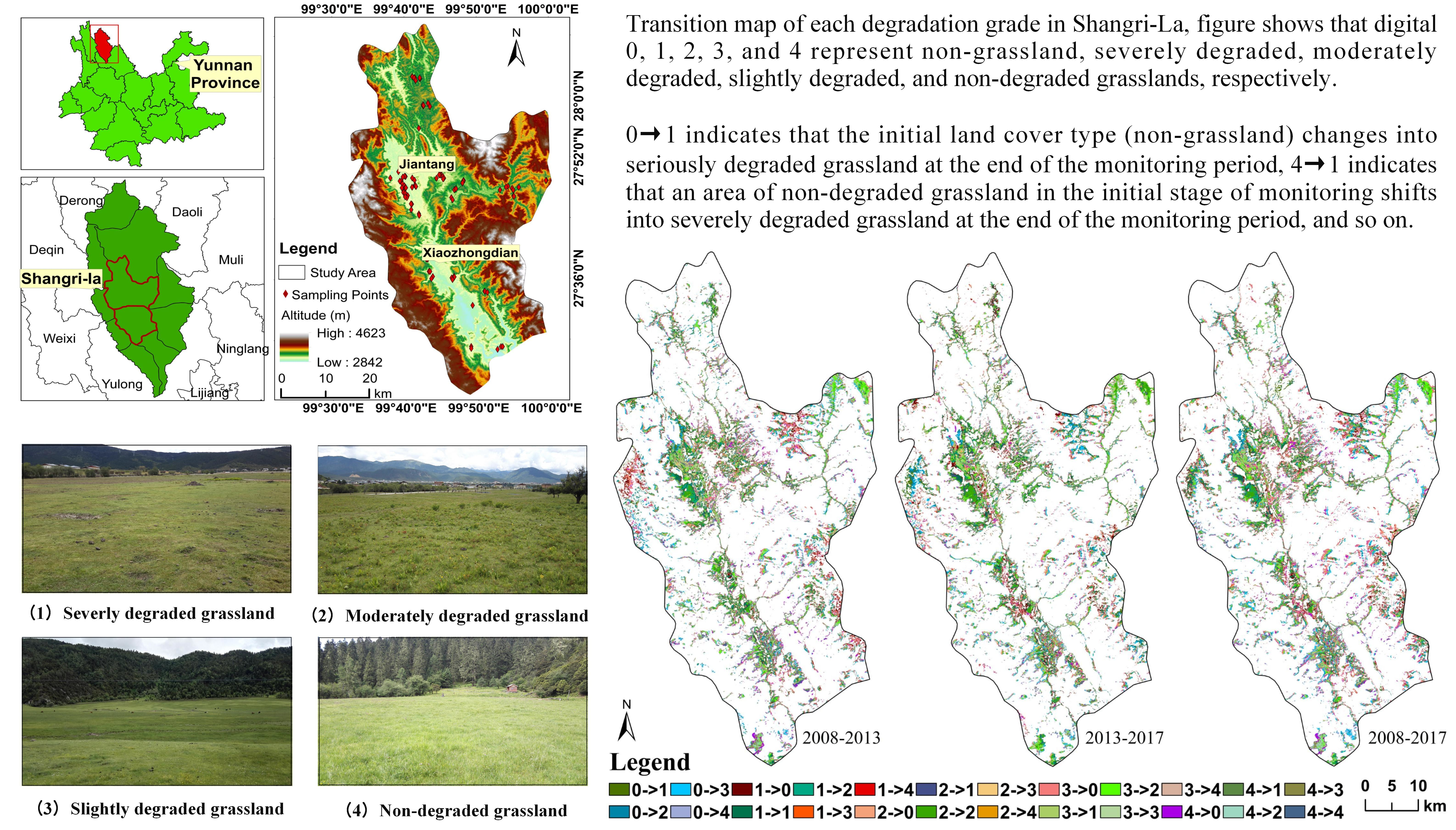
2.1. Study Area

Shangri-La is located in the eastern part of the Diqing Tibetan Autonomous Prefecture in northwestern Yunnan Province, China, and is in the hinterland of the world-famous natural heritage scenic site “Three Parallel Rivers”. In the centre of Shangri-La sit the towns of Jiantang and Xiaozhongdian, where the grasslands concentrate, with a longitude of 99°33′E–100°58’E and a latitude of 27°20′N–28°09’N, as shown in Figure 1.

The study area covers 2335.6 km², with an average elevation of 3450 m. With no summer season, the grasslands begin to turn green in May, wither at the end of October. The annual average temperature is 5.5 °C, and the annual average precipitation is 1100 mm. There are snow-capped mountains, deep valleys and vast grasslands. There are famous scenic spots such as the Dukezong Ancient City, the Pudacuo National Park, the Songzanlin Monastery, Napa Lake and Yila Grassland.

According to the natural conditions and use types of the study area, the grassland is divided into three categories: alpine meadow, subalpine (forest) meadow and swamp meadow, among which subalpine forest meadow is the most widely distributed and the largest in area. Surveys indicated that there are more than 106 grassland plants in the study area, including Leymus chinensis (Trin.) Tzvel, Poa annua L, Cyperus rotundus L, Carex spp., dandelion Taraxacum mongolicum (Hand.-Mazz), Potentilla fulgens Wall, Artemisia parviflora, Ligularia vellerea, Primula malacoides Franch, Erigeron breviscapus (Vant.) Hand.-Mazz, Euphorbia esula Linn, Euphorbia jolkinii, etc. [19]. The grassland type in Shangri-La is natural grassland. The local farmers raise livestock such as yak, horse, and Tibetan pig, most of which are grazed in free range instead of fixed ones. They hardly mow the grassland and feed the livestock with oat and highland barley stems in the winter.

2.2. Data Sources and Preprocessing

2.2.1. Huanjing 1 (HJ-1) Satellite Data

Remote-sensing data were obtained from China’s independent research and development Huanjing 1A and Huanjing 1B satellite (HJ-1A/B). Equipped with two charge coupled device (CCD) cameras of the same type, its footprint width is 700 km, and the ground pixel resolution is 30 m. Four wavebands are used: blue (wavelength range of 0.43–0.52 μm), green (wavelength range of 0.52–0.60 μm), red (wavelength range of 0.63–0.69 μm), and near-infrared (wavelength range of 0.76–0.90 μm). The study uses a total of 3 scene images. The satellite data on 9 October 2008, 10 October 2013 and 13 October 2017, adopted by this study are sourced from the China Centre for Resources Satellite Data and Application (http://www.cresda.com/CN/), and the original data have gone through basic preprocessing, including geometric correction, radiometric calibration and atmospheric correction on the ENVI 5.3 (Exelis Visual Information Solutions Inc., New York, NY, USA) platform.

2.2.2. Grassland Survey Data

The field investigation was conducted on 16 to 26 July and 24 September to 1 October in 2017 for a total of 17 days in the towns of Jiantang and Xiaozhongdian of Shangri-La covering 32 sample plots. With 3 quadrats for each plot, a total of 96 quadrats were investigated for data collection, including 49 in subalpine meadow, 18 in alpine meadow, and 29 in swamp meadow. This study used grasslands of consistent growing conditions with an area larger than 0.009 km² as samples. Each grassland sample point is placed over 100 m away from each other to ensure an effective and valid match between the sample points and the image pixel. With every sample points investigating 3 quadrat, each quadrat covers 1 m² and is 5 m apart from one another. The information for each quadrat about above-ground biomass, coverage, average height, number of species, edible herb biomass and inedible herb biomass was collected according to the standards in the Technical Regulation for Grassland Resource Survey (NY/T 2998-2016) [20], which is a standard issued by the Ministry of Agriculture of the People’s Republic of China.

2.3. Determination of the Grassland Degradation Evaluation System

2.3.1. Normalization of Evaluation Indicators

Among the grassland samples collected in the research field, the six indicators of aboveground biomass, average height, number of species, coverage, edible herb biomass and toxic weed biomass are indexes with different concepts of measurement units. In order to eliminate the impact of these different measurement units, normalization is required in processing each indicator to ensure that can quantitatively reflect the degradation of grassland. The normalization formula is shown in Equation (1).

$$x_i=\frac{X_i-X_{i\min }}{X_{i\max }+X_{i\min }}$$

(1)

where: x_i is the result of the normalization of i indicator; X_i is the original value of i indicator; X_imin is the minimum of i indicator; X_imax is the maximum value of i indicator.

2.3.2. Weight Calculation of Indicators

As the indicators of degraded grassland, such as coverage, average height, aboveground biomass and toxic weed biomass, differ from one another in their capability to indicate the degree of degradation, it is necessary to determine the weight of each indicator before calculating the GDI. Based on studies by Li [21] and Wu [22], factor analysis can be used to objectively and scientifically obtain the weights of each indicator. Factor analysis is an analysis method that evaluates abstract factors through specific indicators. This can transform multiple variables into few unrelated comprehensive indicators which can better reflect the characteristics and essence of things. Factor analysis can describe each variable of the original data by the sum of the linear function of the least number of common factor and the special factor. The variance contribution rate of the common factor can reflect its ability to interpret the total variance of the original variables. The higher the value becomes, the more important the factor is. The variance contribution rate of the common factor can be used to calculate the weight of the degraded grassland evaluation index. In this study, factor analysis method was carried out on six indicators to work out their weights in SPSS 22 (IBM SPSS Statistics Inc., New York, NY, USA) software.

2.3.3. Ground Comprehensive Evaluation Grassland Degradation Index (GDI_g) Calculation and Grading

The grassland GDI_g is a digital representation of the comprehensive evaluation of degraded grassland and a weighted summation of each degradation indicator. GDI_g value changes from 0 (most degraded) to 1 (less degraded). The survey found that the degraded grasslands in the study area had significant changes in the six indicators of above-ground biomass, average height, coverage, number of species, edible herb biomass and toxic weed biomass; therefore, these indicators were selected for grassland degradation evaluation. Moreover, the degraded grasslands in the research area experience toxic weed invasion. When calculating GDI_g, it is necessary to reduce the value of the toxic weed biomass to eliminate the phenomenon of GDI_g increasing instead of decreasing in response to toxic weed invasion. The formula for calculating GDI_g is shown in Equation (2):

$$GD{I}_{\mathrm{g}}={\displaystyle \sum _{i=1}^n{v}_i{w}_i-v_d{w}_d}$$

(2)

where GDI_g is the grassland ground evaluation index, n is the number of variables, v_i is the index normalization value, w_i is the indicator weight value, v_d is the toxic weed biomass normalization value, and w_d is the poisonous weed biomass weight value.

According to the GB 19377-2003 standard [18], the degrees of degraded grasslands in the study area are divided into four levels: non-degraded, mildly degraded, moderately degraded, and severely degraded. The calculated GDI_g values are arranged from small to large to indicate the degree of grassland degradation from strong to weak, which are ordered samples. Ordered sample optimal segmentation is the statistical method used for ordered samples and it can minimize the internal differences of each segment while maximizing external differences after segmentation [21]. It was used to determine the clustering statistics among the GDI_g values of degraded grasslands to carry out the division of each GDI_g indicating the degradation grade. The optimal segmentation of GDI_g is completed on the DPS7.5 (Data Processing System Hangzhou, Zhejiang, China,) software platform.

2.4. Construction of Remote-Sensing Models of Degraded Grasslands

The surface configuration of grasslands, such as biomass, coverage and other vegetation information, is closely related to the waveband information and vegetation index of remote-sensing image data [22,23]. The image waveband or vegetation index with the highest correlation with GDI_g, if known, can be used to construct a GDI_g and remote-sensing inversion model for the quantitative study of degraded grassland. Hence, this paper studies the correlation between the GDI_g and four HJ-I wavebands and the derived NDVI, renormalized difference vegetation index (RDVI), difference vegetation index (DVI), soil-adjusted vegetation index, (SAVI), perpendicular vegetation index (PVI), enhanced vegetation index, (EVI) and ratio vegetation index (RVI). The vegetation index calculation method is consistent with that of Yu [24], who found the remote-sensing data with the highest correlation for constructing the degraded grassland inversion model. The common vegetation index was extracted with HJ-1A/B satellite as the data source, and the correlation analysis with GDI was carried out to screen the most relevant remote-sensing vegetation index to construct the monitoring regression model.

Based on the GDIg value of the degraded grassland generated by the field survey in 2017, combined with the environment satellite-derived vegetation index RVI, the degraded grassland can be studied with high precision and quantification. Due to the inconsistent radiation conditions of environmental satellite images in different years, the radiation information detected cannot be evaluated by the same standard. To explore the degraded grassland in the study area in 2008 and 2013, it is necessary to perform radiation correction on the environmental image RVI of each year so that grassland degradation can be monitored by the same standard [15,25] RVI radiation registration is generally performed by establishing a radiation registration model for the ground objects that have not changed during the study period. The reason for this is that the radiation values obtained with the same type of sensor for the same ground object at different times should be equal or roughly equal.

The RVI₂₀₁₇ value derived from the environmental satellite data in 2017 was adopted as the standard with which to register the RVI₂₀₀₈ and RVI₂₀₁₃ values in the study area. In the images of three phases in 2008, 2013 and 2017, 480 points were discovered where no changes in ground objects occurred. After extracting the RVI₂₀₀₈, RVI₂₀₁₃, and RVI₂₀₁₇ values of these 480 points for a related analysis, a linear regression model for radiation correction is built to obtain the RVI radiation correction models.

2.5. Land-Use Classification Method in Research Area

In order to study the change of grassland distribution in Shangri-La in nearly 10 years from 2008 to 2017, the support vector machine (SVM) algorithm in the supervised classification is adopted, which has the characteristics of fast and high precision in the classification of features. According to the “Classification of Land Use Status” (GB/T 21010-2017) standard, the land use in the study area are classified into six first-grade types: farmland, forest, grassland, building land, water body, and ice and snow land. In the sample selection, since the separability of the ice and snow land and the bare land in the study area is less than 1, these two are combined into one type of ground object. With the ENVI5.3 platform referring to the historical images of Google Map in September 2017, the selection of local samples on environmental satellite images is carried out to ensure that the number of sample selections of each type is more than 400, and that the separability of each sample is larger than 1.9. In the meantime, with the 16-m resolution image of the GaoFeng 1 satellite of Jiantang Town in July 2017, after the geometric registration with the image of environmental satellite in 2017, 1000 points are generated randomly in the study area by using the random generation point function in the ArcGIS Map. The ground object type of the raster cell where each point is located is determined by manual visual interpretation as auxiliary data for verifying the accuracy of the classification result under the ENVI Post-Classification function.

2.6. Accuracy Test

2.6.1. GDI_g Evaluation Accuracy Test

The study selects the sample data collected from the south bank of Bitahai Nature Reserve as the indicator standard for non-degraded grassland. Based on the (GB 1977-2003) standard, 96 samples collected are classified by non-degraded grassland, slightly degraded grassland, moderately degraded grassland, and severely degraded grassland. The accuracy of degradation classification by GDI is tested by contrasting with the classification results based on GB (19377-2003) standard.

2.6.2. Fitting Model Accuracy Test

Over-fitting will occur in the process of establishing a grassland degradation monitoring model by linear fitting, and there will be some error in the inversion between the vegetation index and the ground-based degradation index. In order to test whether the model is applicable to the grassland degradation evaluation in the study area, it is necessary to carry out an accuracy test. The 30 verification group sample data collected at the same period were substituted into the fitted model to obtain the simulated GDI of the verification group, and then the relative error and root mean square error (RMSE) of the measured GDI values were calculated. The smaller the relative error is, the closer the result is to the real value. Relative error and RMSE calculation formulas are Formulas (3) and (4) respectively.

$$C=(GD{I}_g-GD{I}_{rs})/GD{I}_{\mathrm{g}}\times 100\%$$

(3)

$$RMSE=\sqrt{{\displaystyle {\sum }_{i=1}^n{(GD{I}_g-GD{I}_{\mathrm{r}s})}^2/n}}$$

(4)

where C is the relative error, RMSE is the root mean square error, and n is the number of samples, GDI_g is the ground observed value, and GDI_rs is the remote-sensing fitting value.

3. Results

3.1. GDI_g Calculation Results

The study carries out factor analysis on actual grassland measurement data within the SPSS 22 software to extract the variance of each indicator component. The cumulative variance contribution rate of the first two components reached 83.79%. With the rate of more than 80%, the grassland degradation information can use the first two principal components to replaces the original six evaluation indicators. Equations (5) and (6) show the linear combination equations of each index constructed according to the number of payloads and the eigenvalues of each indicator.

$$F_1=0.344x_1+0.509x_2+0.499x_3+0.187x_4+0.573x_5-0.104x_6$$

(5)

$$F_2=0.011x_1+0.196x_2+0.363x_3-0.620x_4+0.170x_5-0.645x_6$$

(6)

The variance contribution rates of these two principal components are taken as the weights of the grassland degradation indicators. Then the coefficients of the six indicators in the linear combination of the principal components are respectively weighted and averaged to obtain the comprehensive coefficient. Finally, the composite coefficients are normalized to obtain weight of indicator. The weights of the six indicators, including aboveground biomass, average height, coverage, number of species, biomass of edible herbs and biomass of toxic weeds, are 0.27, 0.12, 0.12, 0.14, 0.11 and 0.24, respectively.

By using Equation (2), the GDI_g values of 96 grassland quadrats were obtained to be between 0.165 and 0.782. In the DPS7.5 software, 96 sample data were segmented in an orderly manner. The four-segment segmentation results were used to represent the four levels of grassland degradation, and the GDI_g value corresponding to the dividing nodes is used as the threshold of each degradation level, as shown in

Table 1. GDI_g grading indicators for grassland degradation.

Degradation Level	Optimal Segmentation Result	GDIg Dividing Node
Non-degraded	92~96	GDIg ≥ 0.5162
Slight degradation	71~91	0.3757 ≤ GDIg < 0.5162
Moderate degradation	30~70	0.2560 ≤ GDIg < 0.3757
Severe degradation	1~29	GDIg < 0.2560

Note: The correspond GDI_g value of each interval is the demarcation standard of each degradation level, GDI_g is the grassland degradation index of ground comprehensive evaluation.

. The optimal classification result is the range of the partition interval, which is represented by ordinal classification in the ordered samples. Since the number of classifications is 4, samples numbered from 1–29 are grouped as one range, and samples 30–70, 71–91 and 92–96 are grouped as the other three ranges.

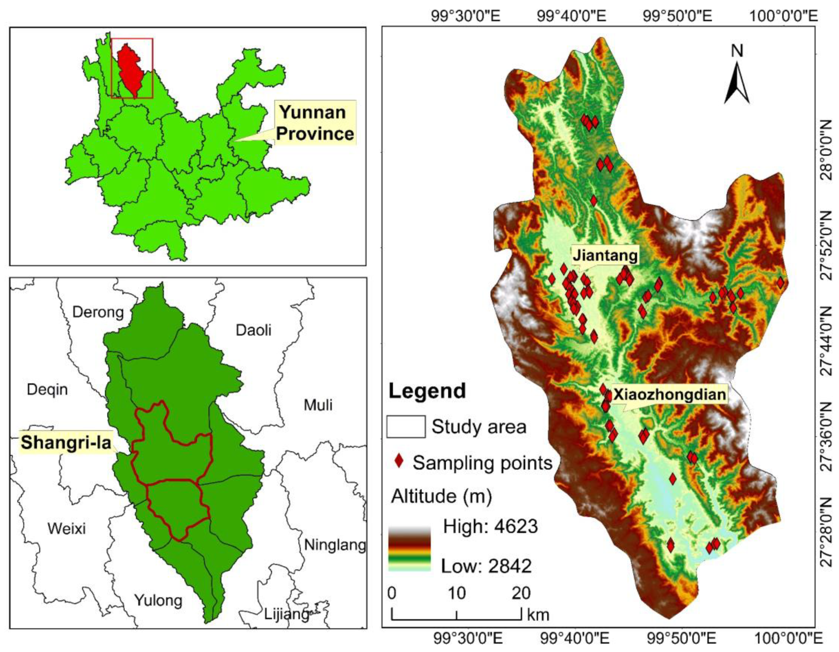
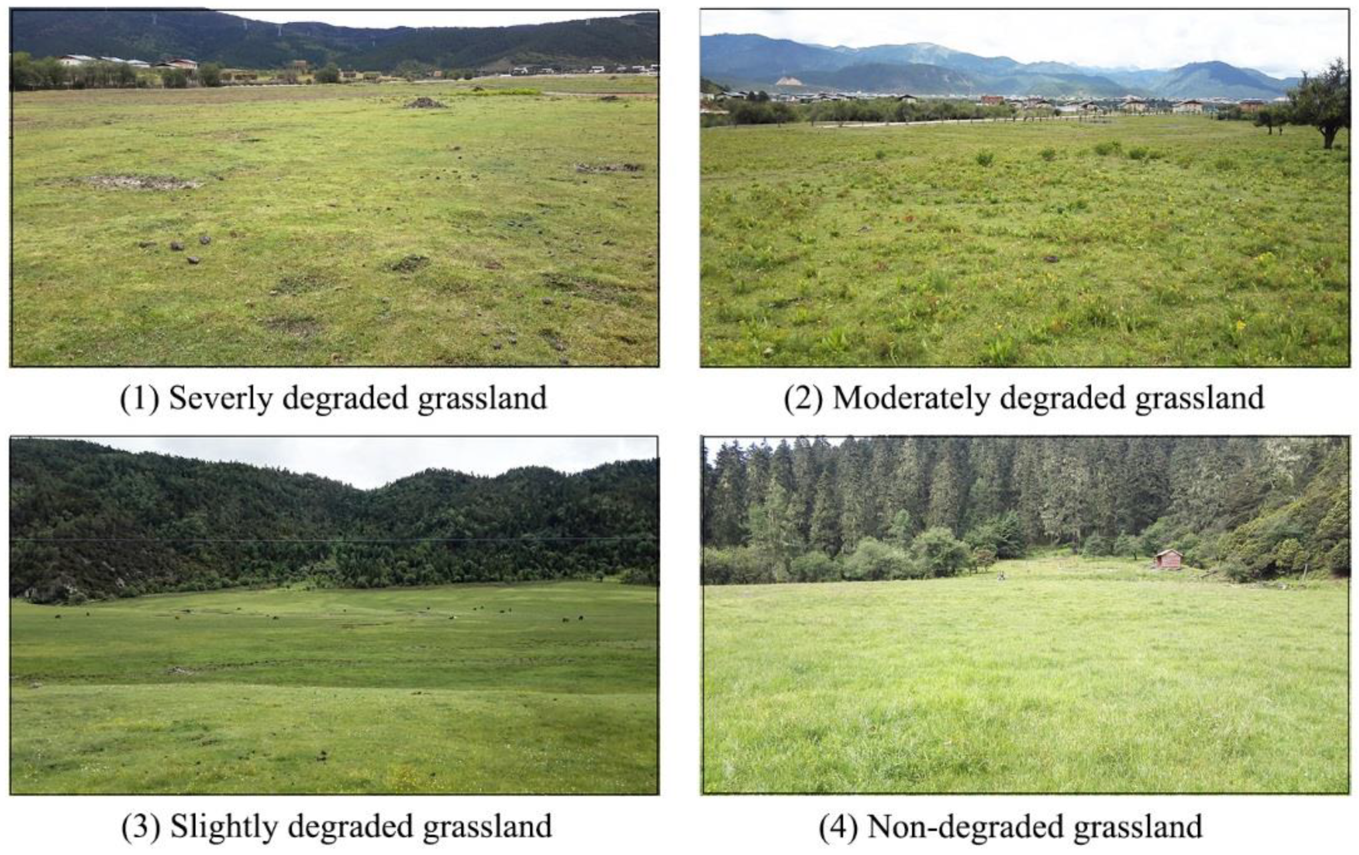
The non-degraded grassland is determined according to the GB 19377-2003 standard. The benchmark vegetation characteristics are based on the surface and soil conditions of the grasslands of the same use type in the demonstration zone near the monitoring site in natural grassland reserves with the same hydrothermal conditions. In line with the GB 19377-2003 standard, the 96 samples collected were evaluated for degradation grading, including 11 non-degraded, 15 mildly degraded, 42 moderately degraded and 28 severely degraded grassland samples. The accuracy of the GDI_g grading standard is verified in accordance with the GB 19377-2003 standard. Among them, 92 quadrats were consistent with the standard, with the grading accuracy reaching 95.83%. With such high accuracy, the GDI_g grading standards basically satisfy the grading of degraded grasslands. See

Table 2. Grassland quadrat survey results and grading standards.

Number	Above-Ground Biomass (g/m2)	Height (cm)	Coverage (%)	Number of Species	Edible Herb Biomass (g/m2)	Toxic Weed Biomass (g/m2)	GDIg Value	GDIg Graded Results	GB Graded Results
0	357	3	58	5	357	0	0.23	1	1
1	489	3	66	4	489	0	0.25	1	1
2	1630	20	100	8	1630	0	0.66	4	4
3	2152	22	100	8	2152	0	0.78	4	4
4	677	3	95	12	677	0	0.39	3	3
5	805	10	100	10	206	598	0.30	2	2
6	1203	12	100	11	1203	0	0.54	4	4
7	456	3	95	6	214	242	0.26	1	1
8	401	3	94	8	259	141	0.23	1	1
9	679	2	100	6	417	261	0.34	2	2
10	895	4	100	9	895	0	0.44	3	3
11	656	3	98	14	656	0	0.39	3	3
12	571	11	85	9	399	172	0.36	2	2

Note: Grassland biomass is fresh weight. Height is grass average height. Table 1, Table 2, Table 3 and Table 4 in the graded results represent severe degradation, moderate degradation, slight degradation and non-degraded grassland, respectively. GB is short for GB 19377-2003 standard.

for part of the quadrat survey data and grading standards. Degraded grassland grade landscape see Figure 2.

3.2. Remote-Sensing Models of Degraded Grasslands

The results of the correlation analysis of GDI_g with single HJ-1 wavebands and 7 common vegetation indexes analysed in this paper are presented in

Table 3. Correlation of GDI_g with single wavebands and 7 vegetation indexes.

Name	Correlation (R2)	Name	Correlation (R2)	Name	Correlation (R2)
b1	0.17	NDVI	0.69	PVI	0.61
b2	0.19	RDVI	0.39	EVI	0.38
b3	0.25	DVI	0.19	RVI	0.74
b4	0.02	SAVI	0.69	-	-

Note: b1, b2, b3 and b4 are the blue (0.43–0.52 μm), green (0.52–0.60 μm), red (0.63–0.69 μm) and the near-infrared (0.63–0.69 μm) wavebands, respectively. “-” represents a null value. NDVI is normalized difference vegetation index, RDVI is renormalized difference vegetation index, DVI is difference vegetation index, SAVI is soil-adjusted vegetation index, PVI is perpendicular vegetation index, EVI is enhanced vegetation index, and RVI is ratio vegetation index.

.

As shown in Table 3, the derived RVI of the environmental satellite image has the highest correlation with GDI_g. Hence, RVI and GDI_g are used to establish 11 regression models on the SPSS 22 platform with GDI_g as the dependent variable and RVI as the independent variable. Among the models, the power function regression model shows the optimal fitting (R² is 0.765). The established grassland degradation evaluation index of remote-sensing GDI_rs inversion is shown in Equation (7).

$$GD{I}_{rs}=0.076\times RV{I}_{2017}^1.15$$

(7)

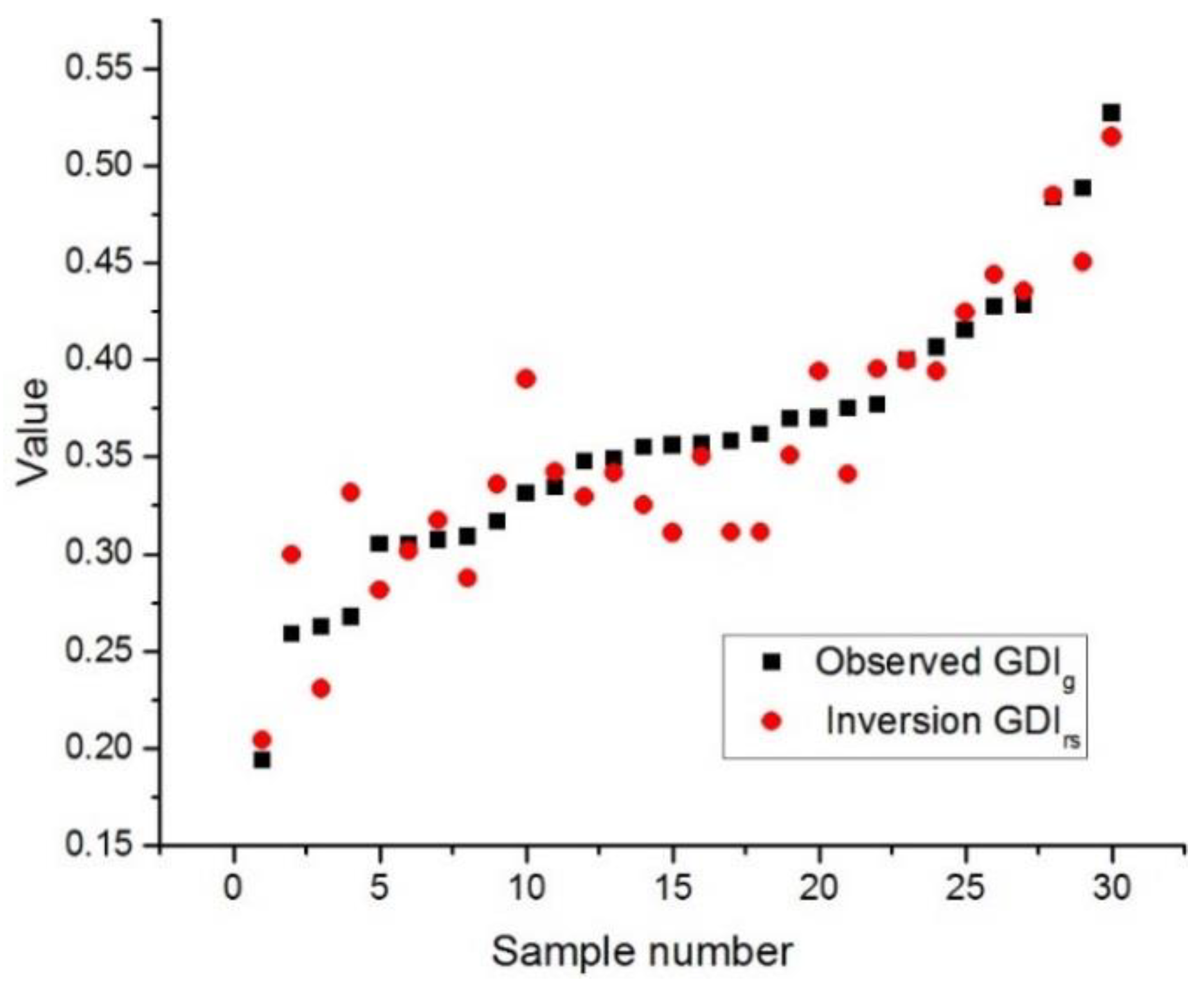
To test the accuracy of the fitting values of the constructed GDI_rs regression models, 30 grassland quadrats are selected as experimental groups, as shown in Figure 3. The relative error of the comparison of the GDI_rs of RVI with the real GDI_g is 3.61%, and RMSE value is 0.736.

The RVI₂₀₀₈, RVI₂₀₁₃, and RVI₂₀₁₇ correction models are as shown in Equations (8) and (9).

$$RV{I}_{2017}=0.608RV{I}_{2008}+1.422$$

(8)

$$RV{I}_{2017}=0.884RV{I}_{2013}+0.253$$

(9)

where RVI₂₀₁₇ is the value of RVI in the year 2017, RVI₂₀₁₃ is the value of RVI in the year 2013, RVI₂₀₀₈ is the value of RVI in the year 2008.

The grassland area, grassland degradation status and transformation of degraded grassland in the study area in 2008, 2013 and 2017 are obtained based on the established degraded grassland GDI_rs inversion model along with the grassland degradation evaluation system (Table 1) and the statistical analysis of remote-sensing data and geographic information.

3.3. Change in Grassland Area

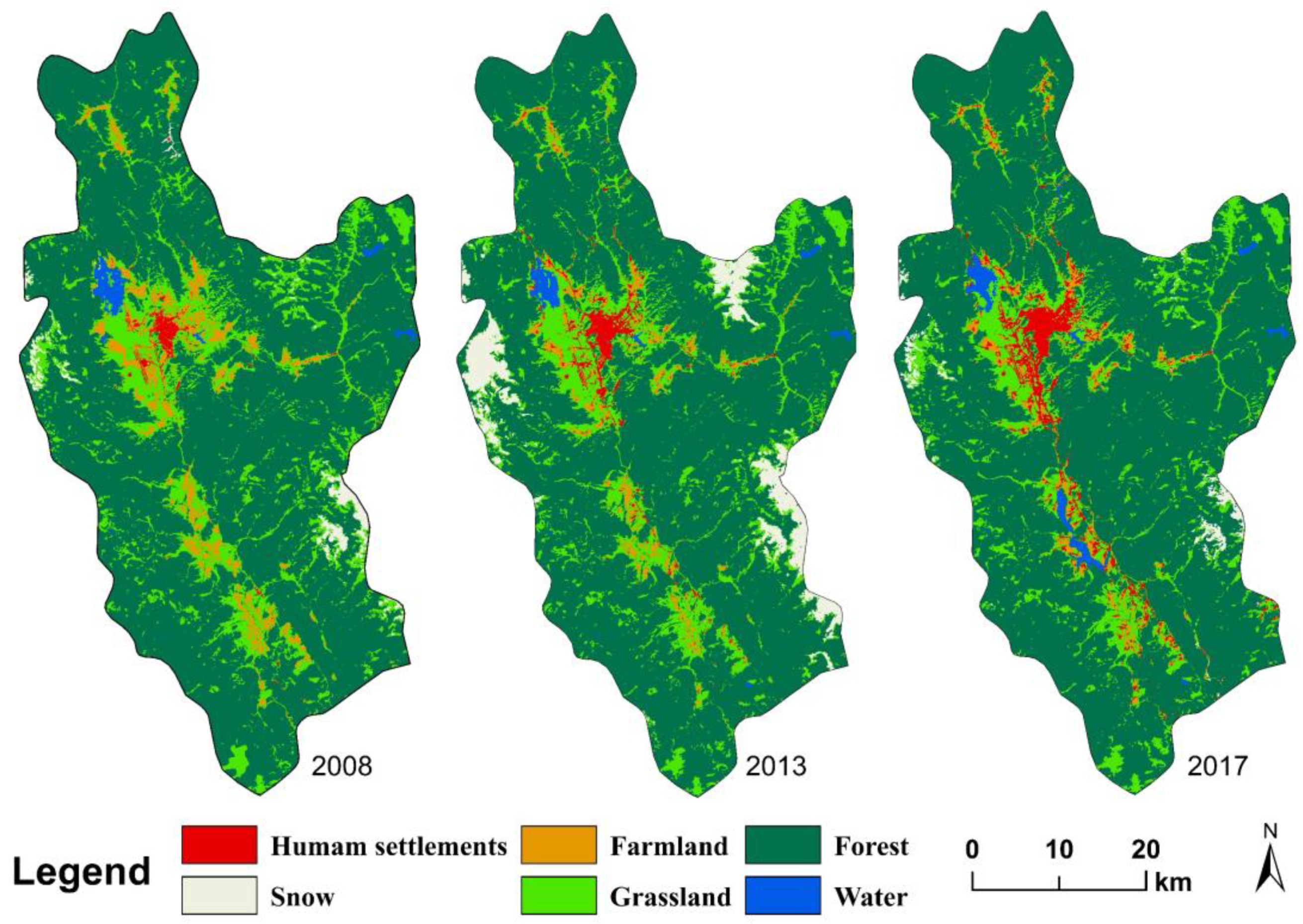
In the past 10 years, land-use has undergone significant changes in the study area [26]. The overall classification accuracy is 85.6%. The land-use classification results are shown in Figure 4.

The land-use results for each year in the study area are obtained by the statistical analysis of geographic information, as shown in

Table 4. Statistical table of land-use areas by year.

Year	Type	Forest	Farmland	Grassland	Water Body	Human Settlement	Snow
2008	Area (km2)	1789.82	71.24	405.40	18.28	18.85	32.14
	Ratio (%)	76.82	3.02	17.26	0.80	0.78	1.36
2013	Area (km2)	1802.43	51.72	378.29	16.94	41.88	64.47
	Ratio (%)	76.53	2.20	16.06	0.72	1.78	2.74
2017	Area (km2)	1845.70	47.28	338.87	25.62	74.80	23.45
	Ratio (%)	78.35	2.01	14.39	1.09	3.18	1.00

. In the study area, forest was the most widely distributed land-use type, accounting for 76.82% of the total area in 2008. It dominated in the area above 3700 m, where it encircled the lower region, and underwent little change in the last decade. Total farmland, just a small area mainly in the towns of Jiantang and Xiaozhongdian, accounted for 3.02% of the total area in 2008, and decreased from 71.24 km² to 47.28 km² from 2008 to 2017.

Ranked second, grassland, which was concentrated in the centre of the study area and inter-mountain valley areas, accounts for 17.26% of the total area in 2008. From 2008 to 2017, the grassland area decreased by 66.53 km² at a rate of approximately 1.82% per year. It was primarily converted into farmland and human settlements land, which was concentrated in the centre district of the town of Jiantang. The decrease in grassland has a direct impact on the total growth of the grassland, thus increasing the livestock grazing pressure at the same grazing level. Human settlements accounting for 0.78% of the total area in 2008 experienced rapid growth from 18.85 km² to 74.80 km² from 2008 to 2017. The water body area, accounting for 0.80% of the total area, was mainly composed of Napa Lake, Bita Lake and Shudu Lake. In August 2014, the Xiaozhongdian reservoir was completed, and the water body area of the research area increased to 25.62 km² in 2017. Snow land, making up 1.36% of the total area in 2008, was distributed in areas with an altitude of more than 4000 m and was concentrated in the west and southeast of the research area. As snow fell in Shangri-La earlier than usual in 2013, some areas in the research area were covered by snow and ice, the area of snow and ice covered land increased to 64.47 km² in 2013.

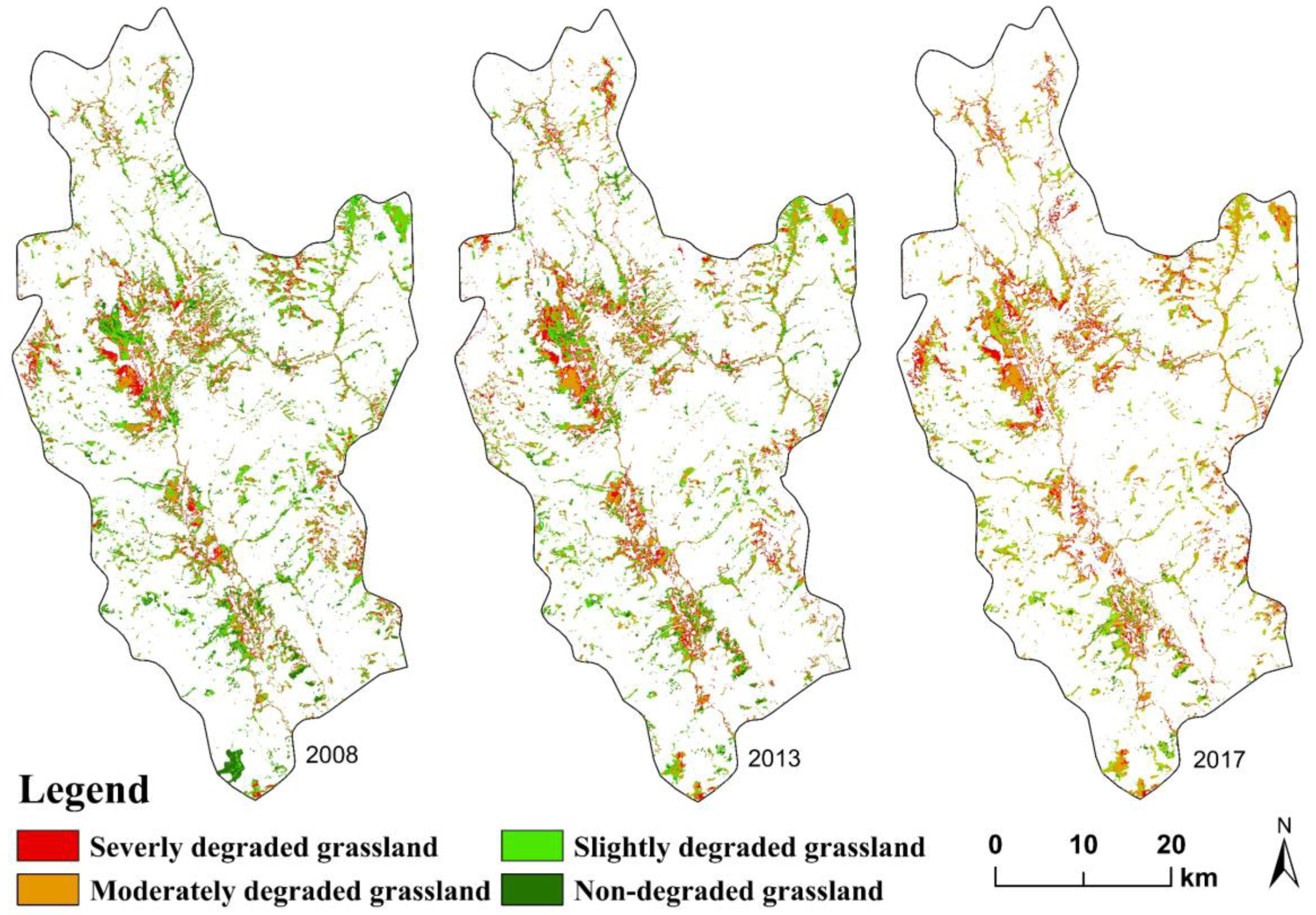
3.4. Distribution Status of Degraded Grassland

Remote-sensing identification was carried out to identify the severely degraded, moderately degraded, slightly degraded and non-degraded regions in the study area in 2008, 2013 and 2017 based on the constructed degraded grassland inversion Equation (2) and the established grassland degradation grading standard in the ENVI5.3 platform. The results are shown in Figure 5.

As shown in Figure 5, the grassland was scattered throughout the study area, with clusters gathering in the centre and strips expanding outwards. This pattern was formed by complex and diverse topographic features such as alpine flats and terraces. On the whole, the grasslands degraded from the centre to the edge, and the degradation intensity presented a strong–weak–strong spatial distribution. The non-degraded grassland was mainly around Napa Lake, Bita Lake Nature Reserve and the mountain valley area at the centre of the study area, where there were thick soil layers, flat terrain, abundant water and heat, and excellent natural conditions for grassland growth. The slightly degraded grassland, which shared a similar distribution with that of the moderately degraded grassland, was sparsely distributed around the severely degraded grassland. The moderately degraded grassland was distributed in strips from north to south, close to the centre of the towns of Jiantang and Xiaozhongdian. The severely degraded grassland was concentrated on the mountain peaks above 4000 m and on the western side of the town of Jiantang. The areas high in the mountains, where grasslands were severely degraded, have to withstand a thin soil layer, the frequent occurrence of extreme weather, and poor conditions for grass growth. This was the main factor leading to the degradation of alpine grassland. Species such as Stellera chamaejasme L. and Euphorbia nematocypha Hand-Mazz are highly invasive in the grassland on the western side of the town of Jiantang so there are few edible herbs. The RVI value of this area was low in October as the toxic weed clusters began to wither and turn yellow.

The non-degraded grassland showed a significant change, decreasing by 59.87 km² in 10 years, and the slightly degraded grassland also showed a downward trend, decreasing by 49.93 km² from 2008 to 2017, with a fast rate of decrease. The moderately degraded grassland accounted for 39.17% of the grassland area in 2017 and grew by 41.17 km² from 2008 to 2017. The area of severely degraded grassland accounting for 23.11% of the total area in 2017, changed little, fluctuating in the range from 77 to 87 km². See

Table 5. Grassland area and proportion of each degradation grade in 2008, 2013 and 2017.

Degree of Degradation	2008		2013		2017
	Area (km2)	Proportion (%)	Area (km2)	Proportion (%)	Area (km2)	Proportion (%)
Non-degraded	85.68	21.14	51.21	13.54	25.81	7.62
Slight	150.92	37.23	115.34	30.49	101.99	30.10
Moderate	91.58	22.58	124.36	32.87	132.74	39.17
Severe	77.21	19.05	87.38	23.10	78.32	23.11
Grassland area	405.40	100.00	378.29	100.00	338.87	100.00

for the statistics of the grassland area of each degraded grade in 2008, 2013 and 2017.

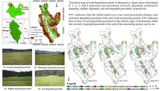
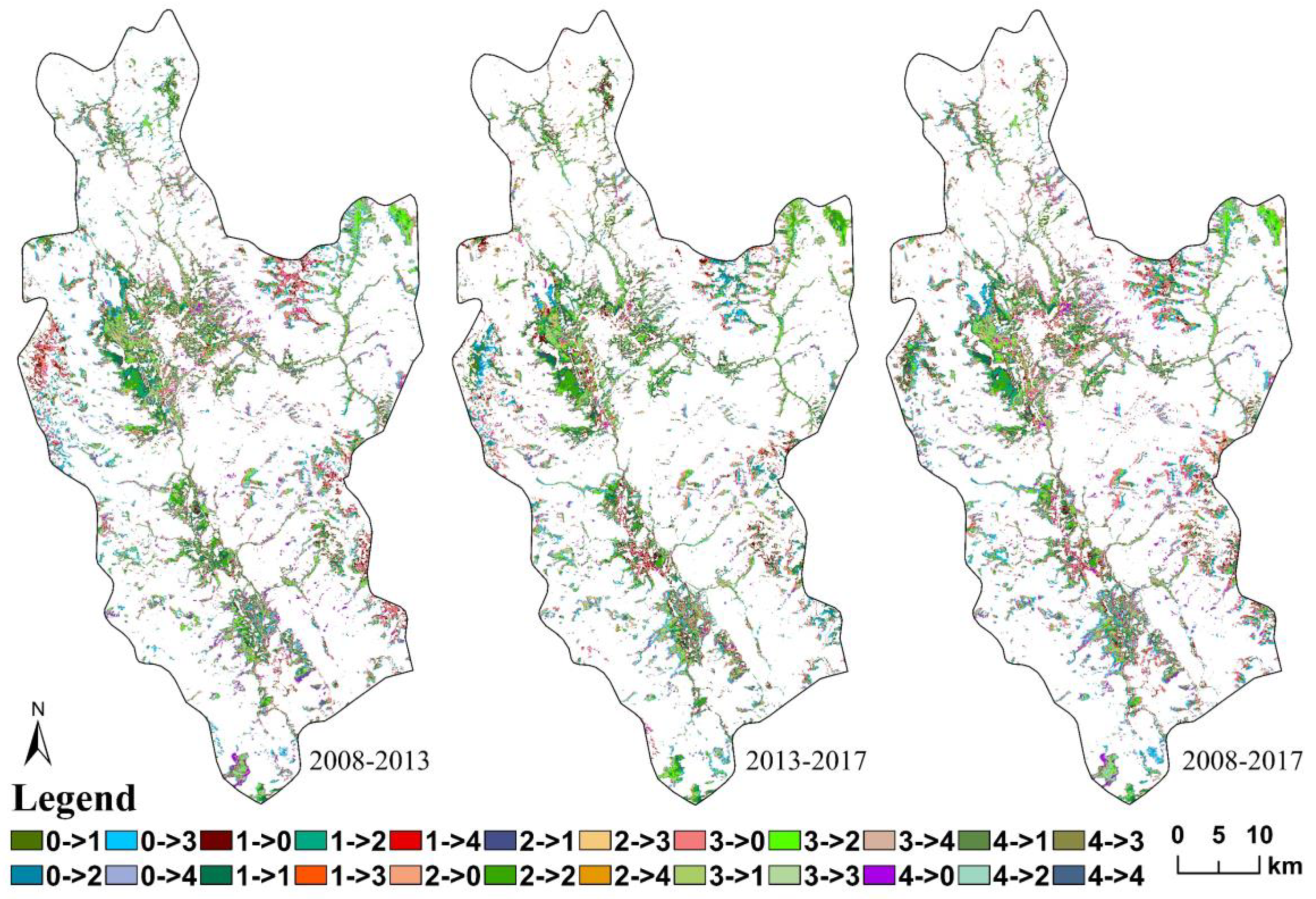
3.5. Dynamic Change in the Degraded Grassland

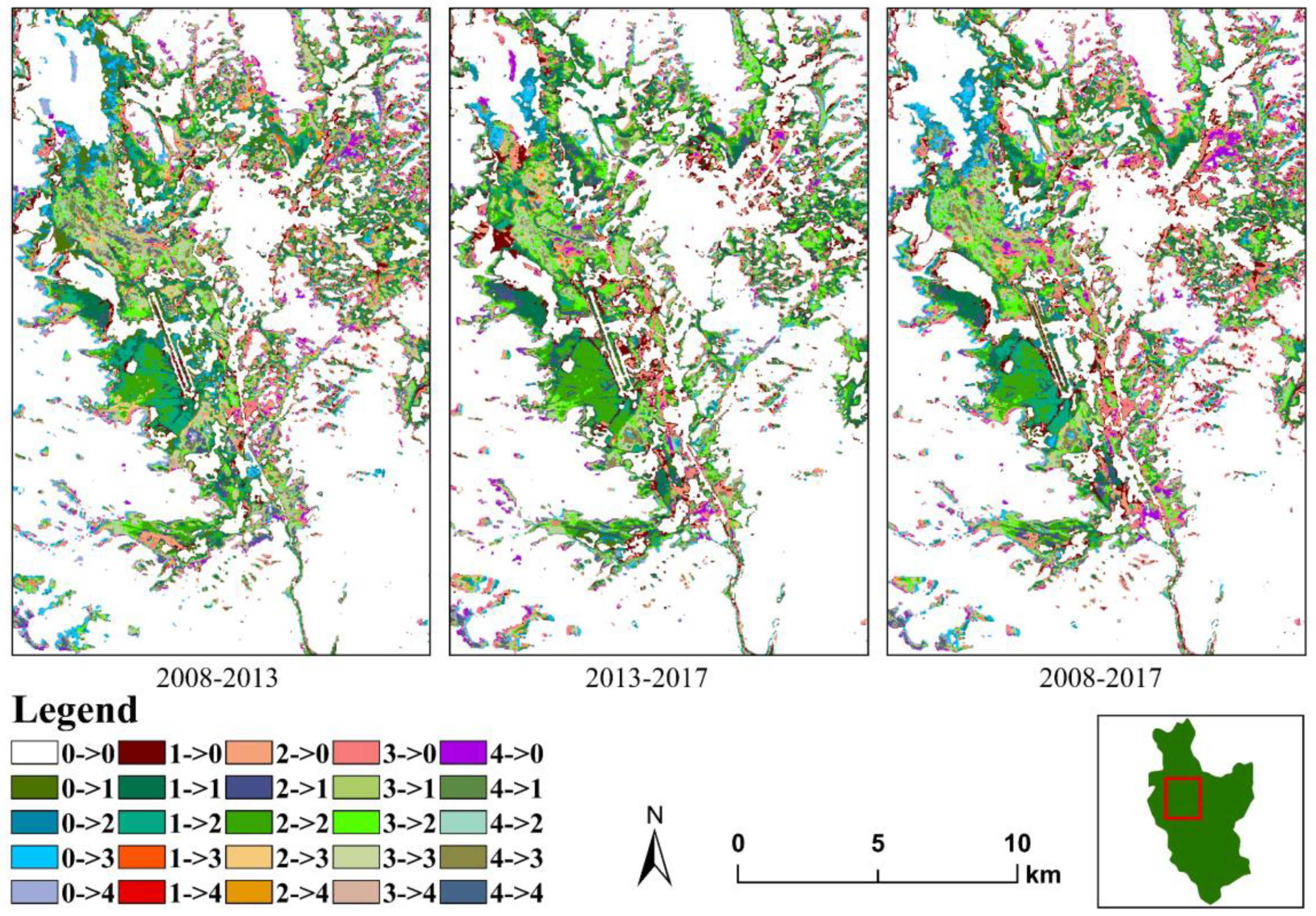
To analyse the dynamic process of degraded grasslands in an in-depth manner and grasp the characteristics of the dynamic evolution among the various degradation grades, the spatial transformation analysis of each degradation grade in 2008, 2013 and 2017 was conducted in the ArcGIS 10.2 platform. As shown in Figure 6 and Figure 7.

In Figure 6 it is shown that the degradation grades of the study area are dominated by small, scattered patches, concentrated near the central part of the town of Jiantang. In addition, the grasslands near the western, northeastern and southeastern borders of the study area changed significantly, while the large patches in the western area near the Diqing Airport, Bita Lake Reserve, Napa Lake and Yila Grassland remained relatively stable in degradation grade. In the periods of 2008–2013, 2013–2017, and 2008–2017, there were 240.10 km², 238.57 km², and 195.95 km², respectively, that did not undergo grade shifting. The majority of the grassland did not change, and the grassland grade change showed a flat increase. In the three periods, the areas of grasslands that underwent a degradation grade change were 165.29 km², 139.72 km², and 209.45 km², respectively, and the area of changed grassland increased gradually.

From the perspective of grassland ecology, degradation grade transitioning from slight to moderate or severe is called grassland degradation aggravation (deterioration) and indicates negative succession, while transitioning from moderate or severe to slight or non-degradation is called degradation restoration and indicates positive succession [20]. According to the statistics, the areas of aggravated grassland in 2008–2013, 2013–2017, and 2008–2017 were 99.89 km², 58.41 km², and 111.50 km², respectively; those of restored grassland in each period were 37.82 km², 39.71 km², and 30.37 km², respectively. The total restored area is small and is far less than that of the aggravated area. As the degradation is dominated by aggravation on the whole, the degradation situation cannot be seen as optimistic. See

Table 6. 2008–2013 grassland degradation grade transfer matrix.

2008	2013
	Non (km2)	Slightly (km2)	Moderately (km2)	Severely (km2)	Non-Grass (km2)
Non	42.00	20.54	10.11	5.50	7.53
Slightly	5.26	81.59	32.41	16.42	15.25
Moderately	2.71	7.17	65.25	14.91	1.14
Severely	1.14	5.67	15.88	51.26	3.28
Non-grass	0.10	0.37	0.71	0.30	1949.32

,

Table 7. 2013–2017 grassland degradation grade transfer matrix.

2013	2017
	Non (km2)	Slightly (km2)	Moderately (km2)	Severely (km2)	Non-Grass (km2)
Non	18.78	16.40	6.35	1.85	7.83
Slightly	4.73	67.62	18.85	4.33	19.80
Moderately	1.48	14.15	91.04	10.62	7.07
Severely	0.51	3.56	15.27	61.13	4.91
Non-grass	0.31	0.26	1.23	0.39	1975.23

and

Table 8. 2008–2017 grassland degradation grade transfer matrix.

2008	2017
	Non (km2)	Slightly (km2)	Moderately (km2)	Severely (km2)	Non-Grass (km2)
Non	18.61	28.33	22.32	4.16	12.22
Slightly	4.45	63.06	33.15	11.02	39.24
Moderately	1.34	7.22	62.35	12.51	8.15
Severely	0.70	2.30	14.36	51.94	6.91
Non-grass	0.72	1.09	0.55	0.68	1947.32

for details of the degradation grades.

4. Discussion

4.1. GDI_g Theory and Accuracy

In past grassland degradation monitoring, grassland coverage and biomass were used as indicators of whether grassland degradation occurred, and other indicators of grassland vegetation were paid no attention to. Under the unfavourable influence of natural conditions of soil, rainfall, climate that are not conducive to the vegetation growth and of human factors such as overgrazing, adverse change would take place in the height of vegetation, coverage, edible herb ratio, etc. Therefore, this is not a comprehensive way to use a single indicator of coverage or biomass to assess grassland degradation. The GDI index, integrating aboveground biomass, average height, coverage, number of species, edible herb biomass and toxic weed biomass, can determine if the degradation occurs from two aspects-the health of grassland vegetation itself and availability for human use. These six indicators can accurately detect the changes of grassland, making the grading on degraded grassland more precise that can reach as high as 95.8%. Compared with GDI based on three degradation indicators of Du [15], Feng [27] and Li [14], the evaluation accuracy is largely improved.

Based on ETM+ image, Li [25] calculated the degraded grassland coverage in Yanchi County, Ningxia Province, China, to monitor grassland variation, with an assessed grassland degradation accuracy of 80%; based on Landsat TM/ETM image; Li [28] used mixed classification method to identify the degraded grassland in the central region of Northern Tibet, with an accuracy of 78%. Compared with coverage and mixed classification method, GDI-based evaluation is of higher accuracy in grading grassland degradation. Moreover, the flexible selection of GDI indicators is mainly determined by the indicators of vegetation changes in the study area when the vegetation degrades. The more specific the indicators, the stronger the ability to indicate degradation. However, being too much specific is not necessarily better.

4.2. Applicability of GDI

GDI requires non-degraded grassland as the reference so as to determine whether grassland degradation occurs, thus the selection of non-degraded grassland type becomes very important. With soil properties and climate type varying in different areas, there are diversified types of grassland with various grassland vegetation communities under natural conditions. For example, the alpine meadow type, whose average vegetation height and species number are significantly different from that of tropical grass. It is obviously unscientific to select the non-degraded grassland of the tropical grass as a reference to determine the degradation of the alpine meadow. Generally, the grassland that has not been affected by human activities in the local nature reserve is used as a reference object, which also limits the use of GDI for degraded grassland assessment in a large area. For this reason, when monitoring degraded grassland with GDI, selected samples of non-degraded grassland should be suitable for the whole area. GDI-based grassland degradation monitoring is applicable to small areas (counties, prefectures) where grassland degradation can be identified with high precision.

It is noteworthy that GDI can sensitively capture the changes of grassland vegetation, the grassland that early growth stage and mowed by herdsmen stage cannot be used as samples, these stage grassland will be evaluated as severely degraded grassland. When using GDI to monitor grassland degradation, maturation grassland must be selected.

4.3. Grassland Degradation Characteristics and Impact Factors

From 2008 to 2017, the grassland area in the study area decreased by 66.53 km², the loss of which was mainly concentrated in the vicinity of urban areas of Jiantang Town and Xiaozhongdian Town; the construction land increased by 55.95 km² within 10 years. In terms of land conversion, the lost grassland was mainly converted into construction land, which is consistent with the research results of Ma [26] and Lu [29]. The urban area near Jiantang town is endowed with favourable growth conditions such as fertile soil and abundant water and heat. Why is the severely degraded grassland widely distributed in this area? Wu [30] suggests in his research that the main reason for grassland degradation in Shangri-La is overgrazing. The herdsmen are concentrated in the urban area of Jiantang Town and they raise livestock nearby, leading to severe grassland degradation in the area. Non-degraded and slightly degraded grasslands are distributed intensively around the Napa Sea. The grassland around Napahai wetland grow well under the same artificial conditions, as in only 4 out of the 29 wetlands investigated degradation occured. The marsh grassland contains a larger volume of water, which provides stable water for grassland growth, indicating that the marsh grassland has stronger anti-degradation ability.

From 2008 to 2017, the grassland in the whole region was in continuous degradation, with the area of moderately degraded grassland increasing by 41.17 km²; the number of livestock in Shangri-La increased by 94,900 from 570,700 to 564,600. The grassland degradation in the study area was mainly the result of overgrazing. The field investigation finds that the local Tibetan pigs that are generally free range like to eat leaf stalks and roots, leaving large grasslands eaten in the Yila grassland and other areas, where vegetation is almost ruined. Famous for its beautiful scenery, Shangri-La attracts a large number of tourists, most of whom come to walk, rest, camp and barbecue on the grassland, trampling on the grassland, throwing away garbage and pouring soda at will, all of which cause different degrees of damage to the grassland. Moreover, Wu [30] thinks that the main reasons for grassland degradation also includes unimproved grazing regulations, overgrazing, farmers’ closed operation mode, and single production structure. To improve this, the local government should make reasonable plans on city construction, introduce scientific zoning management, increase the artificial grassland, and strengthen the grassland protection education.

5. Conclusions

This study explores the feasibility of using GDI in remote-sensing monitoring of degraded grasslands. From the maps and data obtained, the GDI_g, constructed on the basis of aboveground biomass, average height, coverage, number of species, biomass of edible herb, biomass of toxic weeds, can quantitatively indicate the degradation status of grassland, and the accuracy of grassland degradation classification with GDI value reaches 95.83%. Compared with indicators of coverage and biomass, GDI is a more comprehensive and effective method to evaluate whether grassland degradation happens. But different types of grassland in the study area should be taken into consideration when monitoring degraded grassland with GDI, because big differences in grassland types may affect the GDI evaluation accuracy. It is of great value to continue exploring the GDI application in remote-sensing monitoring of grassland degradation. In the future research, we should study the degradation resistance of different grassland types and the accuracy of GDI in degradation evaluation of different grassland types.

In the study, a remote-sensing model based on GDI was used to monitor grassland degradation in Shangri-La from 2008 to 2017. The main degradation of grassland was marked by the significant reduction of grassland area, decreasing by 66.53 km² during the monitoring period. In addition, there were evident changes in the degradation grade, from non-degradation and slight degradation to moderate degradation. The area of moderately degraded grassland increased from 22.58% in 2008 to 39.17% in 2017, deteriorating year by year. As grassland degradation was mainly caused by excessive livestock raising and extensive management of local herdsmen, the government in the future should limit the amount of livestock, increase the area of artificial grassland, and control the loss of grassland, so as to ensure the healthy development of grassland ecology in Shangri-La.